
|
|
|
 View source on GitHub View source on GitHub
|
|
To do machine learning in TensorFlow, you are likely to need to define, save, and restore a model.
A model is, abstractly:
- A function that computes something on tensors (a forward pass)
- Some variables that can be updated in response to training
In this guide, you will go below the surface of Keras to see how TensorFlow models are defined. This looks at how TensorFlow collects variables and models, as well as how they are saved and restored.
Setup
import tensorflow as tf
import keras
from datetime import datetime

%load_ext tensorboard
2023-10-18 01:21:05.536666: E tensorflow/compiler/xla/stream_executor/cuda/cuda_dnn.cc:9342] Unable to register cuDNN factory: Attempting to register factory for plugin cuDNN when one has already been registered
2023-10-18 01:21:05.536712: E tensorflow/compiler/xla/stream_executor/cuda/cuda_fft.cc:609] Unable to register cuFFT factory: Attempting to register factory for plugin cuFFT when one has already been registered
2023-10-18 01:21:05.536766: E tensorflow/compiler/xla/stream_executor/cuda/cuda_blas.cc:1518] Unable to register cuBLAS factory: Attempting to register factory for plugin cuBLAS when one has already been registered
TensorFlow Modules
Most models are made of layers. Layers are functions with a known mathematical structure that can be reused and have trainable variables. In TensorFlow, most high-level implementations of layers and models, such as Keras or Sonnet, are built on the same foundational class: tf.Module.
Building Modules
Here's an example of a very simple tf.Module that operates on a scalar tensor:
class SimpleModule(tf.Module):
  def __init__(self, name=None):
    super().__init__(name=name)
    self.a_variable = tf.Variable(5.0, name="train_me")
    self.non_trainable_variable = tf.Variable(5.0, trainable=False, name="do_not_train_me")
  def __call__(self, x):
    return self.a_variable * x + self.non_trainable_variable

simple_module = SimpleModule(name="simple")

simple_module(tf.constant(5.0))
2023-10-18 01:21:08.181350: W tensorflow/core/common_runtime/gpu/gpu_device.cc:2211] Cannot dlopen some GPU libraries. Please make sure the missing libraries mentioned above are installed properly if you would like to use GPU. Follow the guide at https://www.tensorflow.org/install/gpu for how to download and setup the required libraries for your platform.
Skipping registering GPU devices...
<tf.Tensor: shape=(), dtype=float32, numpy=30.0>
Modules and, by extension, layers are deep-learning terminology for "objects": they have internal state, and methods that use that state.
There is nothing special about __call__ except to act like a Python callable; you can invoke your models with whatever functions you wish.
You can set the trainability of variables on and off for any reason, including freezing layers and variables during fine-tuning.
By subclassing tf.Module, any tf.Variable or tf.Module instances assigned to this object's properties are automatically collected. This allows you to save and load variables, and also create collections of tf.Modules.
# All trainable variables
print("trainable variables:", simple_module.trainable_variables)
# Every variable
print("all variables:", simple_module.variables)
trainable variables: (<tf.Variable 'train_me:0' shape=() dtype=float32, numpy=5.0>,)
all variables: (<tf.Variable 'train_me:0' shape=() dtype=float32, numpy=5.0>, <tf.Variable 'do_not_train_me:0' shape=() dtype=float32, numpy=5.0>)
This is an example of a two-layer linear layer model made out of modules.
First a dense (linear) layer:
class Dense(tf.Module):
  def __init__(self, in_features, out_features, name=None):
    super().__init__(name=name)
    self.w = tf.Variable(
      tf.random.normal([in_features, out_features]), name='w')
    self.b = tf.Variable(tf.zeros([out_features]), name='b')
  def __call__(self, x):
    y = tf.matmul(x, self.w) + self.b
    return tf.nn.relu(y)
And then the complete model, which makes two layer instances and applies them:
class SequentialModule(tf.Module):
  def __init__(self, name=None):
    super().__init__(name=name)

    self.dense_1 = Dense(in_features=3, out_features=3)
    self.dense_2 = Dense(in_features=3, out_features=2)

  def __call__(self, x):
    x = self.dense_1(x)
    return self.dense_2(x)

# You have made a model!
my_model = SequentialModule(name="the_model")

# Call it, with random results
print("Model results:", my_model(tf.constant([[2.0, 2.0, 2.0]])))
Model results: tf.Tensor([[0. 3.415034]], shape=(1, 2), dtype=float32)
tf.Module instances will automatically collect, recursively, any tf.Variable or tf.Module instances assigned to it. This allows you to manage collections of tf.Modules with a single model instance, and save and load whole models.
print("Submodules:", my_model.submodules)
Submodules: (<__main__.Dense object at 0x7f7931aea250>, <__main__.Dense object at 0x7f77ed5b8a00>)
for var in my_model.variables:
  print(var, "\n")
<tf.Variable 'b:0' shape=(3,) dtype=float32, numpy=array([0., 0., 0.], dtype=float32)>

<tf.Variable 'w:0' shape=(3, 3) dtype=float32, numpy=
array([[-2.8161757, -2.6065955,  1.9061812],
       [-0.9430401, -0.4624743, -0.4531979],
       [-1.3428234,  0.7062293,  0.7874674]], dtype=float32)>

<tf.Variable 'b:0' shape=(2,) dtype=float32, numpy=array([0., 0.], dtype=float32)>

<tf.Variable 'w:0' shape=(3, 2) dtype=float32, numpy=
array([[ 1.0474309 , -0.6920227 ],
       [ 1.2405277 ,  0.36411622],
       [-1.6990206 ,  0.762131  ]], dtype=float32)>
Waiting to create variables
You may have noticed here that you have to define both input and output sizes to the layer. This is so the w variable has a known shape and can be allocated.
By deferring variable creation to the first time the module is called with a specific input shape, you do not need specify the input size up front.
class FlexibleDenseModule(tf.Module):
  # Note: No need for `in_features`
  def __init__(self, out_features, name=None):
    super().__init__(name=name)
    self.is_built = False
    self.out_features = out_features

  def __call__(self, x):
    # Create variables on first call.
    if not self.is_built:
      self.w = tf.Variable(
        tf.random.normal([x.shape[-1], self.out_features]), name='w')
      self.b = tf.Variable(tf.zeros([self.out_features]), name='b')
      self.is_built = True

    y = tf.matmul(x, self.w) + self.b
    return tf.nn.relu(y)
# Used in a module
class MySequentialModule(tf.Module):
  def __init__(self, name=None):
    super().__init__(name=name)

    self.dense_1 = FlexibleDenseModule(out_features=3)
    self.dense_2 = FlexibleDenseModule(out_features=2)

  def __call__(self, x):
    x = self.dense_1(x)
    return self.dense_2(x)

my_model = MySequentialModule(name="the_model")
print("Model results:", my_model(tf.constant([[2.0, 2.0, 2.0]])))
Model results: tf.Tensor([[0. 0.]], shape=(1, 2), dtype=float32)
This flexibility is why TensorFlow layers often only need to specify the shape of their outputs, such as in tf.keras.layers.Dense, rather than both the input and output size.
Saving weights
You can save a tf.Module as both a checkpoint and a SavedModel.
Checkpoints are just the weights (that is, the values of the set of variables inside the module and its submodules):
chkp_path = "my_checkpoint"
checkpoint = tf.train.Checkpoint(model=my_model)
checkpoint.write(chkp_path)
'my_checkpoint'
Checkpoints consist of two kinds of files: the data itself and an index file for metadata. The index file keeps track of what is actually saved and the numbering of checkpoints, while the checkpoint data contains the variable values and their attribute lookup paths.
ls my_checkpoint*
my_checkpoint.data-00000-of-00001 my_checkpoint.index
You can look inside a checkpoint to be sure the whole collection of variables is saved, sorted by the Python object that contains them.
tf.train.list_variables(chkp_path)
[('_CHECKPOINTABLE_OBJECT_GRAPH', []),
 ('model/dense_1/b/.ATTRIBUTES/VARIABLE_VALUE', [3]),
 ('model/dense_1/w/.ATTRIBUTES/VARIABLE_VALUE', [3, 3]),
 ('model/dense_2/b/.ATTRIBUTES/VARIABLE_VALUE', [2]),
 ('model/dense_2/w/.ATTRIBUTES/VARIABLE_VALUE', [3, 2])]
During distributed (multi-machine) training they can be sharded, which is why they are numbered (e.g., '00000-of-00001'). In this case, though, there is only one shard.
When you load models back in, you overwrite the values in your Python object.
new_model = MySequentialModule()
new_checkpoint = tf.train.Checkpoint(model=new_model)
new_checkpoint.restore("my_checkpoint")

# Should be the same result as above
new_model(tf.constant([[2.0, 2.0, 2.0]]))
<tf.Tensor: shape=(1, 2), dtype=float32, numpy=array([[0., 0.]], dtype=float32)>
Saving functions
TensorFlow can run models without the original Python objects, as demonstrated by TensorFlow Serving and TensorFlow Lite, even when you download a trained model from TensorFlow Hub.
TensorFlow needs to know how to do the computations described in Python, but without the original code. To do this, you can make a graph, which is described in the Introduction to graphs and functions guide.
This graph contains operations, or ops, that implement the function.
You can define a graph in the model above by adding the @tf.function decorator to indicate that this code should run as a graph.
class MySequentialModule(tf.Module):
  def __init__(self, name=None):
    super().__init__(name=name)

    self.dense_1 = Dense(in_features=3, out_features=3)
    self.dense_2 = Dense(in_features=3, out_features=2)

  @tf.function
  def __call__(self, x):
    x = self.dense_1(x)
    return self.dense_2(x)

# You have made a model with a graph!
my_model = MySequentialModule(name="the_model")
The module you have made works exactly the same as before. Each unique signature passed into the function creates a separate graph. Check the Introduction to graphs and functions guide for details.
print(my_model([[2.0, 2.0, 2.0]]))
print(my_model([[[2.0, 2.0, 2.0], [2.0, 2.0, 2.0]]]))
tf.Tensor([[0.31593648 0.        ]], shape=(1, 2), dtype=float32)
tf.Tensor(
[[[0.31593648 0.        ]
  [0.31593648 0.        ]]], shape=(1, 2, 2), dtype=float32)
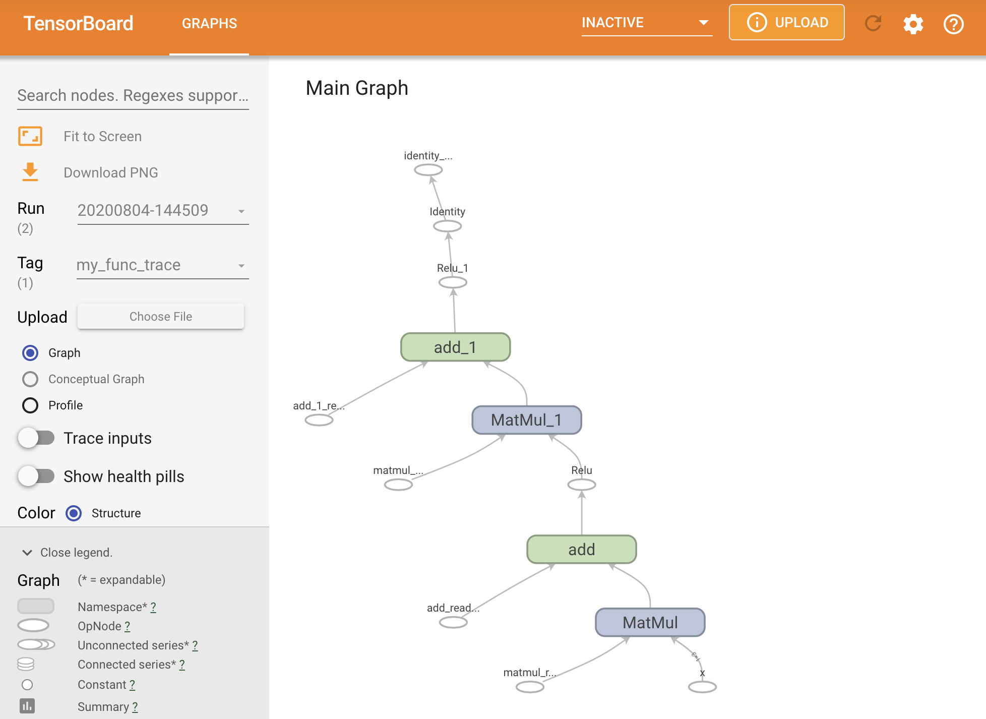
You can visualize the graph by tracing it within a TensorBoard summary.
# Set up logging.
stamp = datetime.now().strftime("%Y%m%d-%H%M%S")
logdir = "logs/func/%s" % stamp
writer = tf.summary.create_file_writer(logdir)

# Create a new model to get a fresh trace
# Otherwise the summary will not see the graph.
new_model = MySequentialModule()

# Bracket the function call with
# tf.summary.trace_on() and tf.summary.trace_export().
tf.summary.trace_on(graph=True)
tf.profiler.experimental.start(logdir)
# Call only one tf.function when tracing.
z = print(new_model(tf.constant([[2.0, 2.0, 2.0]])))
with writer.as_default():
  tf.summary.trace_export(
      name="my_func_trace",
      step=0,
      profiler_outdir=logdir)
tf.Tensor([[0. 0.]], shape=(1, 2), dtype=float32)
Launch TensorBoard to view the resulting trace:
#docs_infra: no_execute
%tensorboard --logdir logs/func
Creating a SavedModel
The recommended way of sharing completely trained models is to use SavedModel. SavedModel contains both a collection of functions and a collection of weights.
You can save the model you have just trained as follows:
tf.saved_model.save(my_model, "the_saved_model")
INFO:tensorflow:Assets written to: the_saved_model/assets
# Inspect the SavedModel in the directoryls -l the_saved_model
total 32
drwxr-sr-x 2 kbuilder kokoro  4096 Oct 18 01:21 assets
-rw-rw-r-- 1 kbuilder kokoro    58 Oct 18 01:21 fingerprint.pb
-rw-rw-r-- 1 kbuilder kokoro 17704 Oct 18 01:21 saved_model.pb
drwxr-sr-x 2 kbuilder kokoro  4096 Oct 18 01:21 variables
# The variables/ directory contains a checkpoint of the variablesls -l the_saved_model/variables
total 8
-rw-rw-r-- 1 kbuilder kokoro 490 Oct 18 01:21 variables.data-00000-of-00001
-rw-rw-r-- 1 kbuilder kokoro 356 Oct 18 01:21 variables.index
The saved_model.pb file is a protocol buffer describing the functional tf.Graph.
Models and layers can be loaded from this representation without actually making an instance of the class that created it. This is desired in situations where you do not have (or want) a Python interpreter, such as serving at scale or on an edge device, or in situations where the original Python code is not available or practical to use.
You can load the model as new object:
new_model = tf.saved_model.load("the_saved_model")
new_model, created from loading a saved model, is an internal TensorFlow user object without any of the class knowledge. It is not of type SequentialModule.
isinstance(new_model, SequentialModule)
False
This new model works on the already-defined input signatures. You can't add more signatures to a model restored like this.
print(my_model([[2.0, 2.0, 2.0]]))
print(my_model([[[2.0, 2.0, 2.0], [2.0, 2.0, 2.0]]]))
tf.Tensor([[0.31593648 0.        ]], shape=(1, 2), dtype=float32)
tf.Tensor(
[[[0.31593648 0.        ]
  [0.31593648 0.        ]]], shape=(1, 2, 2), dtype=float32)
Thus, using SavedModel, you are able to save TensorFlow weights and graphs using tf.Module, and then load them again.
Keras models and layers
Note that up until this point, there is no mention of Keras. You can build your own high-level API on top of tf.Module, and people have.
In this section, you will examine how Keras uses tf.Module. A complete user guide to Keras models can be found in the Keras guide.
Keras layers and models have a lot more extra features including:
- Optional losses
- Support for metrics
- Built-in support for an optional
trainingargument to differentiate between training and inference use - Saving and restoring python objects instead of just black-box functions
get_configandfrom_configmethods that allow you to accurately store configurations to allow model cloning in Python
These features allow for far more complex models through subclassing, such as a custom GAN or a Variational AutoEncoder (VAE) model. Read about them in the full guide to custom layers and models.
Keras models also come with extra functionality that makes them easy to train, evaluate, load, save, and even train on multiple machines.
Keras layers
tf.keras.layers.Layer is the base class of all Keras layers, and it inherits from tf.Module.
You can convert a module into a Keras layer just by swapping out the parent and then changing __call__ to call:
class MyDense(tf.keras.layers.Layer):
  # Adding **kwargs to support base Keras layer arguments
  def __init__(self, in_features, out_features, **kwargs):
    super().__init__(**kwargs)

    # This will soon move to the build step; see below
    self.w = tf.Variable(
      tf.random.normal([in_features, out_features]), name='w')
    self.b = tf.Variable(tf.zeros([out_features]), name='b')
  def call(self, x):
    y = tf.matmul(x, self.w) + self.b
    return tf.nn.relu(y)

simple_layer = MyDense(name="simple", in_features=3, out_features=3)
Keras layers have their own __call__ that does some bookkeeping described in the next section and then calls call(). You should notice no change in functionality.
simple_layer([[2.0, 2.0, 2.0]])
<tf.Tensor: shape=(1, 3), dtype=float32, numpy=array([[1.1688161, 0. , 0. ]], dtype=float32)>
The build step
As noted, it's convenient in many cases to wait to create variables until you are sure of the input shape.
Keras layers come with an extra lifecycle step that allows you more flexibility in how you define your layers. This is defined in the build function.
build is called exactly once, and it is called with the shape of the input. It's usually used to create variables (weights).
You can rewrite MyDense layer above to be flexible to the size of its inputs:
class FlexibleDense(tf.keras.layers.Layer):
  # Note the added `**kwargs`, as Keras supports many arguments
  def __init__(self, out_features, **kwargs):
    super().__init__(**kwargs)
    self.out_features = out_features

  def build(self, input_shape):  # Create the state of the layer (weights)
    self.w = tf.Variable(
      tf.random.normal([input_shape[-1], self.out_features]), name='w')
    self.b = tf.Variable(tf.zeros([self.out_features]), name='b')

  def call(self, inputs):  # Defines the computation from inputs to outputs
    return tf.matmul(inputs, self.w) + self.b

# Create the instance of the layer
flexible_dense = FlexibleDense(out_features=3)
At this point, the model has not been built, so there are no variables:
flexible_dense.variables
[]
Calling the function allocates appropriately-sized variables:
# Call it, with predictably random results
print("Model results:", flexible_dense(tf.constant([[2.0, 2.0, 2.0], [3.0, 3.0, 3.0]])))
Model results: tf.Tensor(
[[-2.531786  -5.5550847 -0.4248762]
 [-3.7976792 -8.332626  -0.6373143]], shape=(2, 3), dtype=float32)
flexible_dense.variables
[<tf.Variable 'flexible_dense/w:0' shape=(3, 3) dtype=float32, numpy=
 array([[-0.77719826, -1.9281565 ,  0.82326293],
        [ 0.85628736, -0.31845194,  0.10916236],
        [-1.3449821 , -0.5309338 , -1.1448634 ]], dtype=float32)>,
 <tf.Variable 'flexible_dense/b:0' shape=(3,) dtype=float32, numpy=array([0., 0., 0.], dtype=float32)>]
Since build is only called once, inputs will be rejected if the input shape is not compatible with the layer's variables:
try:
  print("Model results:", flexible_dense(tf.constant([[2.0, 2.0, 2.0, 2.0]])))
except tf.errors.InvalidArgumentError as e:
  print("Failed:", e)
Failed: Exception encountered when calling layer 'flexible_dense' (type FlexibleDense).

{ {function_node __wrapped__MatMul_device_/job:localhost/replica:0/task:0/device:CPU:0} } Matrix size-incompatible: In[0]: [1,4], In[1]: [3,3] [Op:MatMul] name:

Call arguments received by layer 'flexible_dense' (type FlexibleDense):
  • inputs=tf.Tensor(shape=(1, 4), dtype=float32)
Keras models
You can define your model as nested Keras layers.
However, Keras also provides a full-featured model class called tf.keras.Model. It inherits from tf.keras.layers.Layer, so a Keras model can be used and nested in the same way as Keras layers. Keras models come with extra functionality that makes them easy to train, evaluate, load, save, and even train on multiple machines.
You can define the SequentialModule from above with nearly identical code, again converting __call__ to call() and changing the parent:
@keras.saving.register_keras_serializable()
class MySequentialModel(tf.keras.Model):
  def __init__(self, name=None, **kwargs):
    super().__init__(**kwargs)

    self.dense_1 = FlexibleDense(out_features=3)
    self.dense_2 = FlexibleDense(out_features=2)
  def call(self, x):
    x = self.dense_1(x)
    return self.dense_2(x)

# You have made a Keras model!
my_sequential_model = MySequentialModel(name="the_model")

# Call it on a tensor, with random results
print("Model results:", my_sequential_model(tf.constant([[2.0, 2.0, 2.0]])))
Model results: tf.Tensor([[ 0.26034355 16.431221 ]], shape=(1, 2), dtype=float32)
All the same features are available, including tracking variables and submodules.
my_sequential_model.variables
[<tf.Variable 'my_sequential_model/flexible_dense_1/w:0' shape=(3, 3) dtype=float32, numpy=
 array([[ 1.4749854 ,  0.16090827,  2.2669017 ],
        [ 1.6850946 ,  1.1545411 ,  0.1707306 ],
        [ 0.8753734 , -0.13549292,  0.08751986]], dtype=float32)>,
 <tf.Variable 'my_sequential_model/flexible_dense_1/b:0' shape=(3,) dtype=float32, numpy=array([0., 0., 0.], dtype=float32)>,
 <tf.Variable 'my_sequential_model/flexible_dense_2/w:0' shape=(3, 2) dtype=float32, numpy=
 array([[-0.8022977 ,  1.9773549 ],
        [-0.76657015, -0.8485579 ],
        [ 1.6919082 ,  0.49000967]], dtype=float32)>,
 <tf.Variable 'my_sequential_model/flexible_dense_2/b:0' shape=(2,) dtype=float32, numpy=array([0., 0.], dtype=float32)>]
my_sequential_model.submodules
(<__main__.FlexibleDense at 0x7f790c7e0e80>,
 <__main__.FlexibleDense at 0x7f790c7e6940>)
Overriding tf.keras.Model is a very Pythonic approach to building TensorFlow models. If you are migrating models from other frameworks, this can be very straightforward.
If you are constructing models that are simple assemblages of existing layers and inputs, you can save time and space by using the functional API, which comes with additional features around model reconstruction and architecture.
Here is the same model with the functional API:
inputs = tf.keras.Input(shape=[3,])

x = FlexibleDense(3)(inputs)
x = FlexibleDense(2)(x)

my_functional_model = tf.keras.Model(inputs=inputs, outputs=x)

my_functional_model.summary()
Model: "model"
_________________________________________________________________
 Layer (type)                Output Shape              Param #
=================================================================
 input_1 (InputLayer)        [(None, 3)]               0

 flexible_dense_3 (Flexible  (None, 3)                 12
 Dense)

 flexible_dense_4 (Flexible  (None, 2)                 8
 Dense)

=================================================================
Total params: 20 (80.00 Byte)
Trainable params: 20 (80.00 Byte)
Non-trainable params: 0 (0.00 Byte)
_________________________________________________________________
my_functional_model(tf.constant([[2.0, 2.0, 2.0]]))
<tf.Tensor: shape=(1, 2), dtype=float32, numpy=array([[3.4276495, 2.937252 ]], dtype=float32)>
The major difference here is that the input shape is specified up front as part of the functional construction process. The input_shape argument in this case does not have to be completely specified; you can leave some dimensions as None.
Saving Keras models
Keras models have their own specialized zip archive saving format, marked by the .keras extension. When calling tf.keras.Model.save, add a .keras extension to the filename. For example:
my_sequential_model.save("exname_of_file.keras")
Just as easily, they can be loaded back in:
reconstructed_model = tf.keras.models.load_model("exname_of_file.keras")
Keras zip archives — .keras files — also save metric, loss, and optimizer states.
This reconstructed model can be used and will produce the same result when called on the same data:
reconstructed_model(tf.constant([[2.0, 2.0, 2.0]]))
<tf.Tensor: shape=(1, 2), dtype=float32, numpy=array([[ 0.26034355, 16.431221 ]], dtype=float32)>
Checkpointing Keras models
Keras models can also be checkpointed, and that will look the same as tf.Module.
There is more to know about saving and serialization of Keras models, including providing configuration methods for custom layers for feature support. Check out the guide to saving and serialization.
What's next
If you want to know more details about Keras, you can follow the existing Keras guides here.
Another example of a high-level API built on tf.module is Sonnet from DeepMind, which is covered on their site.