| | |  Lihat di GitHub Lihat di GitHub | | |
YAMNet adalah jaring yang mendalam yang memprediksi 521 event audio yang kelas dari corpus AudioSet-YouTube itu dilatih. Ini mempekerjakan Mobilenet_v1 depthwise-dipisahkan arsitektur belit.
import tensorflow as tf
import tensorflow_hub as hub
import numpy as np
import csv

import matplotlib.pyplot as plt
from IPython.display import Audio
from scipy.io import wavfile
Muat Model dari TensorFlow Hub.
# Load the model.
model = hub.load('https://tfhub.dev/google/yamnet/1')
Label file akan dimuat dari aset model dan hadir di model.class_map_path() . Anda akan memuatnya di class_names variabel.
# Find the name of the class with the top score when mean-aggregated across frames.
def class_names_from_csv(class_map_csv_text):
  """Returns list of class names corresponding to score vector."""
  class_names = []
  with tf.io.gfile.GFile(class_map_csv_text) as csvfile:
    reader = csv.DictReader(csvfile)
    for row in reader:
      class_names.append(row['display_name'])

  return class_names

class_map_path = model.class_map_path().numpy()
class_names = class_names_from_csv(class_map_path)
Tambahkan metode untuk memverifikasi dan mengonversi audio yang dimuat berada pada sample_rate yang tepat (16K), jika tidak maka akan memengaruhi hasil model.
def ensure_sample_rate(original_sample_rate, waveform,
                       desired_sample_rate=16000):
  """Resample waveform if required."""
  if original_sample_rate != desired_sample_rate:
    desired_length = int(round(float(len(waveform)) /
                               original_sample_rate * desired_sample_rate))
    waveform = scipy.signal.resample(waveform, desired_length)
  return desired_sample_rate, waveform
Mengunduh dan menyiapkan file suara
Di sini Anda akan mengunduh file wav dan mendengarkannya. Jika Anda memiliki file yang sudah tersedia, cukup unggah ke colab dan gunakan sebagai gantinya.
curl -O https://storage.googleapis.com/audioset/speech_whistling2.wav
% Total    % Received % Xferd  Average Speed   Time    Time     Time  Current
                                 Dload  Upload   Total   Spent    Left  Speed
100  153k  100  153k    0     0   267k      0 --:--:-- --:--:-- --:--:--  266k
curl -O https://storage.googleapis.com/audioset/miaow_16k.wav
% Total    % Received % Xferd  Average Speed   Time    Time     Time  Current
                                 Dload  Upload   Total   Spent    Left  Speed
100  210k  100  210k    0     0   185k      0  0:00:01  0:00:01 --:--:--  185k
# wav_file_name = 'speech_whistling2.wav'
wav_file_name = 'miaow_16k.wav'
sample_rate, wav_data = wavfile.read(wav_file_name, 'rb')
sample_rate, wav_data = ensure_sample_rate(sample_rate, wav_data)

# Show some basic information about the audio.
duration = len(wav_data)/sample_rate
print(f'Sample rate: {sample_rate} Hz')
print(f'Total duration: {duration:.2f}s')
print(f'Size of the input: {len(wav_data)}')

# Listening to the wav file.
Audio(wav_data, rate=sample_rate)
Sample rate: 16000 Hz
Total duration: 6.73s
Size of the input: 107698
/tmpfs/src/tf_docs_env/lib/python3.7/site-packages/ipykernel_launcher.py:3: WavFileWarning: Chunk (non-data) not understood, skipping it.
  This is separate from the ipykernel package so we can avoid doing imports until
The wav_data kebutuhan akan dinormalisasi dengan nilai-nilai di [-1.0, 1.0] (sebagaimana tercantum dalam model dokumentasi ).
waveform = wav_data / tf.int16.max
Menjalankan Model
Sekarang bagian yang mudah: menggunakan data yang sudah disiapkan, Anda cukup memanggil model dan mendapatkan: skor, embedding, dan spektogram.
Skor adalah hasil utama yang akan Anda gunakan. Spektogram yang akan Anda gunakan untuk melakukan beberapa visualisasi nanti.
# Run the model, check the output.
scores, embeddings, spectrogram = model(waveform)
scores_np = scores.numpy()
spectrogram_np = spectrogram.numpy()
infered_class = class_names[scores_np.mean(axis=0).argmax()]
print(f'The main sound is: {infered_class}')
The main sound is: Animal
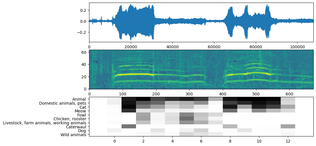
visualisasi
YAMNet juga mengembalikan beberapa informasi tambahan yang dapat kita gunakan untuk visualisasi. Mari kita lihat pada Waveform, spektogram dan kelas teratas yang disimpulkan.
plt.figure(figsize=(10, 6))

# Plot the waveform.
plt.subplot(3, 1, 1)
plt.plot(waveform)
plt.xlim([0, len(waveform)])

# Plot the log-mel spectrogram (returned by the model).
plt.subplot(3, 1, 2)
plt.imshow(spectrogram_np.T, aspect='auto', interpolation='nearest', origin='lower')

# Plot and label the model output scores for the top-scoring classes.
mean_scores = np.mean(scores, axis=0)
top_n = 10
top_class_indices = np.argsort(mean_scores)[::-1][:top_n]
plt.subplot(3, 1, 3)
plt.imshow(scores_np[:, top_class_indices].T, aspect='auto', interpolation='nearest', cmap='gray_r')

# patch_padding = (PATCH_WINDOW_SECONDS / 2) / PATCH_HOP_SECONDS
# values from the model documentation
patch_padding = (0.025 / 2) / 0.01
plt.xlim([-patch_padding-0.5, scores.shape[0] + patch_padding-0.5])
# Label the top_N classes.
yticks = range(0, top_n, 1)
plt.yticks(yticks, [class_names[top_class_indices[x]] for x in yticks])
_ = plt.ylim(-0.5 + np.array([top_n, 0]))