# FFJORD

|---|---|---|---|
| [![](https://www.tensorflow.org/images/tf_logo_32px.png)View on TensorFlow.org](https://www.tensorflow.org/probability/examples/FFJORD_Demo) | [![](https://www.tensorflow.org/images/colab_logo_32px.png)Run in Google Colab](https://colab.research.google.com/github/tensorflow/probability/blob/main/tensorflow_probability/examples/jupyter_notebooks/FFJORD_Demo.ipynb) | [![](https://www.tensorflow.org/images/GitHub-Mark-32px.png)View source on GitHub](https://github.com/tensorflow/probability/blob/main/tensorflow_probability/examples/jupyter_notebooks/FFJORD_Demo.ipynb) | [![](https://www.tensorflow.org/images/download_logo_32px.png)Download notebook](https://storage.googleapis.com/tensorflow_docs/probability/tensorflow_probability/examples/jupyter_notebooks/FFJORD_Demo.ipynb) |

## Setup

First install packages used in this demo.

    pip install -q dm-sonnet

### Imports (tf, tfp with adjoint trick, etc)

<br />

<button type="button" class="button-red button expand-control">Toggle code</button>

<br />

    import numpy as np
    import tqdm as tqdm
    import sklearn.datasets as skd

    # visualization
    import matplotlib.pyplot as plt
    import seaborn as sns
    from scipy.stats import kde

    # tf and friends
    import tensorflow.compat.v2 as tf
    import tensorflow_probability as tfp
    import sonnet as snt
    tf.enable_v2_behavior()

    tfb = tfp.bijectors
    tfd = tfp.distributions

    def make_grid(xmin, xmax, ymin, ymax, gridlines, pts):
      xpts = np.linspace(xmin, xmax, pts)
      ypts = np.linspace(ymin, ymax, pts)
      xgrid = np.linspace(xmin, xmax, gridlines)
      ygrid = np.linspace(ymin, ymax, gridlines)
      xlines = np.stack([a.ravel() for a in np.meshgrid(xpts, ygrid)])
      ylines = np.stack([a.ravel() for a in np.meshgrid(xgrid, ypts)])
      return np.concatenate([xlines, ylines], 1).T

    grid = make_grid(-3, 3, -3, 3, 4, 100)

<br />

<br />

```
/usr/local/lib/python3.6/dist-packages/statsmodels/tools/_testing.py:19: FutureWarning: pandas.util.testing is deprecated. Use the functions in the public API at pandas.testing instead.
  import pandas.util.testing as tm
```

### Helper functions for visualization

<br />

<button type="button" class="button-red button expand-control">Toggle code</button>

<br />

    def plot_density(data, axis):
      x, y = np.squeeze(np.split(data, 2, axis=1))
      levels = np.linspace(0.0, 0.75, 10)
      kwargs = {'levels': levels}
      return sns.kdeplot(x, y, cmap="viridis", shade=True, 
                         shade_lowest=True, ax=axis, **kwargs)


    def plot_points(data, axis, s=10, color='b', label=''):
      x, y = np.squeeze(np.split(data, 2, axis=1))
      axis.scatter(x, y, c=color, s=s, label=label)


    def plot_panel(
        grid, samples, transformed_grid, transformed_samples,
        dataset, axarray, limits=True):
      if len(axarray) != 4:
        raise ValueError('Expected 4 axes for the panel')
      ax1, ax2, ax3, ax4 = axarray
      plot_points(data=grid, axis=ax1, s=20, color='black', label='grid')
      plot_points(samples, ax1, s=30, color='blue', label='samples')
      plot_points(transformed_grid, ax2, s=20, color='black', label='ode(grid)')
      plot_points(transformed_samples, ax2, s=30, color='blue', label='ode(samples)')
      ax3 = plot_density(transformed_samples, ax3)
      ax4 = plot_density(dataset, ax4)
      if limits:
        set_limits([ax1], -3.0, 3.0, -3.0, 3.0)
        set_limits([ax2], -2.0, 3.0, -2.0, 3.0)
        set_limits([ax3, ax4], -1.5, 2.5, -0.75, 1.25)


    def set_limits(axes, min_x, max_x, min_y, max_y):
      if isinstance(axes, list):
        for axis in axes:
          set_limits(axis, min_x, max_x, min_y, max_y)
      else:
        axes.set_xlim(min_x, max_x)
        axes.set_ylim(min_y, max_y)

<br />

<br />

# FFJORD bijector

In this colab we demonstrate FFJORD bijector, originally proposed in the paper by Grathwohl, Will, et al. [arxiv link](https://arxiv.org/pdf/1810.01367.pdf).

In the nutshell the idea behind such approach is to establish a correspondence between a known **base distribution** and the **data distribution**.

To establish this connection, we need to

1. Define a bijective map \\(\\mathcal{T}_{\\theta}:\\mathbf{x} \\rightarrow \\mathbf{y}\\), \\(\\mathcal{T}_{\\theta}\^{1}:\\mathbf{y} \\rightarrow \\mathbf{x}\\) between the space \\(\\mathcal{Y}\\) on which **base distribution** is defined and space \\(\\mathcal{X}\\) of the data domain.
2. Efficiently keep track of the deformations we perform to transfer the notion of probability onto \\(\\mathcal{X}\\).

The second condition is formalized in the following expression for probability
distribution defined on \\(\\mathcal{X}\\):

\\\[
\\log p_{\\mathbf{x} }(\\mathbf{x})=\\log p_{\\mathbf{y} }(\\mathbf{y})-\\log \\operatorname{det}\\left\|\\frac{\\partial \\mathcal{T}_{\\theta}(\\mathbf{y})}{\\partial \\mathbf{y} }\\right\|
\\\]

FFJORD bijector accomplishes this by defining a transformation

\\\[
\\mathcal{T_{\\theta} }: \\mathbf{x} = \\mathbf{z}(t_{0}) \\rightarrow \\mathbf{y} = \\mathbf{z}(t_{1}) \\quad : \\quad \\frac{d \\mathbf{z} }{dt} = \\mathbf{f}(t, \\mathbf{z}, \\theta)
\\\]

This transformation is invertible, as long as function \\(\\mathbf{f}\\) describing the evolution of the state \\(\\mathbf{z}\\) is well behaved and the `log_det_jacobian` can be calculated by integrating the following expression.

\\\[
\\log \\operatorname{det}\\left\|\\frac{\\partial \\mathcal{T}_{\\theta}(\\mathbf{y})}{\\partial \\mathbf{y} }\\right\| =
-\\int_{t_{0} }\^{t_{1} } \\operatorname{Tr}\\left(\\frac{\\partial \\mathbf{f}(t, \\mathbf{z}, \\theta)}{\\partial \\mathbf{z}(t)}\\right) d t
\\\]

In this demo we will train a FFJORD bijector to warp a gaussian distribution onto the distribution defined by `moons` dataset. This will be done in 3 steps:

- Define **base distribution**
- Define FFJORD bijector
- Minimize exact log-likelihood of the dataset

First, we load the data

### Dataset
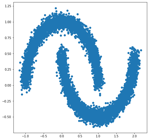
<br />

<button type="button" class="button-red button expand-control">Toggle code</button>

<br />

    DATASET_SIZE = 1024 * 8 
    BATCH_SIZE = 256 
    SAMPLE_SIZE = DATASET_SIZE

    moons = skd.make_moons(n_samples=DATASET_SIZE, noise=.06)[0]

    moons_ds = tf.data.Dataset.from_tensor_slices(moons.astype(np.float32))
    moons_ds = moons_ds.prefetch(tf.data.experimental.AUTOTUNE)
    moons_ds = moons_ds.cache()
    moons_ds = moons_ds.shuffle(DATASET_SIZE)
    moons_ds = moons_ds.batch(BATCH_SIZE)

    plt.figure(figsize=[8, 8])
    plt.scatter(moons[:, 0], moons[:, 1])
    plt.show()

<br />

<br />

![png](https://www.tensorflow.org/static/probability/examples/FFJORD_Demo_files/output_aWk3YD4zWx_b_0.png)

Next, we instantiate a base distribution

    base_loc = np.array([0.0, 0.0]).astype(np.float32)
    base_sigma = np.array([0.8, 0.8]).astype(np.float32)
    base_distribution = tfd.MultivariateNormalDiag(base_loc, base_sigma)

We use a multi-layer perceptron to model `state_derivative_fn`.

While not necessary for this dataset, it is often benefitial to make `state_derivative_fn` dependent on time. Here we achieve this by concatenating `t` to inputs of our network.

    class MLP_ODE(snt.Module):
      """Multi-layer NN ode_fn."""
      def __init__(self, num_hidden, num_layers, num_output, name='mlp_ode'):
        super(MLP_ODE, self).__init__(name=name)
        self._num_hidden = num_hidden
        self._num_output = num_output
        self._num_layers = num_layers
        self._modules = []
        for _ in range(self._num_layers - 1):
          self._modules.append(snt.Linear(self._num_hidden))
          self._modules.append(tf.math.tanh)
        self._modules.append(snt.Linear(self._num_output))
        self._model = snt.Sequential(self._modules)

      def __call__(self, t, inputs):
        inputs = tf.concat([tf.broadcast_to(t, inputs.shape), inputs], -1)
        return self._model(inputs)

### Model and training parameters

<br />

<button type="button" class="button-red button expand-control">Toggle code</button>

<br />

    LR = 1e-2 
    NUM_EPOCHS = 80 
    STACKED_FFJORDS = 4 
    NUM_HIDDEN = 8 
    NUM_LAYERS = 3 
    NUM_OUTPUT = 2

<br />

<br />

Now we construct a stack of FFJORD bijectors. Each bijector is provided with `ode_solve_fn` and `trace_augmentation_fn` and it's own `state_derivative_fn` model, so that they represent a sequence of different transformations.

### Building bijector

<br />

<button type="button" class="button-red button expand-control">Toggle code</button>

<br />

    solver = tfp.math.ode.DormandPrince(atol=1e-5)
    ode_solve_fn = solver.solve
    trace_augmentation_fn = tfb.ffjord.trace_jacobian_exact

    bijectors = []
    for _ in range(STACKED_FFJORDS):
      mlp_model = MLP_ODE(NUM_HIDDEN, NUM_LAYERS, NUM_OUTPUT)
      next_ffjord = tfb.FFJORD(
          state_time_derivative_fn=mlp_model,ode_solve_fn=ode_solve_fn,
          trace_augmentation_fn=trace_augmentation_fn)
      bijectors.append(next_ffjord)

    stacked_ffjord = tfb.Chain(bijectors[::-1])

<br />

<br />

Now we can use `TransformedDistribution` which is the result of warping `base_distribution` with `stacked_ffjord` bijector.

    transformed_distribution = tfd.TransformedDistribution(
        distribution=base_distribution, bijector=stacked_ffjord)

Now we define our training procedure. We simply minimize negative log-likelihood of the data.

### Training

<br />

<button type="button" class="button-red button expand-control">Toggle code</button>

<br />

    @tf.function
    def train_step(optimizer, target_sample):
      with tf.GradientTape() as tape:
        loss = -tf.reduce_mean(transformed_distribution.log_prob(target_sample))
      variables = tape.watched_variables()
      gradients = tape.gradient(loss, variables)
      optimizer.apply(gradients, variables)
      return loss

<br />

<br />

### Samples

<br />

<button type="button" class="button-red button expand-control">Toggle code</button>

<br />

    @tf.function
    def get_samples():
      base_distribution_samples = base_distribution.sample(SAMPLE_SIZE)
      transformed_samples = transformed_distribution.sample(SAMPLE_SIZE)
      return base_distribution_samples, transformed_samples


    @tf.function
    def get_transformed_grid():
      transformed_grid = stacked_ffjord.forward(grid)
      return transformed_grid

<br />

<br />

Plot samples from base and transformed distributions.

    evaluation_samples = []
    base_samples, transformed_samples = get_samples()
    transformed_grid = get_transformed_grid()
    evaluation_samples.append((base_samples, transformed_samples, transformed_grid))

```
WARNING:tensorflow:From /usr/local/lib/python3.6/dist-packages/tensorflow/python/ops/resource_variable_ops.py:1817: calling BaseResourceVariable.__init__ (from tensorflow.python.ops.resource_variable_ops) with constraint is deprecated and will be removed in a future version.
Instructions for updating:
If using Keras pass *_constraint arguments to layers.
```

    panel_id = 0
    panel_data = evaluation_samples[panel_id]
    fig, axarray = plt.subplots(
      1, 4, figsize=(16, 6))
    plot_panel(
        grid, panel_data[0], panel_data[2], panel_data[1], moons, axarray, False)
    plt.tight_layout()

![png](https://www.tensorflow.org/static/probability/examples/FFJORD_Demo_files/output_CQyH94U1Xh_O_0.png)

    learning_rate = tf.Variable(LR, trainable=False)
    optimizer = snt.optimizers.Adam(learning_rate)

    for epoch in tqdm.trange(NUM_EPOCHS // 2):
      base_samples, transformed_samples = get_samples()
      transformed_grid = get_transformed_grid()
      evaluation_samples.append(
          (base_samples, transformed_samples, transformed_grid))
      for batch in moons_ds:
        _ = train_step(optimizer, batch)

```
0%|          | 0/40 [00:00<?, ?it/s]
WARNING:tensorflow:From /usr/local/lib/python3.6/dist-packages/tensorflow_probability/python/math/ode/base.py:350: calling while_loop_v2 (from tensorflow.python.ops.control_flow_ops) with back_prop=False is deprecated and will be removed in a future version.
Instructions for updating:
back_prop=False is deprecated. Consider using tf.stop_gradient instead.
Instead of:
results = tf.while_loop(c, b, vars, back_prop=False)
Use:
results = tf.nest.map_structure(tf.stop_gradient, tf.while_loop(c, b, vars))
100%|██████████| 40/40 [07:00<00:00, 10.52s/it]
```

    panel_id = -1
    panel_data = evaluation_samples[panel_id]
    fig, axarray = plt.subplots(
      1, 4, figsize=(16, 6))
    plot_panel(grid, panel_data[0], panel_data[2], panel_data[1], moons, axarray)
    plt.tight_layout()

![png](https://www.tensorflow.org/static/probability/examples/FFJORD_Demo_files/output_G2sVjn77XiJt_0.png)

Training it for longer with learning rate results in further improvements.

Not convered in this example, FFJORD bijector supports hutchinson's stochastic trace estimation. The particular estimator can be provided via `trace_augmentation_fn`. Similarly alternative integrators can be used by defining custom `ode_solve_fn`.