
| |
 在 GitHub 上查看源代码 在 GitHub 上查看源代码
|
|
线性混合效应模型是一种用于对结构化线性关系进行建模的简单方式(Harville,1997 年;Laird 和 Ware,1982 年)。每个数据点都包含不同类型的输入(分类为多个组)和实值输出。线性混合效应模型是一种分层模型:它在各个组之间共享统计强度,以便改善对任何单个数据点的推断。
在本教程中,我们以 TensorFlow Probability 中的真实示例来演示线性混合效应模型。我们将使用 JointDistributionCoroutine 和 Markov Chain Monte Carlo (tfp.mcmc) 模块。
依赖项和前提条件
Import and set ups
import csv
import matplotlib.pyplot as plt
import numpy as np
import pandas as pd
import requests

import tensorflow as tf
import tensorflow_probability as tfp

tfd = tfp.distributions
tfb = tfp.bijectors

dtype = tf.float64

%config InlineBackend.figure_format = 'retina'
%matplotlib inline
plt.style.use('ggplot')
加快速度!
在深入探究之前,请确保我们在此演示中使用 GPU。
为此,请选择“Runtime”->“Change runtime type”->“Hardware accelerator”->“GPU”。
以下代码段将验证我们是否有权访问 GPU。
if tf.test.gpu_device_name() != '/device:GPU:0':
  print('WARNING: GPU device not found.')
else:
  print('SUCCESS: Found GPU: {}'.format(tf.test.gpu_device_name()))
WARNING: GPU device not found.
注:如果由于某种原因无法访问 GPU,此 Colab 将仍然有效。(但训练将花费更长时间。)
数据
我们使用来自热门的 R 语言 lme4 软件包(Bates 等人,2015 年)中的 InstEval 数据集。它是一个课程及其评估评分的数据集。每门课程都包含元数据,例如 students、instructors 和 departments,而关注的响应变量是评估评分。
def load_insteval():
  """Loads the InstEval data set.

  It contains 73,421 university lecture evaluations by students at ETH
  Zurich with a total of 2,972 students, 2,160 professors and
  lecturers, and several student, lecture, and lecturer attributes.
  Implementation is built from the `observations` Python package.

  Returns:
    Tuple of np.ndarray `x_train` with 73,421 rows and 7 columns and
    dictionary `metadata` of column headers (feature names).
  """
  url = ('https://raw.github.com/vincentarelbundock/Rdatasets/master/csv/'
         'lme4/InstEval.csv')
  with requests.Session() as s:
    download = s.get(url)
    f = download.content.decode().splitlines()

  iterator = csv.reader(f)
  columns = next(iterator)[1:]
  x_train = np.array([row[1:] for row in iterator], dtype=np.int)
  metadata = {'columns': columns}
  return x_train, metadata
加载并预处理数据集。我们保留 20% 的数据,以便在未见过的数据点上评估拟合的模型。下面我们来呈现前几行。
data, metadata = load_insteval()
data = pd.DataFrame(data, columns=metadata['columns'])
data = data.rename(columns={'s': 'students',
                            'd': 'instructors',
                            'dept': 'departments',
                            'y': 'ratings'})
data['students'] -= 1  # start index by 0
# Remap categories to start from 0 and end at max(category).
data['instructors'] = data['instructors'].astype('category').cat.codes
data['departments'] = data['departments'].astype('category').cat.codes

train = data.sample(frac=0.8)
test = data.drop(train.index)

train.head()
<ipython-input-4-5d7a9eabeea1>:21: DeprecationWarning: `np.int` is a deprecated alias for the builtin `int`. To silence this warning, use `int` by itself. Doing this will not modify any behavior and is safe. When replacing `np.int`, you may wish to use e.g. `np.int64` or `np.int32` to specify the precision. If you wish to review your current use, check the release note link for additional information.
Deprecated in NumPy 1.20; for more details and guidance: https://numpy.org/devdocs/release/1.20.0-notes.html#deprecations
  x_train = np.array([row[1:] for row in iterator], dtype=np.int)
我们根据输入的 features 字典和对应于评分的 labels 输出来设置数据集。每个特征被编码为一个整数,每个标签(评估评分)被编码为一个浮点数。
get_value = lambda dataframe, key, dtype: dataframe[key].values.astype(dtype)
features_train = {
    k: get_value(train, key=k, dtype=np.int32)
    for k in ['students', 'instructors', 'departments', 'service']}
labels_train = get_value(train, key='ratings', dtype=np.float32)

features_test = {k: get_value(test, key=k, dtype=np.int32)
                 for k in ['students', 'instructors', 'departments', 'service']}
labels_test = get_value(test, key='ratings', dtype=np.float32)
num_students = max(features_train['students']) + 1
num_instructors = max(features_train['instructors']) + 1
num_departments = max(features_train['departments']) + 1
num_observations = train.shape[0]

print("Number of students:", num_students)
print("Number of instructors:", num_instructors)
print("Number of departments:", num_departments)
print("Number of observations:", num_observations)
Number of students: 2972
Number of instructors: 1128
Number of departments: 14
Number of observations: 58737
模型
典型的线性模型假定拥有独立性,其中的任何一对数据点都具有恒定的线性关系。在 InstEval 数据集中,观测值成组出现,每组都可能具有不同的斜率和截距。线性混合效应模型(也称为分层线性模型或多级线性模型)会捕获这种现象(Gelman 和 Hill,2006 年)。
这种现象的示例包括:
- 学生。来自学生的观测值不是独立的:有些学生可能会系统地给出较低(或较高)的演讲评分。
- 讲师。来自讲师的观测值不是独立的:我们预期能力出众的教师通常会获得良好的评分,而水平不足的教师通常会获得较差的评分。
- 院系。来自院系的观测值不是独立的:某些院系可能通常具有枯燥的资料或更严格的等级,因此其评分低于其他院系。
要捕获这种现象,回想一下,对于一个具有 \(N\times D\) 个特征 \(\mathbf{X}\) 和 \(N\) 个标签 \(\mathbf{y}\) 的数据集,线性回归假定模型
$$ \begin{equation*} \mathbf{y} = \mathbf{X}\beta + \alpha + \epsilon, \end{equation*} $$
其中包含斜率向量 \(\beta\in\mathbb{R}^D\)、截距 \(\alpha\in\mathbb{R}\) 和随机噪声 \(\epsilon\sim\text{Normal}(\mathbf{0}, \mathbf{I})\)。我们说 \(\beta\) 和 \(\alpha\) 是“固定效应”:它们是在数据点 \((x, y)\) 群体中保持不变的效应。作为一种似然,此方程的等价形式为 \(\mathbf{y} \sim \text{Normal}(\mathbf{X}\beta + \alpha, \mathbf{I})\)。为了找到拟合数据的 \(\beta\) 和 \(\alpha\) 的点估计值,可在推断过程中最大化这种似然。
线性混合效应模型将线性回归扩展为
\[ \begin{align*} \eta &\sim \text{Normal}(\mathbf{0}, \sigma^2 \mathbf{I}), \\ \mathbf{y} &= \mathbf{X}\beta + \mathbf{Z}\eta + \alpha + \epsilon. \end{align*} \]
其中包含斜率向量 \(\beta\in\mathbb{R}^P\)、截距 \(\alpha\in\mathbb{R}\) 和随机噪声 \(\epsilon\sim\text{Normal}(\mathbf{0}, \mathbf{I})\)。此外,还有一个 \(\mathbf{Z}\eta\) 项,其中 \(\mathbf{Z}\) 是一个特征矩阵,而 \(\eta\in\mathbb{R}^Q\) 是一个随机斜率的向量;\(\eta\) 呈正态分布,其方差分量参数为 \(\sigma^2\)。\(\mathbf{Z}\) 是根据新的 \(N\times P\) 矩阵 \(\mathbf{X}\) 和 \(N\times Q\) 矩阵 \(\mathbf{Z}\) 对原始的 \(N\times D\) 特征矩阵进行分区而形成的,其中 \(P + Q=D\):通过这种分区,我们可以单独使用固定效应 \(\beta\) 和隐变量 \(\eta\) 对特征分别建模。
我们说隐变量 \(\eta\) 是“随机效应”:它们是在整个群体中不断变化的效应(尽管它们在子群体中可能是不变的)。特别是,由于随机效应 \(\eta\) 的平均值为 0,因此数据标签的平均值由 \(\mathbf{X}\beta + \alpha\) 捕获。随机效应分量 \(\mathbf{Z}\eta\) 捕获数据中的变化:例如,“讲师 #54 的评分比平均值高 1.4 分”。
在本教程中,我们假定以下效应:
- 固定效应:
service。service是一个二进制协变量,对应于课程是否属于讲师的主要院系。无论我们收集多少其他数据,它的值只能为 \(0\) 和 \(1\)。 - 随机效应:
students、instructors和departments。在从课程评估评分的群体中获得更多观测值的情况下,我们可以关注新的学生、教师或院系。
在使用 R 语言编写的 lme4 软件包(Bates 等人,2015 年)的语法中,可以将此模型概括为
ratings ~ service + (1|students) + (1|instructors) + (1|departments) + 1
其中 x 表示固定效应,(1|x) 表示 x 的随机效应,而 1 表示截距项。
我们在下面将此模型实现为 JointDistribution。为了更好地支持参数跟踪(例如,我们要跟踪 model.trainable_variables 中的所有tf.Variable),我们将模型模板实现为 tf.Module。
class LinearMixedEffectModel(tf.Module):
  def __init__(self):
    # Set up fixed effects and other parameters.
    # These are free parameters to be optimized in E-steps
    self._intercept = tf.Variable(0., name="intercept")            # alpha in eq
    self._effect_service = tf.Variable(0., name="effect_service")  #  beta in eq
    self._stddev_students = tfp.util.TransformedVariable(
        1., bijector=tfb.Exp(), name="stddev_students")            # sigma in eq
    self._stddev_instructors = tfp.util.TransformedVariable(
        1., bijector=tfb.Exp(), name="stddev_instructors")         # sigma in eq
    self._stddev_departments = tfp.util.TransformedVariable(
        1., bijector=tfb.Exp(), name="stddev_departments")         # sigma in eq

  def __call__(self, features):
    model = tfd.JointDistributionSequential([
      # Set up random effects.
      tfd.MultivariateNormalDiag(
          loc=tf.zeros(num_students),
          scale_diag=self._stddev_students * tf.ones(num_students)),
      tfd.MultivariateNormalDiag(
          loc=tf.zeros(num_instructors),
          scale_diag=self._stddev_instructors * tf.ones(num_instructors)),
      tfd.MultivariateNormalDiag(
          loc=tf.zeros(num_departments),
          scale_diag=self._stddev_departments * tf.ones(num_departments)),
      # This is the likelihood for the observed.
      lambda effect_departments, effect_instructors, effect_students: tfd.Independent(
          tfd.Normal(
              loc=(self._effect_service * features["service"] +
                  tf.gather(effect_students, features["students"], axis=-1) +
                  tf.gather(effect_instructors, features["instructors"], axis=-1) +
                  tf.gather(effect_departments, features["departments"], axis=-1) +
                  self._intercept),
              scale=1.),
              reinterpreted_batch_ndims=1)
    ])

    # To enable tracking of the trainable variables via the created distribution,
    # we attach a reference to `self`. Since all TFP objects sub-class
    # `tf.Module`, this means that the following is possible:
    # LinearMixedEffectModel()(features_train).trainable_variables
    # ==> tuple of all tf.Variables created by LinearMixedEffectModel.
    model._to_track = self
    return model

lmm_jointdist = LinearMixedEffectModel()
# Conditioned on feature/predictors from the training data
lmm_train = lmm_jointdist(features_train)
lmm_train.trainable_variables
(<tf.Variable 'effect_service:0' shape=() dtype=float32, numpy=0.0>,
 <tf.Variable 'intercept:0' shape=() dtype=float32, numpy=0.0>,
 <tf.Variable 'stddev_departments:0' shape=() dtype=float32, numpy=0.0>,
 <tf.Variable 'stddev_instructors:0' shape=() dtype=float32, numpy=0.0>,
 <tf.Variable 'stddev_students:0' shape=() dtype=float32, numpy=0.0>)
作为一种概率计算图程序,我们还可以根据计算图来呈现模型的结构。此计算图对程序中随机变量之间的数据流进行编码,从而在计算图模型方面明确它们之间的关系(Jordan,2003 年)。
作为一种统计工具,我们可以查看计算图来更好地了解情况,例如,intercept 和 effect_service 是有条件依赖的给定 ratings;如果编写的程序包含类、跨模块的交叉引用和/或子例程,则很难从源代码中看到这一点。作为一种计算工具,我们可能还会注意到隐变量通过 tf.gather 运算流入 ratings 变量。如果为 Tensor 建立索引需要大量资源,这可能是某些硬件加速器的瓶颈;通过呈现计算图,可让这一点显而易见。
lmm_train.resolve_graph()
(('effect_students', ()),
 ('effect_instructors', ()),
 ('effect_departments', ()),
 ('x', ('effect_departments', 'effect_instructors', 'effect_students')))
参数估计
给定数据后,推断的目标是拟合模型的固定效应斜率 \(\beta\)、截距 \(\alpha\) 和方差分量参数 \(\sigma^2\)。最大似然原理将此任务公式化为
$$ \max_{\beta, \alpha, \sigma}~\log p(\mathbf{y}\mid \mathbf{X}, \mathbf{Z}; \beta, \alpha, \sigma) = \max_{\beta, \alpha, \sigma}~\log \int p(\eta; \sigma) ~p(\mathbf{y}\mid \mathbf{X}, \mathbf{Z}, \eta; \beta, \alpha)~d\eta. $$
在本教程中,我们使用蒙特卡洛 EM 算法来最大化此边缘密度(Dempster 等人,1977 年;Wei 和 Tanner,1990 年)。¹ 我们执行马尔可夫链蒙特卡洛来计算条件似然相对于随机效应的期望值(“E 步骤”),随后我们执行梯度下降来最大化相对于参数的期望值(“M 步骤”):
对于 E 步骤,我们设置汉密尔顿蒙特卡洛 (HMC)。它需要一个当前状态(学生、讲师和院系效应)并返回一个新状态。我们将新状态分配给将表示 HMC 链的状态的 TensorFlow 变量。
对于 M 步骤,我们使用 HMC 的后验样本来计算边缘似然直到一个常量的无偏估计。随后,我们应用其相对于所关注参数的梯度。这会在边缘似然上产生无偏的随机下降步骤。我们使用 Adam TensorFlow 优化器来实现它,并最小化边缘的负值。
target_log_prob_fn = lambda *x: lmm_train.log_prob(x + (labels_train,))
trainable_variables = lmm_train.trainable_variables
current_state = lmm_train.sample()[:-1]
# For debugging
target_log_prob_fn(*current_state)
<tf.Tensor: shape=(), dtype=float32, numpy=-485996.53>
# Set up E-step (MCMC).
hmc = tfp.mcmc.HamiltonianMonteCarlo(
    target_log_prob_fn=target_log_prob_fn,
    step_size=0.015,
    num_leapfrog_steps=3)
kernel_results = hmc.bootstrap_results(current_state)

@tf.function(autograph=False, jit_compile=True)
def one_e_step(current_state, kernel_results):
  next_state, next_kernel_results = hmc.one_step(
      current_state=current_state,
      previous_kernel_results=kernel_results)
  return next_state, next_kernel_results

optimizer = tf.optimizers.Adam(learning_rate=.01)

# Set up M-step (gradient descent).
@tf.function(autograph=False, jit_compile=True)
def one_m_step(current_state):
  with tf.GradientTape() as tape:
    loss = -target_log_prob_fn(*current_state)
  grads = tape.gradient(loss, trainable_variables)
  optimizer.apply_gradients(zip(grads, trainable_variables))
  return loss
我们执行一个预热阶段,此阶段会运行一个 MCMC 链来进行多次迭代,以便在后验概率质量范围内初始化训练。随后,我们运行一个训练循环。此循环会联合运行 E 步骤和 M 步骤,并在训练过程中记录值。
num_warmup_iters = 1000
num_iters = 1500
num_accepted = 0
effect_students_samples = np.zeros([num_iters, num_students])
effect_instructors_samples = np.zeros([num_iters, num_instructors])
effect_departments_samples = np.zeros([num_iters, num_departments])
loss_history = np.zeros([num_iters])
# Run warm-up stage.
for t in range(num_warmup_iters):
  current_state, kernel_results = one_e_step(current_state, kernel_results)
  num_accepted += kernel_results.is_accepted.numpy()
  if t % 500 == 0 or t == num_warmup_iters - 1:
    print("Warm-Up Iteration: {:>3} Acceptance Rate: {:.3f}".format(
        t, num_accepted / (t + 1)))

num_accepted = 0  # reset acceptance rate counter

# Run training.
for t in range(num_iters):
  # run 5 MCMC iterations before every joint EM update
  for _ in range(5):
    current_state, kernel_results = one_e_step(current_state, kernel_results)
  loss = one_m_step(current_state)
  effect_students_samples[t, :] = current_state[0].numpy()
  effect_instructors_samples[t, :] = current_state[1].numpy()
  effect_departments_samples[t, :] = current_state[2].numpy()
  num_accepted += kernel_results.is_accepted.numpy()
  loss_history[t] = loss.numpy()
  if t % 500 == 0 or t == num_iters - 1:
    print("Iteration: {:>4} Acceptance Rate: {:.3f} Loss: {:.3f}".format(
        t, num_accepted / (t + 1), loss_history[t]))
Warm-Up Iteration:   0 Acceptance Rate: 1.000
Warm-Up Iteration: 500 Acceptance Rate: 0.758
Warm-Up Iteration: 999 Acceptance Rate: 0.729
Iteration:    0 Acceptance Rate: 1.000 Loss: 98200.422
Iteration:  500 Acceptance Rate: 0.649 Loss: 98190.469
Iteration: 1000 Acceptance Rate: 0.656 Loss: 98068.664
Iteration: 1499 Acceptance Rate: 0.663 Loss: 98155.070
您还可以将预热 for 循环写入 tf.while_loop,并将训练步骤写入 tf.scan 或 tf.while_loop,以实现更快的推断。例如:
@tf.function(autograph=False, jit_compile=True)
def run_k_e_steps(k, current_state, kernel_results):
  _, next_state, next_kernel_results = tf.while_loop(
      cond=lambda i, state, pkr: i < k,
      body=lambda i, state, pkr: (i+1, *one_e_step(state, pkr)),
      loop_vars=(tf.constant(0), current_state, kernel_results)
  )
  return next_state, next_kernel_results
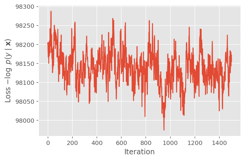
上面,我们在检测到收敛阈值后才运行算法。为了检验训练是否合理,我们验证损失函数确实在训练迭代中趋于收敛。
plt.plot(loss_history)
plt.ylabel(r'Loss $-\log$ $p(y\mid\mathbf{x})$')
plt.xlabel('Iteration')
plt.show()
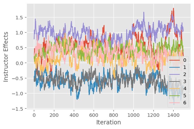
此外,我们还使用了轨迹图,它可以显示马尔可夫链蒙特卡洛算法跨特定隐维度的轨迹。在下面我们可以看到,特定讲师效应确实有意义地从其初始状态转变并探索状态空间。轨迹图还表明,不同讲师的效应有所不同,但具有相似的混合行为。
for i in range(7):
  plt.plot(effect_instructors_samples[:, i])

plt.legend([i for i in range(7)], loc='lower right')
plt.ylabel('Instructor Effects')
plt.xlabel('Iteration')
plt.show()
评论
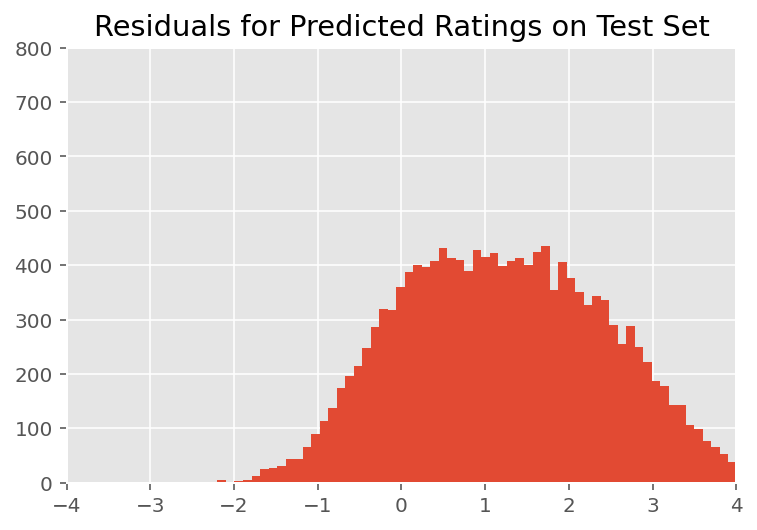
在上面,我们拟合了模型。现在,我们使用数据来评判其拟合度,这让我们可以探索并更好地理解该模型。其中一种技术是残差图,它为每个数据点绘制了模型预测值与基准真相之间的差异。如果模型正确,则它们的差异应当呈标准正态分布;图中与此模式的任何偏差都表明模型不拟合。
我们通过首先在评分上形成后验预测分布来构建残差图,这种分布会将随机效应上的先验分布替换为其后验给定训练数据。特别是,我们向前运行模型,并利用其推断的后验均值来截断它对先验随机效应的依赖。²
lmm_test = lmm_jointdist(features_test)

[
    effect_students_mean,
    effect_instructors_mean,
    effect_departments_mean,
] = [
     np.mean(x, axis=0).astype(np.float32) for x in [
       effect_students_samples,
       effect_instructors_samples,
       effect_departments_samples
       ]
]

# Get the posterior predictive distribution
(*posterior_conditionals, ratings_posterior), _ = lmm_test.sample_distributions(
    value=(
        effect_students_mean,
        effect_instructors_mean,
        effect_departments_mean,
))

ratings_prediction = ratings_posterior.mean()
从视觉上看,残差看起来有点呈标准正态分布。但是,拟合并不完美:尾部的概率质量大于正态分布,这表明模型可能会通过放宽正态性假设来提高其拟合度。
特别是,尽管在 InstEval 数据集中使用正态分布对评分建模是最常见的做法,但仔细观察数据可以发现,课程评估评分实际上是从 1 到 5 的序数值。这表明,我们应当使用有序分布,或者如果我们有足够的数据来抛弃相对排序,甚至应当使用分类分布。只需要对上述模型的一行进行更改;相同的推断代码也适用。
plt.title("Residuals for Predicted Ratings on Test Set")
plt.xlim(-4, 4)
plt.ylim(0, 800)
plt.hist(ratings_prediction - labels_test, 75)
plt.show()
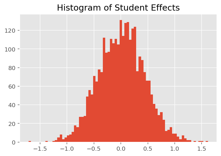
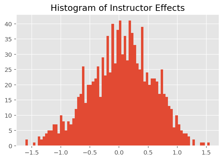
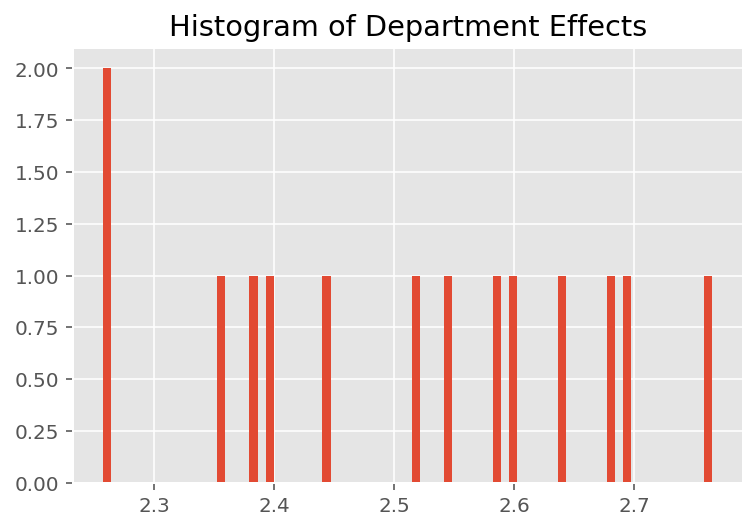
为了探索该模型如何进行各个预测,我们查看学生、讲师和院系的效应直方图。这让我们可以了解数据点的特征向量中的各个元素如何影响结果。
不出所料,我们在下面看到,每个学生对讲师的评估评分通常没有什么影响。有趣的是,我们看到讲师所属的院系具有很大的影响。
plt.title("Histogram of Student Effects")
plt.hist(effect_students_mean, 75)
plt.show()
plt.title("Histogram of Instructor Effects")
plt.hist(effect_instructors_mean, 75)
plt.show()
plt.title("Histogram of Department Effects")
plt.hist(effect_departments_mean, 75)
plt.show()
脚注
¹ 线性混合效应模型是一种我们能够以分析方式计算其边缘密度的特例。在本教程中,我们将演示蒙特卡洛 EM,它更容易应用于非分析边缘密度,例如,在将似然扩展为“分类”而不是“正态”时。
² 为简单起见,我们仅使用模型的一次前向传递来形成预测分布的均值。这是通过对后验均值进行条件处理来实现的,并且对线性混合效应模型有效。但是,这在一般情况下是无效的:后验预测分布的均值通常难以处理,并且需要在给定后验样本的情况下,在模型的多个前向传递之间取经验均值。
致谢
本教程最初用 Edward 1.0编写(源代码)。我们在此向编写和修订该版本的所有贡献者表示感谢。
参考文献
Douglas Bates and Martin Machler and Ben Bolker and Steve Walker. Fitting Linear Mixed-Effects Models Using lme4. Journal of Statistical Software, 67(1):1-48, 2015.
Arthur P. Dempster, Nan M. Laird, and Donald B. Rubin. Maximum likelihood from incomplete data via the EM algorithm. Journal of the Royal Statistical Society, Series B (Methodological), 1-38, 1977.
Andrew Gelman and Jennifer Hill. Data analysis using regression and multilevel/hierarchical models. Cambridge University Press, 2006.
David A. Harville. Maximum likelihood approaches to variance component estimation and to related problems. Journal of the American Statistical Association, 72(358):320-338, 1977.
Michael I. Jordan. An Introduction to Graphical Models. Technical Report, 2003.
Nan M. Laird and James Ware. Random-effects models for longitudinal data. Biometrics, 963-974, 1982.
Greg Wei and Martin A. Tanner. A Monte Carlo implementation of the EM algorithm and the poor man's data augmentation algorithms. Journal of the American Statistical Association, 699-704, 1990.