
La intención de este portátil es ayudar a que TFP 0.12.1 "cobre vida" a través de pequeños fragmentos: pequeñas demostraciones de cosas que puede lograr con TFP.
| | |  Ver fuente en GitHub Ver fuente en GitHub | |
Instalaciones e importaciones
!pip3 install -qU tensorflow==2.4.0 tensorflow_probability==0.12.1 tensorflow-datasets inference_gym

import tensorflow as tf
import tensorflow_probability as tfp
assert '0.12' in tfp.__version__, tfp.__version__
assert '2.4' in tf.__version__, tf.__version__

physical_devices = tf.config.list_physical_devices('CPU')
tf.config.set_logical_device_configuration(
    physical_devices[0],
    [tf.config.LogicalDeviceConfiguration(),
     tf.config.LogicalDeviceConfiguration()])

tfd = tfp.distributions
tfb = tfp.bijectors
tfpk = tfp.math.psd_kernels

import matplotlib.pyplot as plt
import numpy as np
import scipy.interpolate
import IPython
import seaborn as sns
from inference_gym import using_tensorflow as gym
import logging
Biyectores
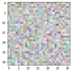
Glow
Un bijector del papel Glow: Flujo generativo con invertible 1x1 Circunvoluciones , por Kingma y Dhariwal.
A continuación se explica cómo dibujar una imagen de una distribución (tenga en cuenta que la distribución no ha "aprendido" nada aquí).
image_shape = (32, 32, 4)  # 32 x 32 RGBA image

glow = tfb.Glow(output_shape=image_shape,
                coupling_bijector_fn=tfb.GlowDefaultNetwork,
                exit_bijector_fn=tfb.GlowDefaultExitNetwork)

pz = tfd.Sample(tfd.Normal(0., 1.), tf.reduce_prod(image_shape))

# Calling glow on distribution p(z) creates our glow distribution over images.
px = glow(pz)

# Take samples from the distribution to get images from your dataset.
image = px.sample(1)[0].numpy()

# Rescale to [0, 1].
image = (image - image.min()) / (image.max() - image.min())
plt.imshow(image);
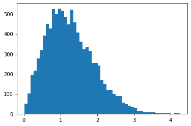
RayleighCDF
Bijector para el de distribución de Rayleigh CDF. Un uso es tomar muestras de la distribución de Rayleigh, tomando muestras uniformes y luego pasándolas por la inversa de la CDF.
bij = tfb.RayleighCDF()
uniforms = tfd.Uniform().sample(10_000)
plt.hist(bij.inverse(uniforms), bins='auto');
Ascending() reemplaza Invert(Ordered())
x = tfd.Normal(0., 1.).sample(5)
print(tfb.Ascending()(x))
print(tfb.Invert(tfb.Ordered())(x))
tf.Tensor([1.9363368 2.650928  3.4936204 4.1817293 5.6920815], shape=(5,), dtype=float32)
WARNING:tensorflow:From <ipython-input-5-1406b9939c00>:3: Ordered.__init__ (from tensorflow_probability.python.bijectors.ordered) is deprecated and will be removed after 2021-01-09.
Instructions for updating:
`Ordered` bijector is deprecated; please use `tfb.Invert(tfb.Ascending())` instead.
tf.Tensor([1.9363368 2.650928  3.4936204 4.1817293 5.6920815], shape=(5,), dtype=float32)
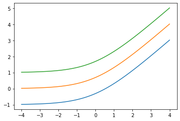
Añadir low arg: Softplus(low=2.)
x = tf.linspace(-4., 4., 100)

for low in (-1., 0., 1.):
  bij = tfb.Softplus(low=low)
  plt.plot(x, bij(x));
tfb.ScaleMatvecLinearOperatorBlock apoya en bloque LinearOperator , de varias partes args
op_1 = tf.linalg.LinearOperatorDiag(diag=[1., -1., 3.])
op_2 = tf.linalg.LinearOperatorFullMatrix([[12., 5.], [-1., 3.]])
scale = tf.linalg.LinearOperatorBlockDiag([op_1, op_2], is_non_singular=True)

bij = tfb.ScaleMatvecLinearOperatorBlock(scale)
bij([[1., 2., 3.], [0., 1.]])
WARNING:tensorflow:From /usr/local/lib/python3.6/dist-packages/tensorflow/python/ops/linalg/linear_operator_block_diag.py:223: LinearOperator.graph_parents (from tensorflow.python.ops.linalg.linear_operator) is deprecated and will be removed in a future version.
Instructions for updating:
Do not call `graph_parents`.
[<tf.Tensor: shape=(3,), dtype=float32, numpy=array([ 1., -2.,  9.], dtype=float32)>,
 <tf.Tensor: shape=(2,), dtype=float32, numpy=array([5., 3.], dtype=float32)>]
Distribuciones
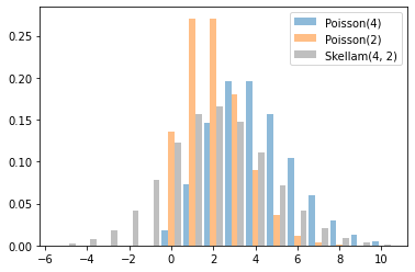
Skellam
Distribución por diferencias de dos Poisson RVs. Tenga en cuenta que las muestras de esta distribución pueden ser negativas.
x = tf.linspace(-5., 10., 10 - -5 + 1)

rates = (4, 2)
for i, rate in enumerate(rates):
  plt.bar(x - .3 * (1 - i), tfd.Poisson(rate).prob(x), label=f'Poisson({rate})', alpha=0.5, width=.3)
plt.bar(x.numpy() + .3, tfd.Skellam(*rates).prob(x).numpy(), color='k', alpha=0.25, width=.3,
        label=f'Skellam{rates}')

plt.legend();
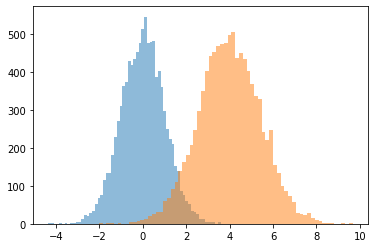
JointDistributionCoroutine[AutoBatched] productos namedtuple -como muestras
Especifique explícitamente sample_dtype=[...] para el viejo tuple comportamiento.
@tfd.JointDistributionCoroutineAutoBatched
def model():
  x = yield tfd.Normal(0., 1., name='x')
  y = x + 4.
  yield tfd.Normal(y, 1., name='y')

draw = model.sample(10_000)

plt.hist(draw.x, bins='auto', alpha=0.5)
plt.hist(draw.y, bins='auto', alpha=0.5);
WARNING:tensorflow:Note that RandomStandardNormal inside pfor op may not give same output as inside a sequential loop.
WARNING:tensorflow:Note that RandomStandardNormal inside pfor op may not give same output as inside a sequential loop.
VonMisesFisher soportes dim > 5 , entropy()
La distribución von Mises-Fisher es una distribución en la \(n-1\) esfera dimensional en \(\mathbb{R}^n\).
dist = tfd.VonMisesFisher([0., 1, 0, 1, 0, 1], concentration=1.)
draws = dist.sample(3)

print(dist.entropy())
tf.reduce_sum(draws ** 2, axis=1)  # each draw has length 1
tf.Tensor(3.3533673, shape=(), dtype=float32)
<tf.Tensor: shape=(3,), dtype=float32, numpy=array([1.0000002 , 0.99999994, 1.0000001 ], dtype=float32)>
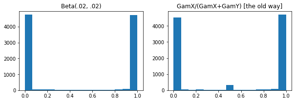
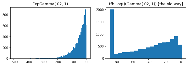
ExpGamma , ExpInverseGamma
log_rate parámetro añadido a Gamma . Mejoras numéricas cuando se toman muestras de baja concentración Beta , Dirichlet y amigos. Gradientes de reparametrización implícitos en todos los casos.
plt.figure(figsize=(10, 3))
plt.subplot(121)
plt.hist(tfd.Beta(.02, .02).sample(10_000), bins='auto')
plt.title('Beta(.02, .02)')
plt.subplot(122)
plt.title('GamX/(GamX+GamY) [the old way]')
g = tfd.Gamma(.02, 1); s0, s1 = g.sample(10_000), g.sample(10_000)
plt.hist(s0 / (s0 + s1), bins='auto')
plt.show()

plt.figure(figsize=(10, 3))
plt.subplot(121)
plt.hist(tfd.ExpGamma(.02, 1.).sample(10_000), bins='auto')
plt.title('ExpGamma(.02, 1)')
plt.subplot(122)
plt.hist(tfb.Log()(tfd.Gamma(.02, 1.)).sample(10_000), bins='auto')
plt.title('tfb.Log()(Gamma(.02, 1)) [the old way]');
JointDistribution*AutoBatched apoyar muestreo reproducible (con longitud-2 tupla / semillas Tensor)
@tfd.JointDistributionCoroutineAutoBatched
def model():
  x = yield tfd.Normal(0, 1, name='x')
  y = yield tfd.Normal(x + 4, 1, name='y')

print(model.sample(seed=(1, 2)))
print(model.sample(seed=(1, 2)))
StructTuple(
  x=<tf.Tensor: shape=(), dtype=float32, numpy=-0.59835213>,
  y=<tf.Tensor: shape=(), dtype=float32, numpy=6.2380724>
)
StructTuple(
  x=<tf.Tensor: shape=(), dtype=float32, numpy=-0.59835213>,
  y=<tf.Tensor: shape=(), dtype=float32, numpy=6.2380724>
)
KL(VonMisesFisher || SphericalUniform)
# Build vMFs with the same mean direction, batch of increasing concentrations.
vmf = tfd.VonMisesFisher(tf.math.l2_normalize(tf.random.normal([10])),
                         concentration=[0., .1, 1., 10.])
# KL increases with concentration, since vMF(conc=0) == SphericalUniform.
print(tfd.kl_divergence(vmf, tfd.SphericalUniform(10)))
tf.Tensor([4.7683716e-07 4.9877167e-04 4.9384594e-02 2.4844694e+00], shape=(4,), dtype=float32)
parameter_properties
Clases de distribución ahora exponer una parameter_properties(dtype=tf.float32, num_classes=None) método de clase, que puede permitir la construcción automatizada de muchas clases de distribuciones.
print('Gamma:', tfd.Gamma.parameter_properties())
print('Categorical:', tfd.Categorical.parameter_properties(dtype=tf.float64, num_classes=7))
Gamma: {'concentration': ParameterProperties(event_ndims=0, shape_fn=<function ParameterProperties.<lambda> at 0x7ff6bbfcdd90>, default_constraining_bijector_fn=<function Gamma._parameter_properties.<locals>.<lambda> at 0x7ff6afd95510>, is_preferred=True), 'rate': ParameterProperties(event_ndims=0, shape_fn=<function ParameterProperties.<lambda> at 0x7ff6bbfcdd90>, default_constraining_bijector_fn=<function Gamma._parameter_properties.<locals>.<lambda> at 0x7ff6afd95ea0>, is_preferred=False), 'log_rate': ParameterProperties(event_ndims=0, shape_fn=<function ParameterProperties.<lambda> at 0x7ff6bbfcdd90>, default_constraining_bijector_fn=<class 'tensorflow_probability.python.bijectors.identity.Identity'>, is_preferred=True)}
Categorical: {'logits': ParameterProperties(event_ndims=1, shape_fn=<function Categorical._parameter_properties.<locals>.<lambda> at 0x7ff6afd95510>, default_constraining_bijector_fn=<class 'tensorflow_probability.python.bijectors.identity.Identity'>, is_preferred=True), 'probs': ParameterProperties(event_ndims=1, shape_fn=<function Categorical._parameter_properties.<locals>.<lambda> at 0x7ff6afdc91e0>, default_constraining_bijector_fn=<class 'tensorflow_probability.python.bijectors.softmax_centered.SoftmaxCentered'>, is_preferred=False)}
experimental_default_event_space_bijector
Ahora acepta argumentos adicionales que fijan algunas partes de distribución.
@tfd.JointDistributionCoroutineAutoBatched
def model():
  scale = yield tfd.Gamma(1, 1, name='scale')
  obs = yield tfd.Normal(0, scale, name='obs')

model.experimental_default_event_space_bijector(obs=.2).forward(
    [tf.random.uniform([3], -2, 2.)])
StructTuple(
  scale=<tf.Tensor: shape=(3,), dtype=float32, numpy=array([0.6630705, 1.5401832, 1.0777743], dtype=float32)>
)
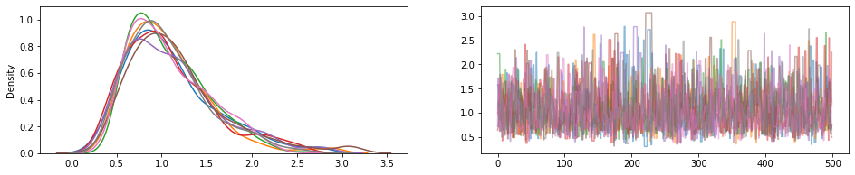
JointDistribution.experimental_pin
Botones algunas partes de distribución conjunta, que regresan JointDistributionPinned objeto que representa la densidad unnormalized articulación.
Trabajar con el experimental_default_event_space_bijector , esto hace que hacer la inferencia variacional o MCMC con los parámetros por defecto mucho más sencillo. En el siguiente ejemplo, las dos primeras líneas de sample que la ejecución de MCMC una brisa.
dist = tfd.JointDistributionSequential([
    tfd.HalfNormal(1.),
    lambda scale: tfd.Normal(0., scale, name='observed')])

@tf.function
def sample():
  bij = dist.experimental_default_event_space_bijector(observed=1.)
  target_log_prob = dist.experimental_pin(observed=1.).unnormalized_log_prob

  kernel = tfp.mcmc.TransformedTransitionKernel(
      tfp.mcmc.HamiltonianMonteCarlo(target_log_prob,
                                     step_size=0.6,
                                     num_leapfrog_steps=16),
      bijector=bij)
  return tfp.mcmc.sample_chain(500,
                               current_state=tf.ones([8]),  # multiple chains
                               kernel=kernel,
                               trace_fn=None)

draws = sample()

fig, (hist, trace) = plt.subplots(ncols=2, figsize=(16, 3))
trace.plot(draws, alpha=0.5)
for col in tf.transpose(draws):
  sns.kdeplot(col, ax=hist);
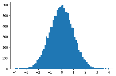
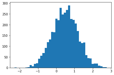
tfd.NegativeBinomial.experimental_from_mean_dispersion
Parametrización alternativa. Envíe un correo electrónico a tfprobability@tensorflow.org o envíenos un PR para agregar métodos de clase similares para otras distribuciones.
nb = tfd.NegativeBinomial.experimental_from_mean_dispersion(30., .01)
plt.hist(nb.sample(10_000), bins='auto');
tfp.experimental.distribute
DistributionStrategy -conscientes distribuciones de articulación, permitiendo para los cálculos de probabilidad en varios dispositivos. Fragmentada Independent y Sample las distribuciones.
# Note: 2-logical devices are configured in the install/import cell at top.
strategy = tf.distribute.MirroredStrategy()
assert strategy.num_replicas_in_sync == 2

@tfp.experimental.distribute.JointDistributionCoroutine
def model():
  root = tfp.experimental.distribute.JointDistributionCoroutine.Root
  group_scale = yield root(tfd.Sample(tfd.Exponential(1), 3, name='group_scale'))
  _ = yield tfp.experimental.distribute.ShardedSample(tfd.Independent(tfd.Normal(0, group_scale), 1),
                                                      sample_shape=[4], name='x')

seed1, seed2 = tfp.random.split_seed((1, 2))

@tf.function
def sample(seed):
  return model.sample(seed=seed)
xs = strategy.run(sample, (seed1,))
print("""
Note that the global latent `group_scale` is shared across devices, whereas
the local `x` is sampled independently on each device.
""")
print('sample:', xs)
print('another sample:', strategy.run(sample, (seed2,)))

@tf.function
def log_prob(x):
  return model.log_prob(x)
print("""
Note that each device observes the same log_prob (local latent log_probs are
summed across devices).
""")
print('log_prob:', strategy.run(log_prob, (xs,)))

@tf.function
def grad_log_prob(x):
  return tfp.math.value_and_gradient(model.log_prob, x)[1]

print("""
Note that each device observes the same log_prob gradient (local latents have
independent gradients, global latents have gradients aggregated across devices).
""")
print('grad_log_prob:', strategy.run(grad_log_prob, (xs,)))
WARNING:tensorflow:There are non-GPU devices in `tf.distribute.Strategy`, not using nccl allreduce.
INFO:tensorflow:Using MirroredStrategy with devices ('/job:localhost/replica:0/task:0/device:CPU:0', '/job:localhost/replica:0/task:0/device:CPU:1')

Note that the global latent `group_scale` is shared across devices, whereas
the local `x` is sampled independently on each device.

sample: StructTuple(
  group_scale=PerReplica:{
      0: <tf.Tensor: shape=(3,), dtype=float32, numpy=array([2.6355493, 1.1805456, 1.245112 ], dtype=float32)>,
      1: <tf.Tensor: shape=(3,), dtype=float32, numpy=array([2.6355493, 1.1805456, 1.245112 ], dtype=float32)>
    },
  x=PerReplica:{
      0: <tf.Tensor: shape=(2, 3), dtype=float32, numpy=
    array([[-0.90548456,  0.7675636 ,  0.27627748],
           [-0.3475989 ,  2.0194046 , -1.2531326 ]], dtype=float32)>,
      1: <tf.Tensor: shape=(2, 3), dtype=float32, numpy=
    array([[ 3.251305  , -0.5790973 ,  0.42745453],
           [-1.562331  ,  0.3006323 ,  0.635732  ]], dtype=float32)>
    }
)
another sample: StructTuple(
  group_scale=PerReplica:{
      0: <tf.Tensor: shape=(3,), dtype=float32, numpy=array([2.41133   , 0.10307606, 0.5236566 ], dtype=float32)>,
      1: <tf.Tensor: shape=(3,), dtype=float32, numpy=array([2.41133   , 0.10307606, 0.5236566 ], dtype=float32)>
    },
  x=PerReplica:{
      0: <tf.Tensor: shape=(2, 3), dtype=float32, numpy=
    array([[-3.2476294 ,  0.07213175, -0.39536062],
           [-1.2319602 , -0.05505352,  0.06356457]], dtype=float32)>,
      1: <tf.Tensor: shape=(2, 3), dtype=float32, numpy=
    array([[ 5.6028705 ,  0.11919801, -0.48446828],
           [-1.5938259 ,  0.21123725,  0.28979057]], dtype=float32)>
    }
)

Note that each device observes the same log_prob (local latent log_probs are
summed across devices).

INFO:tensorflow:Reduce to /job:localhost/replica:0/task:0/device:CPU:0 then broadcast to ('/job:localhost/replica:0/task:0/device:CPU:0', '/job:localhost/replica:0/task:0/device:CPU:1').
log_prob: PerReplica:{
  0: tf.Tensor(-25.05747, shape=(), dtype=float32),
  1: tf.Tensor(-25.05747, shape=(), dtype=float32)
}

Note that each device observes the same log_prob gradient (local latents have
independent gradients, global latents are aggregated across devices).

INFO:tensorflow:Reduce to /job:localhost/replica:0/task:0/device:CPU:0 then broadcast to ('/job:localhost/replica:0/task:0/device:CPU:0', '/job:localhost/replica:0/task:0/device:CPU:1').
INFO:tensorflow:Reduce to /job:localhost/replica:0/task:0/device:CPU:0 then broadcast to ('/job:localhost/replica:0/task:0/device:CPU:0', '/job:localhost/replica:0/task:0/device:CPU:1').
grad_log_prob: StructTuple(
  group_scale=PerReplica:{
      0: <tf.Tensor: shape=(3,), dtype=float32, numpy=array([-1.7555585, -1.2928739, -3.0554674], dtype=float32)>,
      1: <tf.Tensor: shape=(3,), dtype=float32, numpy=array([-1.7555585, -1.2928739, -3.0554674], dtype=float32)>
    },
  x=PerReplica:{
      0: <tf.Tensor: shape=(2, 3), dtype=float32, numpy=
    array([[ 0.13035832, -0.5507428 , -0.17820862],
           [ 0.05004217, -1.4489648 ,  0.80831426]], dtype=float32)>,
      1: <tf.Tensor: shape=(2, 3), dtype=float32, numpy=
    array([[-0.46807498,  0.41551432, -0.27572307],
           [ 0.22492138, -0.21570992, -0.41006932]], dtype=float32)>
    }
)
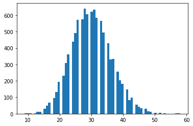
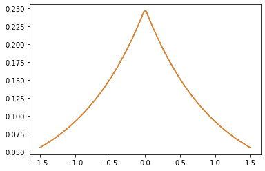
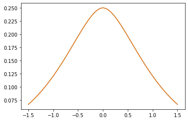
Núcleos PSD
GeneralizedMatern
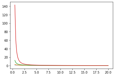
El GeneralizedMatern positiva semidefinida kernel generaliza MaternOneHalf , MAterhThreeHalves y MaternFiveHalves .
gm = tfpk.GeneralizedMatern(df=[0.5, 1.5, 2.5], length_scale=1., amplitude=0.5)
m1 = tfpk.MaternOneHalf(length_scale=1., amplitude=0.5)
m2 = tfpk.MaternThreeHalves(length_scale=1., amplitude=0.5)
m3 = tfpk.MaternFiveHalves(length_scale=1., amplitude=0.5)
xs = tf.linspace(-1.5, 1.5, 100)

gm_matrix = gm.matrix([[0.]], xs[..., tf.newaxis])
plt.plot(xs, gm_matrix[0][0])
plt.plot(xs, m1.matrix([[0.]], xs[..., tf.newaxis])[0])
plt.show()
plt.plot(xs, gm_matrix[1][0])
plt.plot(xs, m2.matrix([[0.]], xs[..., tf.newaxis])[0])
plt.show()
plt.plot(xs, gm_matrix[2][0])
plt.plot(xs, m3.matrix([[0.]], xs[..., tf.newaxis])[0])
plt.show()
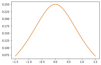
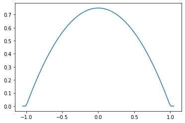
Parabolic (Epanechnikov)
epa = tfpk.Parabolic()
xs = tf.linspace(-1.05, 1.05, 100)
plt.plot(xs, epa.matrix([[0.]], xs[..., tf.newaxis])[0]);
VI
build_asvi_surrogate_posterior
Construya automáticamente un posterior sustituto estructurado para VI de manera que incorpore la estructura gráfica de la distribución previa. Este utiliza el método descrito en el documento automático estructurado variacional Inferencia ( https://arxiv.org/abs/2002.00643 ).
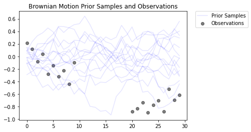
# Import a Brownian Motion model from TFP's inference gym.
model = gym.targets.BrownianMotionMissingMiddleObservations()
prior = model.prior_distribution()
ground_truth = ground_truth = model.sample_transformations['identity'].ground_truth_mean
target_log_prob = lambda *values: model.log_likelihood(values) + prior.log_prob(values)
Esto modela un proceso de movimiento browniano con un modelo de observación gaussiano. Consiste en 30 pasos de tiempo, pero los 10 pasos de tiempo del medio son inobservables.
  locs[0] ~ Normal(loc=0, scale=innovation_noise_scale)
  for t in range(1, num_timesteps):
    locs[t] ~ Normal(loc=locs[t - 1], scale=innovation_noise_scale)

  for t in range(num_timesteps):
    observed_locs[t] ~ Normal(loc=locs[t], scale=observation_noise_scale)
El objetivo es inferir los valores de locs de observaciones ruidosas ( observed_locs ). Desde los 10 timesteps medias son inobservable, observed_locs son NaN valores en timesteps [10,19].
# The observed loc values in the Brownian Motion inference gym model
OBSERVED_LOC = np.array([
    0.21592641, 0.118771404, -0.07945447, 0.037677474, -0.27885845, -0.1484156,
    -0.3250906, -0.22957903, -0.44110894, -0.09830782, np.nan, np.nan, np.nan,
    np.nan, np.nan, np.nan, np.nan, np.nan, np.nan, np.nan, -0.8786016,
    -0.83736074, -0.7384849, -0.8939254, -0.7774566, -0.70238715, -0.87771565,
    -0.51853573, -0.6948214, -0.6202789
]).astype(dtype=np.float32)

# Plot the prior and the likelihood observations
plt.figure()
plt.title('Brownian Motion Prior Samples and Observations')

num_samples = 15
prior_samples = prior.sample(num_samples)

plt.plot(prior_samples, c='blue', alpha=0.1)
plt.plot(prior_samples[0][0], label="Prior Samples", c='blue', alpha=0.1)

plt.scatter(x=range(30),y=OBSERVED_LOC, c='black', alpha=0.5, label="Observations")

plt.legend(bbox_to_anchor=(1.05, 1), borderaxespad=0.);
logging.getLogger('tensorflow').setLevel(logging.ERROR)  # suppress pfor warnings

# Construct and train an ASVI Surrogate Posterior.
asvi_surrogate_posterior = tfp.experimental.vi.build_asvi_surrogate_posterior(prior)

asvi_losses = tfp.vi.fit_surrogate_posterior(target_log_prob,
                                        asvi_surrogate_posterior,
                                        optimizer=tf.optimizers.Adam(learning_rate=0.1),
                                        num_steps=500)
logging.getLogger('tensorflow').setLevel(logging.NOTSET)
# Construct and train a Mean-Field Surrogate Posterior.
factored_surrogate_posterior = tfp.experimental.vi.build_factored_surrogate_posterior(event_shape=prior.event_shape)

factored_losses = tfp.vi.fit_surrogate_posterior(target_log_prob,
                                        factored_surrogate_posterior,
                                        optimizer=tf.optimizers.Adam(learning_rate=0.1),
                                        num_steps=500)
logging.getLogger('tensorflow').setLevel(logging.ERROR)  # suppress pfor warnings

# Sample from the posteriors.
asvi_posterior_samples = asvi_surrogate_posterior.sample(num_samples)
factored_posterior_samples = factored_surrogate_posterior.sample(num_samples)

logging.getLogger('tensorflow').setLevel(logging.NOTSET)
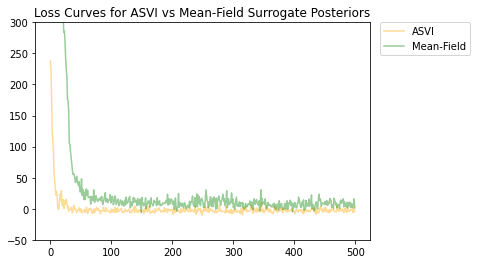
Tanto el ASVI como la distribución posterior sustituta de campo medio han convergido, y la posterior sustituta de ASVI tuvo una pérdida final menor (valor ELBO negativo).
# Plot the loss curves.
plt.figure()
plt.title('Loss Curves for ASVI vs Mean-Field Surrogate Posteriors')

plt.plot(asvi_losses, c='orange', label='ASVI', alpha = 0.4)
plt.plot(factored_losses, c='green', label='Mean-Field', alpha = 0.4)
plt.ylim(-50, 300)

plt.legend(bbox_to_anchor=(1.3, 1), borderaxespad=0.);
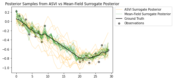
Las muestras de los posteriores resaltan lo bien que el posterior sustituto de ASVI captura la incertidumbre de los pasos de tiempo sin observaciones. Por otro lado, el posterior sustituto de campo medio lucha por capturar la verdadera incertidumbre.
# Plot samples from the ASVI and Mean-Field Surrogate Posteriors.
plt.figure()
plt.title('Posterior Samples from ASVI vs Mean-Field Surrogate Posterior')

plt.plot(asvi_posterior_samples, c='orange', alpha = 0.25)
plt.plot(asvi_posterior_samples[0][0], label='ASVI Surrogate Posterior', c='orange', alpha = 0.25)

plt.plot(factored_posterior_samples, c='green', alpha = 0.25)
plt.plot(factored_posterior_samples[0][0], label='Mean-Field Surrogate Posterior', c='green', alpha = 0.25)

plt.scatter(x=range(30),y=OBSERVED_LOC, c='black', alpha=0.5, label='Observations')

plt.plot(ground_truth, c='black', label='Ground Truth')

plt.legend(bbox_to_anchor=(1.585, 1), borderaxespad=0.);
MCMC
ProgressBarReducer
Visualice el progreso del muestreador. (Puede tener una penalización de rendimiento nominal; actualmente no es compatible con la compilación JIT).
kernel = tfp.mcmc.HamiltonianMonteCarlo(lambda x: -x**2 / 2, .05, 20)
pbar = tfp.experimental.mcmc.ProgressBarReducer(100)
kernel = tfp.experimental.mcmc.WithReductions(kernel, pbar)
plt.hist(tf.reshape(tfp.mcmc.sample_chain(100, current_state=tf.ones([128]), kernel=kernel, trace_fn=None), [-1]), bins='auto')
pbar.bar.close()
99%|█████████▉| 99/100 [00:03<00:00, 27.37it/s]
sample_sequential_monte_carlo apoya muestreo reproducible
initial_state = tf.random.uniform([4096], -2., 2.)
def smc(seed):
  return tfp.experimental.mcmc.sample_sequential_monte_carlo(
    prior_log_prob_fn=lambda x: -x**2 / 2,
    likelihood_log_prob_fn=lambda x: -(x-1.)**2 / 2,
    current_state=initial_state,
    seed=seed)[1]
plt.hist(smc(seed=(12, 34)), bins='auto');plt.show()

print(smc(seed=(12, 34))[:10])
print('different:', smc(seed=(10, 20))[:10])
print('same:', smc(seed=(12, 34))[:10])
tf.Tensor(
[ 0.665834    0.9892149   0.7961128   1.0016634  -1.000767   -0.19461267
  1.3070581   1.127177    0.9940303   0.58239716], shape=(10,), dtype=float32)
different: tf.Tensor(
[ 1.3284367   0.4374407   1.1349089   0.4557473   0.06510283 -0.08954388
  1.1735026   0.8170528   0.12443061  0.34413314], shape=(10,), dtype=float32)
same: tf.Tensor(
[ 0.665834    0.9892149   0.7961128   1.0016634  -1.000767   -0.19461267
  1.3070581   1.127177    0.9940303   0.58239716], shape=(10,), dtype=float32)
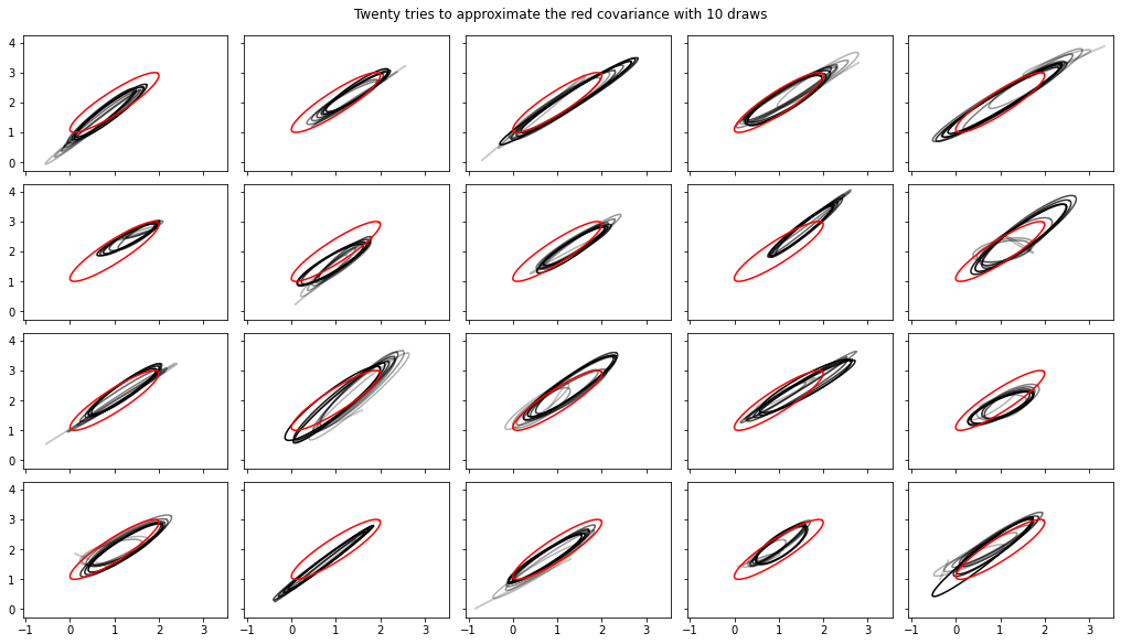
Se agregaron cálculos de transmisión de varianza, covarianza, Rhat
Nota, las interfaces con estos han cambiado algo en tfp-nightly .
def cov_to_ellipse(t, cov, mean):
  """Draw a one standard deviation ellipse from the mean, according to cov."""
  diag = tf.linalg.diag_part(cov)
  a = 0.5 * tf.reduce_sum(diag)
  b = tf.sqrt(0.25 * (diag[0] - diag[1])**2 + cov[0, 1]**2)
  major = a + b
  minor = a - b
  theta = tf.math.atan2(major - cov[0, 0], cov[0, 1])
  x = (tf.sqrt(major) * tf.cos(theta) * tf.cos(t) -
       tf.sqrt(minor) * tf.sin(theta) * tf.sin(t))
  y = (tf.sqrt(major) * tf.sin(theta) * tf.cos(t) +
       tf.sqrt(minor) * tf.cos(theta) * tf.sin(t))
  return x + mean[0], y + mean[1]

fig, axes = plt.subplots(nrows=4, ncols=5, figsize=(14, 8),
                         sharex=True, sharey=True, constrained_layout=True)
t = tf.linspace(0., 2 * np.pi, 200)
tot = 10
cov = 0.1 * tf.eye(2) + 0.9 * tf.ones([2, 2])
mvn = tfd.MultivariateNormalTriL(loc=[1., 2.],
                                 scale_tril=tf.linalg.cholesky(cov))

for ax in axes.ravel():
  rv = tfp.experimental.stats.RunningCovariance(
      num_samples=0., mean=tf.zeros(2), sum_squared_residuals=tf.zeros((2, 2)),
      event_ndims=1)

  for idx, x in enumerate(mvn.sample(tot)):
    rv = rv.update(x)
    ax.plot(*cov_to_ellipse(t, rv.covariance(), rv.mean),
            color='k', alpha=(idx + 1) / tot)
  ax.plot(*cov_to_ellipse(t, mvn.covariance(), mvn.mean()), 'r')
fig.suptitle("Twenty tries to approximate the red covariance with 10 draws");
Matemáticas, estadísticas
Funciones de Bessel: ive, kve, log-ive
xs = tf.linspace(0.5, 20., 100)
ys = tfp.math.bessel_ive([[0.5], [1.], [np.pi], [4.]], xs)
zs = tfp.math.bessel_kve([[0.5], [1.], [2.], [np.pi]], xs)

for i in range(4):
  plt.plot(xs, ys[i])
plt.show()

for i in range(4):
  plt.plot(xs, zs[i])
plt.show()
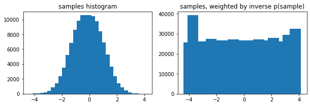
Opcionales weights Arg a tfp.stats.histogram
edges = tf.linspace(-4., 4, 31)
samps = tfd.TruncatedNormal(0, 1, -4, 4).sample(100_000, seed=(123, 456))
_, (ax1, ax2) = plt.subplots(1, 2, figsize=(10, 3))
ax1.bar(edges[:-1], tfp.stats.histogram(samps, edges))
ax1.set_title('samples histogram')
ax2.bar(edges[:-1], tfp.stats.histogram(samps, edges, weights=1 / tfd.Normal(0, 1).prob(samps)))
ax2.set_title('samples, weighted by inverse p(sample)');
tfp.math.erfcinv
x = tf.linspace(-3., 3., 10)
y = tf.math.erfc(x)
z = tfp.math.erfcinv(y)
print(x)
print(z)
tf.Tensor(
[-3.         -2.3333333  -1.6666666  -1.         -0.33333325  0.3333335

  1.          1.666667    2.3333335   3.        ], shape=(10,), dtype=float32)
tf.Tensor(
[-3.0002644  -2.3333426  -1.6666666  -0.9999997  -0.3333332   0.33333346
  0.9999999   1.6666667   2.3333335   3.0000002 ], shape=(10,), dtype=float32)