| |
 在 GitHub 上查看源代码 在 GitHub 上查看源代码
|
这是对李瑞云等人于 2020 年 3 月 16 日发表的同名论文的 TensorFlow Probability 移植。我们在 TensorFlow Probability 平台上如实地重现了原作者的方法和结果,展现了 TFP 在建立现代流行病学模型方面的一些能力。与原来的 Matlab 代码相比,移植到 TensorFlow 将模型速度提高了约 10 倍,同时,由于 TensorFlow Probability 广泛地支持向量化批次计算,因此,还可以扩展到成百上千个独立的复制性研究。
原论文
Ruiyun Li, Sen Pei, Bin Chen, Yimeng Song, Tao Zhang, Wan Yang, and Jeffrey Shaman. Substantial undocumented infection facilitates the rapid dissemination of novel coronavirus (SARS-CoV2). (2020), doi: https://doi.org/10.1126/science.abb3221 .
摘要:“Estimation of the prevalence and contagiousness of undocumented novel coronavirus (SARS-CoV2) infections is critical for understanding the overall prevalence and pandemic potential of this disease. Here we use observations of reported infection within China, in conjunction with mobility data, a networked dynamic metapopulation model and Bayesian inference, to infer critical epidemiological characteristics associated with SARS-CoV2, including the fraction of undocumented infections and their contagiousness. We estimate 86% of all infections were undocumented (95% CI: [82%–90%]) prior to 23 January 2020 travel restrictions. Per person, the transmission rate of undocumented infections was 55% of documented infections ([46%–62%]), yet, due to their greater numbers, undocumented infections were the infection source for 79% of documented cases. These findings explain the rapid geographic spread of SARS-CoV2 and indicate containment of this virus will be particularly challenging.”
代码和数据的 GitHub 链接。
概述
此模型是一个房室疾病模型,包括“易感”、“暴露”(易感染但尚无传染性)、“从未记录感染”和“最终记录感染”房室。它有两个重要特征:根据人们如何从一个城市流动到另一个城市的假设,中国的 375 个城市分别有一个单独的房室;以及感染报告会延迟,因此,在 \(t\) 日成为“最终记录感染”的病例并没有及时出现在观察到的病例统计中,而是在之后的随机某日才得到记录。
此模型假设从未记录的病例是因为症状不明显而未被记录,因此,其传染率相对较低。原论文中最重要的参数是未记录病例的比例,此参数用于评估现行感染程度,以及未记录传播对疾病传播的影响。
此 Colab 采用自下而上的方式构建代码演练。我们将按顺序执行以下操作:
- 提取并简单检查数据,
- 定义模型的状态空间和动力学,
- 按照李瑞云等人的方式为在模型中进行推断构建一组函数,以及
- 调用这些函数并检查结果。剧透:结果与论文结论一致。
安装和 Python 导入
pip3 install -q tf-nightly tfp-nightly
import collections
import io
import requests
import time
import zipfile

import matplotlib.pyplot as plt
import numpy as np
import pandas as pd

import tensorflow.compat.v2 as tf
import tensorflow_probability as tfp
from tensorflow_probability.python.internal import samplers

tfd = tfp.distributions
tfes = tfp.experimental.sequential
数据导入
从 GitHub 导入数据并检查一些数据。
r = requests.get('https://raw.githubusercontent.com/SenPei-CU/COVID-19/master/Data.zip')
z = zipfile.ZipFile(io.BytesIO(r.content))
z.extractall('/tmp/')
raw_incidence = pd.read_csv('/tmp/data/Incidence.csv')
raw_mobility = pd.read_csv('/tmp/data/Mobility.csv')
raw_population = pd.read_csv('/tmp/data/pop.csv')
我们在下面可以看到每天的原始病例统计数据。我们最感兴趣的是前 14天(从 1 月 10 日到 1 月 23 日),因为旅行限制是在 23 日实施的。该论文采用不同的参数分别对 1 月 10 日至 23 日和 1 月 23 日以后的病例数进行建模;但我们将重现重点限制在早期阶段。
raw_incidence.drop('Date', axis=1)  # The 'Date' column is all 1/18/21
# Luckily the days are in order, starting on January 10th, 2020.
我们对武汉的病例统计数据进行健全性检查。
plt.plot(raw_incidence.Wuhan, '.-')
plt.title('Wuhan incidence counts over 1/10/20 - 02/08/20')
plt.show()
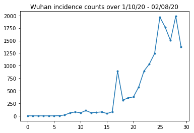
到目前为止,一切都很正常。现在查看一下最初的人口统计数据。
raw_population
我们也检查一下,并记录哪个条目是武汉。
raw_population['City'][169]
'Wuhan'
WUHAN_IDX = 169
我们在这里可以看到不同城市间的人口流动矩阵。这是前 14 天在不同城市间流动的人数的一个指标。该数据来自腾讯在 2018 年春运期间收集的 GPS 记录。李瑞云等人通过将一些未知(基于推断的)常量因子 \(\theta\) 与此数据相乘对 2020 年春运期间的人口流动建模。
raw_mobility
最后,我们将所有这些数据预处理为可以使用的 NumPy 数组。
# The given populations are only "initial" because of intercity mobility during
# the holiday season.
initial_population = raw_population['Population'].to_numpy().astype(np.float32)
将人口流动数据转换成一个形状为 [L, L, T] 的张量,其中 L 为地点数量,T 为时间步骤数量。
daily_mobility_matrices = []
for i in range(1, 15):
  day_mobility = raw_mobility[raw_mobility['Day'] == i]

  # Make a matrix of daily mobilities.
  z = pd.crosstab(
      day_mobility.Origin,
      day_mobility.Destination,
      values=day_mobility['Mobility Index'], aggfunc='sum', dropna=False)

  # Include every city, even if there are no rows for some in the raw data on
  # some day.  This uses the sort order of `raw_population`.
  z = z.reindex(index=raw_population['City'], columns=raw_population['City'],
                fill_value=0)
  # Finally, fill any missing entries with 0. This means no mobility.
  z = z.fillna(0)
  daily_mobility_matrices.append(z.to_numpy())

mobility_matrix_over_time = np.stack(daily_mobility_matrices, axis=-1).astype(
    np.float32)
最后,获取观察到的感染人数并建立一个 [L, T] 表。
# Remove the date parameter and take the first 14 days.
observed_daily_infectious_count = raw_incidence.to_numpy()[:14, 1:]
observed_daily_infectious_count = np.transpose(
    observed_daily_infectious_count).astype(np.float32)
再检查一下我们是否获得了想要的形状。提醒一下,我们处理的是 375 个城市,时间为 14 天。
print('Mobility Matrix over time should have shape (375, 375, 14): {}'.format(
    mobility_matrix_over_time.shape))
print('Observed Infectious should have shape (375, 14): {}'.format(
    observed_daily_infectious_count.shape))
print('Initial population should have shape (375): {}'.format(
    initial_population.shape))
Mobility Matrix over time should have shape (375, 375, 14): (375, 375, 14)
Observed Infectious should have shape (375, 14): (375, 14)
Initial population should have shape (375): (375,)
定义状态和参数
我们开始定义模型。我们重现的模型是 SEIR 模型的变体。在本例中,我们有下面这些时变性状态:
- \(S\):每个城市的易感人数。
- \(E\):每个城市发生过接触但尚未传染的人数。在生物学意义上,这相当于感染了这种疾病,因为所有接触过这种疾病的人最终都具有传染性。
- \(I^u\):每个城市有传染性但未记录的人数。在该模型中,这实际上是指“从未记录”。
- \(I^r\):每个城市中有传染性且已记录的人数。李瑞云等人模拟了报告延迟,因此,\(I^r\) 实际上大概是指“病例严重到足以在将来的某个时刻被记录下来”。
如下所示,我们将通过适时运行集合调整卡尔曼滤波器 (EAKF) 前馈来推断这些状态。EAKF 的状态向量是每个这些数量的一个城市索引向量。
此模型包含以下可推断的全局时变性参数:
- \(\beta\):由记录的感染病例导致的传播率。
- \(\mu\):由未记录的感染病例导致的相对传播率。这通过乘积 \(\mu \beta\) 产生作用。
- \(\theta\):城市间人口流动因数。这是一个大于 1 的因数,因为需要修正低报人口流动数据(以及从 2018 年到 2020 年的人口增长)。
- \(Z\):平均潜伏期(即,处于“暴露”状态的时间)。
- \(\alpha\):这是(最终)会被记录的严重感染病例的比例。
- \(D\):感染的平均持续时间(即,处于任何一种“感染”状态的时间)。
对于这些状态,我们将使用围绕 EAKF 的滤波迭代循环来推断这些参数的点估计值。
该模型还依赖于非推断常量:
- \(M\):城市间人口流动矩阵。此常量具有时变性,且基于推断。回想一下,它是通过推断的参数 \(\theta\) 来表示城市之间的实际人口流动。
- \(N\):每个城市的总人数。假设初始人口已知,则人口的时变由人口流动数量 \(\theta M\) 计算得出。
首先,我们设计一些数据结构来保存状态和参数。
SEIRComponents = collections.namedtuple(
  typename='SEIRComponents',
  field_names=[
    'susceptible',              # S
    'exposed',                  # E
    'documented_infectious',    # I^r
    'undocumented_infectious',  # I^u
    # This is the count of new cases in the "documented infectious" compartment.
    # We need this because we will introduce a reporting delay, between a person
    # entering I^r and showing up in the observable case count data.
    # This can't be computed from the cumulative `documented_infectious` count,
    # because some portion of that population will move to the 'recovered'
    # state, which we aren't tracking explicitly.
    'daily_new_documented_infectious'])

ModelParams = collections.namedtuple(
    typename='ModelParams',
    field_names=[
      'documented_infectious_tx_rate',             # Beta
      'undocumented_infectious_tx_relative_rate',  # Mu
      'intercity_underreporting_factor',           # Theta
      'average_latency_period',                    # Z
      'fraction_of_documented_infections',         # Alpha
      'average_infection_duration'                 # D
    ]
)
我们来为参数值编写李瑞云等人边界的代码。
PARAMETER_LOWER_BOUNDS = ModelParams(
    documented_infectious_tx_rate=0.8,
    undocumented_infectious_tx_relative_rate=0.2,
    intercity_underreporting_factor=1.,
    average_latency_period=2.,
    fraction_of_documented_infections=0.02,
    average_infection_duration=2.
)

PARAMETER_UPPER_BOUNDS = ModelParams(
    documented_infectious_tx_rate=1.5,
    undocumented_infectious_tx_relative_rate=1.,
    intercity_underreporting_factor=1.75,
    average_latency_period=5.,
    fraction_of_documented_infections=1.,
    average_infection_duration=5.
)
SEIR 动力学
我们定义参数与状态之间的关系。
李瑞云等人的时间-动力学方程式(补充材料,方程式 1-5)如下:
\(\frac{dS_i}{dt} = -\beta \frac{S_i I_i^r}{N_i} - \mu \beta \frac{S_i I_i^u}{N_i} + \theta \sum_k \frac{M_{ij} S_j}{N_j - I_j^r} - + \theta \sum_k \frac{M_{ji} S_j}{N_i - I_i^r}\)
\(\frac{dE_i}{dt} = \beta \frac{S_i I_i^r}{N_i} + \mu \beta \frac{S_i I_i^u}{N_i} -\frac{E_i}{Z} + \theta \sum_k \frac{M_{ij} E_j}{N_j - I_j^r} - + \theta \sum_k \frac{M_{ji} E_j}{N_i - I_i^r}\)
\(\frac{dI^r_i}{dt} = \alpha \frac{E_i}{Z} - \frac{I_i^r}{D}\)
\(\frac{dI^u_i}{dt} = (1 - \alpha) \frac{E_i}{Z} - \frac{I_i^u}{D} + \theta \sum_k \frac{M_{ij} I_j^u}{N_j - I_j^r} - + \theta \sum_k \frac{M_{ji} I^u_j}{N_i - I_i^r}\)
\(N_i = N_i + \theta \sum_j M_{ij} - \theta \sum_j M_{ji}\)
谨此提醒,\(i\) 和 \(j\) 下标索引城市。这些方程式基于以下方面模拟了疾病的时间演化过程:
- 与有传染性的人接触会导致更多的感染病例;
- 从“暴露”到出现一种“感染”状态的疾病进展;
- 从“感染”状态到恢复状态的疾病进展,通过从模型人口中移除来建模;
- 城市间人口流动,包括暴露或未记录感染人员;以及
- 城市间人口流动造成的日常城市人口时变性。
根据李瑞云等人的模型,我们假设严重到最终会被报告的病例不会在城市之间流动。
同样,根据李瑞云等人的模型,我们将这些动力学看作服从逐项泊松噪声,也就是说,每一项实际上是一个泊松率,即反映真实变化的样本。泊松噪声是逐项的,因为减去(而不是加上)泊松样本不会产生泊松分布的结果。
我们将使用经典的四阶龙格-库塔积分器演变这些动力学,但首先,我们来定义计算它们(包括对泊松噪声采样)的函数。
def sample_state_deltas(
    state, population, mobility_matrix, params, seed, is_deterministic=False):
  """Computes one-step change in state, including Poisson sampling.

  Note that this is coded to support vectorized evaluation on arbitrary-shape
  batches of states.  This is useful, for example, for running multiple
  independent replicas of this model to compute credible intervals for the
  parameters.  We refer to the arbitrary batch shape with the conventional
  `B` in the parameter documentation below.  This function also, of course,
  supports broadcasting over the batch shape.

  Args:
    state: A `SEIRComponents` tuple with fields Tensors of shape
      B + [num_locations] giving the current disease state.
    population: A Tensor of shape B + [num_locations] giving the current city
      populations.
    mobility_matrix: A Tensor of shape B + [num_locations, num_locations] giving
      the current baseline inter-city mobility.
    params: A `ModelParams` tuple with fields Tensors of shape B giving the
      global parameters for the current EAKF run.
    seed: Initial entropy for pseudo-random number generation.  The Poisson
      sampling is repeatable by supplying the same seed.
    is_deterministic: A `bool` flag to turn off Poisson sampling if desired.

  Returns:
    delta: A `SEIRComponents` tuple with fields Tensors of shape
      B + [num_locations] giving the one-day changes in the state, according
      to equations 1-4 above (including Poisson noise per Li et al).
  """
  undocumented_infectious_fraction = state.undocumented_infectious / population
  documented_infectious_fraction = state.documented_infectious / population

  # Anyone not documented as infectious is considered mobile
  mobile_population = (population - state.documented_infectious)
  def compute_outflow(compartment_population):
    raw_mobility = tf.linalg.matvec(
        mobility_matrix, compartment_population / mobile_population)
    return params.intercity_underreporting_factor * raw_mobility
  def compute_inflow(compartment_population):
    raw_mobility = tf.linalg.matmul(
        mobility_matrix,
        (compartment_population / mobile_population)[..., tf.newaxis],
        transpose_a=True)
    return params.intercity_underreporting_factor * tf.squeeze(
        raw_mobility, axis=-1)

  # Helper for sampling the Poisson-variate terms.
  seeds = samplers.split_seed(seed, n=11)
  if is_deterministic:
    def sample_poisson(rate):
      return rate
  else:
    def sample_poisson(rate):
      return tfd.Poisson(rate=rate).sample(seed=seeds.pop())

  # Below are the various terms called U1-U12 in the paper. We combined the
  # first two, which should be fine; both are poisson so their sum is too, and
  # there's no risk (as there could be in other terms) of going negative.
  susceptible_becoming_exposed = sample_poisson(
      state.susceptible *
      (params.documented_infectious_tx_rate *
       documented_infectious_fraction +
       (params.undocumented_infectious_tx_relative_rate *
        params.documented_infectious_tx_rate) *
       undocumented_infectious_fraction))  # U1 + U2

  susceptible_population_inflow = sample_poisson(
      compute_inflow(state.susceptible))  # U3
  susceptible_population_outflow = sample_poisson(
      compute_outflow(state.susceptible))  # U4

  exposed_becoming_documented_infectious = sample_poisson(
      params.fraction_of_documented_infections *
      state.exposed / params.average_latency_period)  # U5
  exposed_becoming_undocumented_infectious = sample_poisson(
      (1 - params.fraction_of_documented_infections) *
      state.exposed / params.average_latency_period)  # U6

  exposed_population_inflow = sample_poisson(
      compute_inflow(state.exposed))  # U7
  exposed_population_outflow = sample_poisson(
      compute_outflow(state.exposed))  # U8

  documented_infectious_becoming_recovered = sample_poisson(
      state.documented_infectious /
      params.average_infection_duration)  # U9
  undocumented_infectious_becoming_recovered = sample_poisson(
      state.undocumented_infectious /
      params.average_infection_duration)  # U10

  undocumented_infectious_population_inflow = sample_poisson(
      compute_inflow(state.undocumented_infectious))  # U11
  undocumented_infectious_population_outflow = sample_poisson(
      compute_outflow(state.undocumented_infectious))  # U12

  # The final state_deltas
  return SEIRComponents(
      # Equation [1]
      susceptible=(-susceptible_becoming_exposed +
                   susceptible_population_inflow +
                   -susceptible_population_outflow),
      # Equation [2]
      exposed=(susceptible_becoming_exposed +
               -exposed_becoming_documented_infectious +
               -exposed_becoming_undocumented_infectious +
               exposed_population_inflow +
               -exposed_population_outflow),
      # Equation [3]
      documented_infectious=(
          exposed_becoming_documented_infectious +
          -documented_infectious_becoming_recovered),
      # Equation [4]
      undocumented_infectious=(
          exposed_becoming_undocumented_infectious +
          -undocumented_infectious_becoming_recovered +
          undocumented_infectious_population_inflow +
          -undocumented_infectious_population_outflow),
      # New to-be-documented infectious cases, subject to the delayed
      # observation model.
      daily_new_documented_infectious=exposed_becoming_documented_infectious)
下面是该积分器。这是一个完全标准的函数,只不过我们将 PRNG 种子传递到 sample_state_deltas 函数,从而在龙格-库塔方法调用的每个部分步骤上得到独立的泊松噪声。
@tf.function(autograph=False)
def rk4_one_step(state, population, mobility_matrix, params, seed):
  """Implement one step of RK4, wrapped around a call to sample_state_deltas."""
  # One seed for each RK sub-step
  seeds = samplers.split_seed(seed, n=4)

  deltas = tf.nest.map_structure(tf.zeros_like, state)
  combined_deltas = tf.nest.map_structure(tf.zeros_like, state)

  for a, b in zip([1., 2, 2, 1.], [6., 3., 3., 6.]):
    next_input = tf.nest.map_structure(
        lambda x, delta, a=a: x + delta / a, state, deltas)
    deltas = sample_state_deltas(
        next_input,
        population,
        mobility_matrix,
        params,
        seed=seeds.pop(), is_deterministic=False)
    combined_deltas = tf.nest.map_structure(
        lambda x, delta, b=b: x + delta / b, combined_deltas, deltas)

  return tf.nest.map_structure(
      lambda s, delta: s + tf.round(delta),
      state, combined_deltas)
初始化
下面,我们实现论文中的初始化方案。
根据李瑞云等人的模型,我们的推断方案将是一个集合调整卡尔曼滤波器内循环,由迭代滤波外循环 (IF-EAKF) 包围。在计算上,这意味着我们需要三种初始化:
- 初始化内 EAKF 的状态
- 初始化外 IF 的参数,也是第一个 EAKF 的初始参数
- 将参数从一个 IF 迭代更新到下一个 IF 迭代,除第一个参数外,这些参数用作每个 EAKF 的初始参数。
def initialize_state(num_particles, num_batches, seed):
  """Initialize the state for a batch of EAKF runs.

  Args:
    num_particles: `int` giving the number of particles for the EAKF.
    num_batches: `int` giving the number of independent EAKF runs to
      initialize in a vectorized batch.
    seed: PRNG entropy.

  Returns:
    state: A `SEIRComponents` tuple with Tensors of shape [num_particles,
      num_batches, num_cities] giving the initial conditions in each
      city, in each filter particle, in each batch member.
  """
  num_cities = mobility_matrix_over_time.shape[-2]
  state_shape = [num_particles, num_batches, num_cities]
  susceptible = initial_population * np.ones(state_shape, dtype=np.float32)
  documented_infectious = np.zeros(state_shape, dtype=np.float32)
  daily_new_documented_infectious = np.zeros(state_shape, dtype=np.float32)

  # Following Li et al, initialize Wuhan with up to 2000 people exposed
  # and another up to 2000 undocumented infectious.
  rng = np.random.RandomState(seed[0] % (2**31 - 1))
  wuhan_exposed = rng.randint(
      0, 2001, [num_particles, num_batches]).astype(np.float32)
  wuhan_undocumented_infectious = rng.randint(
      0, 2001, [num_particles, num_batches]).astype(np.float32)

  # Also following Li et al, initialize cities adjacent to Wuhan with three
  # days' worth of additional exposed and undocumented-infectious cases,
  # as they may have traveled there before the beginning of the modeling
  # period.
  exposed = 3 * mobility_matrix_over_time[
      WUHAN_IDX, :, 0] * wuhan_exposed[
          ..., np.newaxis] / initial_population[WUHAN_IDX]
  undocumented_infectious = 3 * mobility_matrix_over_time[
      WUHAN_IDX, :, 0] * wuhan_undocumented_infectious[
          ..., np.newaxis] / initial_population[WUHAN_IDX]

  exposed[..., WUHAN_IDX] = wuhan_exposed
  undocumented_infectious[..., WUHAN_IDX] = wuhan_undocumented_infectious

  # Following Li et al, we do not remove the initial exposed and infectious
  # persons from the susceptible population.
  return SEIRComponents(
      susceptible=tf.constant(susceptible),
      exposed=tf.constant(exposed),
      documented_infectious=tf.constant(documented_infectious),
      undocumented_infectious=tf.constant(undocumented_infectious),
      daily_new_documented_infectious=tf.constant(daily_new_documented_infectious))

def initialize_params(num_particles, num_batches, seed):
  """Initialize the global parameters for the entire inference run.

  Args:
    num_particles: `int` giving the number of particles for the EAKF.
    num_batches: `int` giving the number of independent EAKF runs to
      initialize in a vectorized batch.
    seed: PRNG entropy.

  Returns:
    params: A `ModelParams` tuple with fields Tensors of shape
      [num_particles, num_batches] giving the global parameters
      to use for the first batch of EAKF runs.
  """
  # We have 6 parameters. We'll initialize with a Sobol sequence,
  # covering the hyper-rectangle defined by our parameter limits.
  halton_sequence = tfp.mcmc.sample_halton_sequence(
      dim=6, num_results=num_particles * num_batches, seed=seed)
  halton_sequence = tf.reshape(
      halton_sequence, [num_particles, num_batches, 6])
  halton_sequences = tf.nest.pack_sequence_as(
      PARAMETER_LOWER_BOUNDS, tf.split(
          halton_sequence, num_or_size_splits=6, axis=-1))
  def interpolate(minval, maxval, h):
    return (maxval - minval) * h + minval
  return tf.nest.map_structure(
      interpolate,
      PARAMETER_LOWER_BOUNDS, PARAMETER_UPPER_BOUNDS, halton_sequences)

def update_params(num_particles, num_batches,
                  prev_params, parameter_variance, seed):
  """Update the global parameters between EAKF runs.

  Args:
    num_particles: `int` giving the number of particles for the EAKF.
    num_batches: `int` giving the number of independent EAKF runs to
      initialize in a vectorized batch.
    prev_params: A `ModelParams` tuple of the parameters used for the previous
      EAKF run.
    parameter_variance: A `ModelParams` tuple specifying how much to drift
      each parameter.
    seed: PRNG entropy.

  Returns:
    params: A `ModelParams` tuple with fields Tensors of shape
      [num_particles, num_batches] giving the global parameters
      to use for the next batch of EAKF runs.
  """
  # Initialize near the previous set of parameters. This is the first step
  # in Iterated Filtering.
  seeds = tf.nest.pack_sequence_as(
      prev_params, samplers.split_seed(seed, n=len(prev_params)))
  return tf.nest.map_structure(
      lambda x, v, seed: x + tf.math.sqrt(v) * tf.random.stateless_normal([
          num_particles, num_batches, 1], seed=seed),
      prev_params, parameter_variance, seeds)
延迟
该模型的一个重要特征是明确考虑到感染的报告时间晚于开始时间这一事实。也就是说,我们预计,对于在 \(t\) 当天从 \(E\) 房室流动到 \(I^r\) 房室的病例,可能直到后来某天才会出现在可观察的报告病例统计数据中。
我们假设这种延迟符合伽马分布。根据李瑞云等人的模型,我们使用 1.85 作为形状,并通过速率参数化产生 9 天的平均延迟报告时间。
def raw_reporting_delay_distribution(gamma_shape=1.85, reporting_delay=9.):
  return tfp.distributions.Gamma(
      concentration=gamma_shape, rate=gamma_shape / reporting_delay)
观测值是离散的,因此,我们将原始(连续)延误计算到最近的一天。我们也有一个有限的数据范围,因此,单个人的延迟分布是在剩余天数的绝对分布。因此,通过预先计算多项延迟概率,我们可以比采样 \(O(I^r)\) 伽马值更有效地计算每个城市的预测观测值。
def reporting_delay_probs(num_timesteps, gamma_shape=1.85, reporting_delay=9.):
  gamma_dist = raw_reporting_delay_distribution(gamma_shape, reporting_delay)
  multinomial_probs = [gamma_dist.cdf(1.)]
  for k in range(2, num_timesteps + 1):
    multinomial_probs.append(gamma_dist.cdf(k) - gamma_dist.cdf(k - 1))
  # For samples that are larger than T.
  multinomial_probs.append(gamma_dist.survival_function(num_timesteps))
  multinomial_probs = tf.stack(multinomial_probs)
  return multinomial_probs
下面是将这些延迟应用到新的每日记录感染统计数据的代码:
def delay_reporting(
    daily_new_documented_infectious, num_timesteps, t, multinomial_probs, seed):
  # This is the distribution of observed infectious counts from the current
  # timestep.

  raw_delays = tfd.Multinomial(
      total_count=daily_new_documented_infectious,
      probs=multinomial_probs).sample(seed=seed)

  # The last bucket is used for samples that are out of range of T + 1. Thus
  # they are not going to be observable in this model.
  clipped_delays = raw_delays[..., :-1]

  # We can also remove counts that are such that t + i >= T.
  clipped_delays = clipped_delays[..., :num_timesteps - t]
  # We finally shift everything by t. That means prepending with zeros.
  return tf.concat([
      tf.zeros(
          tf.concat([
              tf.shape(clipped_delays)[:-1], [t]], axis=0),
          dtype=clipped_delays.dtype),
      clipped_delays], axis=-1)
推断
首先,我们定义一些用于推断的数据结构。
特别是,我们希望进行迭代滤波,即在进行推断时将状态和参数打包在一起。因此,我们将定义一个 ParameterStatePair 对象。
我们还希望将辅助信息打包到模型中。
ParameterStatePair = collections.namedtuple(
    'ParameterStatePair', ['state', 'params'])

# Info that is tracked and mutated but should not have inference performed over.
SideInfo = collections.namedtuple(
    'SideInfo', [
        # Observations at every time step.
        'observations_over_time',
        'initial_population',
        'mobility_matrix_over_time',
        'population',
        # Used for variance of measured observations.
        'actual_reported_cases',
        # Pre-computed buckets for the multinomial distribution.
        'multinomial_probs',
        'seed',
    ])

# Cities can not fall below this fraction of people
MINIMUM_CITY_FRACTION = 0.6

# How much to inflate the covariance by.
INFLATION_FACTOR = 1.1

INFLATE_FN = tfes.inflate_by_scaled_identity_fn(INFLATION_FACTOR)
这是完整的观测模型,打包用于集合卡尔曼滤波。
重要的特征是报告延迟(正如前文中的计算)。上游模型在每个时间步骤为每个城市发出 daily_new_documented_infectious。
# We observe the observed infections.
def observation_fn(t, state_params, extra):
  """Generate reported cases.

  Args:
    state_params: A `ParameterStatePair` giving the current parameters
      and state.
    t: Integer giving the current time.
    extra: A `SideInfo` carrying auxiliary information.

  Returns:
    observations: A Tensor of predicted observables, namely new cases
      per city at time `t`.
    extra: Update `SideInfo`.
  """
  # Undo padding introduced in `inference`.
  daily_new_documented_infectious = state_params.state.daily_new_documented_infectious[..., 0]
  # Number of people that we have already committed to become
  # observed infectious over time.
  # shape: batch + [num_particles, num_cities, time]
  observations_over_time = extra.observations_over_time
  num_timesteps = observations_over_time.shape[-1]

  seed, new_seed = samplers.split_seed(extra.seed, salt='reporting delay')

  daily_delayed_counts = delay_reporting(
      daily_new_documented_infectious, num_timesteps, t,
      extra.multinomial_probs, seed)
  observations_over_time = observations_over_time + daily_delayed_counts

  extra = extra._replace(
      observations_over_time=observations_over_time,
      seed=new_seed)

  # Actual predicted new cases, re-padded.
  adjusted_observations = observations_over_time[..., t][..., tf.newaxis]
  # Finally observations have variance that is a function of the true observations:
  return tfd.MultivariateNormalDiag(
      loc=adjusted_observations,
      scale_diag=tf.math.maximum(
          2., extra.actual_reported_cases[..., t][..., tf.newaxis] / 2.)), extra
我们在这里定义转换动力学。我们已经完成了语义方面的工作;现在,我们只需将其打包用于 EAKF 框架,同时,按照李瑞云等人的模型,裁剪城市人口范围,防止它们变得太小。
def transition_fn(t, state_params, extra):
  """SEIR dynamics.

  Args:
    state_params: A `ParameterStatePair` giving the current parameters
      and state.
    t: Integer giving the current time.
    extra: A `SideInfo` carrying auxiliary information.

  Returns:
    state_params: A `ParameterStatePair` predicted for the next time step.
    extra: Updated `SideInfo`.
  """
  mobility_t = extra.mobility_matrix_over_time[..., t]
  new_seed, rk4_seed = samplers.split_seed(extra.seed, salt='Transition')
  new_state = rk4_one_step(
      state_params.state,
      extra.population,
      mobility_t,
      state_params.params,
      seed=rk4_seed)

  # Make sure population doesn't go below MINIMUM_CITY_FRACTION.
  new_population = (
      extra.population + state_params.params.intercity_underreporting_factor * (
          # Inflow
          tf.reduce_sum(mobility_t, axis=-2) -
          # Outflow
          tf.reduce_sum(mobility_t, axis=-1)))
  new_population = tf.where(
      new_population < MINIMUM_CITY_FRACTION * extra.initial_population,
      extra.initial_population * MINIMUM_CITY_FRACTION,
      new_population)

  extra = extra._replace(population=new_population, seed=new_seed)

  # The Ensemble Kalman Filter code expects the transition function to return a distribution.
  # As the dynamics and noise are encapsulated above, we construct a `JointDistribution` that when
  # sampled, returns the values above.

  new_state = tfd.JointDistributionNamed(
      model=tf.nest.map_structure(lambda x: tfd.VectorDeterministic(x), new_state))
  params = tfd.JointDistributionNamed(
      model=tf.nest.map_structure(lambda x: tfd.VectorDeterministic(x), state_params.params))

  state_params = tfd.JointDistributionNamed(
      model=ParameterStatePair(state=new_state, params=params))

  return state_params, extra
最后,定义推断方法。这是两个循环,外循环是迭代滤波,内循环是集合调整卡尔曼滤波。
# Use tf.function to speed up EAKF prediction and updates.
ensemble_kalman_filter_predict = tf.function(
    tfes.ensemble_kalman_filter_predict, autograph=False)
ensemble_adjustment_kalman_filter_update = tf.function(
    tfes.ensemble_adjustment_kalman_filter_update, autograph=False)

def inference(
    num_ensembles,
    num_batches,
    num_iterations,
    actual_reported_cases,
    mobility_matrix_over_time,
    seed=None,
    # This is how much to reduce the variance by in every iterative
    # filtering step.
    variance_shrinkage_factor=0.9,
    # Days before infection is reported.
    reporting_delay=9.,
    # Shape parameter of Gamma distribution.
    gamma_shape_parameter=1.85):
  """Inference for the Shaman, et al. model.

  Args:
    num_ensembles: Number of particles to use for EAKF.
    num_batches: Number of batches of IF-EAKF to run.
    num_iterations: Number of iterations to run iterative filtering.
    actual_reported_cases: `Tensor` of shape `[L, T]` where `L` is the number
      of cities, and `T` is the timesteps.
    mobility_matrix_over_time: `Tensor` of shape `[L, L, T]` which specifies the
      mobility between locations over time.
    variance_shrinkage_factor: Python `float`. How much to reduce the
      variance each iteration of iterated filtering.
    reporting_delay: Python `float`. How many days before the infection
      is reported.
    gamma_shape_parameter: Python `float`. Shape parameter of Gamma distribution
      of reporting delays.

  Returns:
    result: A `ModelParams` with fields Tensors of shape [num_batches],
      containing the inferred parameters at the final iteration.
  """
  print('Starting inference.')
  num_timesteps = actual_reported_cases.shape[-1]
  params_per_iter = []

  multinomial_probs = reporting_delay_probs(
      num_timesteps, gamma_shape_parameter, reporting_delay)

  seed = samplers.sanitize_seed(seed, salt='Inference')

  for i in range(num_iterations):
    start_if_time = time.time()
    seeds = samplers.split_seed(seed, n=4, salt='Initialize')
    if params_per_iter:
      parameter_variance = tf.nest.map_structure(
          lambda minval, maxval: variance_shrinkage_factor ** (
              2 * i) * (maxval - minval) ** 2 / 4.,
          PARAMETER_LOWER_BOUNDS, PARAMETER_UPPER_BOUNDS)
      params_t = update_params(
          num_ensembles,
          num_batches,
          prev_params=params_per_iter[-1],
          parameter_variance=parameter_variance,
          seed=seeds.pop())
    else:
      params_t = initialize_params(num_ensembles, num_batches, seed=seeds.pop())

    state_t = initialize_state(num_ensembles, num_batches, seed=seeds.pop())
    population_t = sum(x for x in state_t)
    observations_over_time = tf.zeros(
        [num_ensembles,
         num_batches,
         actual_reported_cases.shape[0], num_timesteps])

    extra = SideInfo(
        observations_over_time=observations_over_time,
        initial_population=tf.identity(population_t),
        mobility_matrix_over_time=mobility_matrix_over_time,
        population=population_t,
        multinomial_probs=multinomial_probs,
        actual_reported_cases=actual_reported_cases,
        seed=seeds.pop())

    # Clip states
    state_t = clip_state(state_t, population_t)
    params_t = clip_params(params_t, seed=seeds.pop())

    # Accrue the parameter over time. We'll be averaging that
    # and using that as our MLE estimate.
    params_over_time = tf.nest.map_structure(
        lambda x: tf.identity(x), params_t)

    state_params = ParameterStatePair(state=state_t, params=params_t)

    eakf_state = tfes.EnsembleKalmanFilterState(
        step=tf.constant(0), particles=state_params, extra=extra)

    for j in range(num_timesteps):
      seeds = samplers.split_seed(eakf_state.extra.seed, n=3)

      extra = extra._replace(seed=seeds.pop())

      # Predict step.

      # Inflate and clip.
      new_particles = INFLATE_FN(eakf_state.particles)
      state_t = clip_state(new_particles.state, eakf_state.extra.population)
      params_t = clip_params(new_particles.params, seed=seeds.pop())
      eakf_state = eakf_state._replace(
          particles=ParameterStatePair(params=params_t, state=state_t))

      eakf_predict_state = ensemble_kalman_filter_predict(eakf_state, transition_fn)

      # Clip the state and particles.
      state_params = eakf_predict_state.particles
      state_t = clip_state(
          state_params.state, eakf_predict_state.extra.population)
      state_params = ParameterStatePair(state=state_t, params=state_params.params)

      # We preprocess the state and parameters by affixing a 1 dimension. This is because for
      # inference, we treat each city as independent. We could also introduce localization by
      # considering cities that are adjacent.
      state_params = tf.nest.map_structure(lambda x: x[..., tf.newaxis], state_params)
      eakf_predict_state = eakf_predict_state._replace(particles=state_params)

      # Update step.

      eakf_update_state = ensemble_adjustment_kalman_filter_update(
          eakf_predict_state,
          actual_reported_cases[..., j][..., tf.newaxis],
          observation_fn)

      state_params = tf.nest.map_structure(
          lambda x: x[..., 0], eakf_update_state.particles)

      # Clip to ensure parameters / state are well constrained.
      state_t = clip_state(
          state_params.state, eakf_update_state.extra.population)

      # Finally for the parameters, we should reduce over all updates. We get
      # an extra dimension back so let's do that.
      params_t = tf.nest.map_structure(
          lambda x, y: x + tf.reduce_sum(y[..., tf.newaxis] - x, axis=-2, keepdims=True),
          eakf_predict_state.particles.params, state_params.params)
      params_t = clip_params(params_t, seed=seeds.pop())
      params_t = tf.nest.map_structure(lambda x: x[..., 0], params_t)

      state_params = ParameterStatePair(state=state_t, params=params_t)
      eakf_state = eakf_update_state
      eakf_state = eakf_state._replace(particles=state_params)

      # Flatten and collect the inferred parameter at time step t.
      params_over_time = tf.nest.map_structure(
          lambda s, x: tf.concat([s, x], axis=-1), params_over_time, params_t)

    est_params = tf.nest.map_structure(
        # Take the average over the Ensemble and over time.
        lambda x: tf.math.reduce_mean(x, axis=[0, -1])[..., tf.newaxis],
        params_over_time)
    params_per_iter.append(est_params)
    print('Iterated Filtering {} / {} Ran in: {:.2f} seconds'.format(
        i, num_iterations, time.time() - start_if_time))

  return tf.nest.map_structure(
      lambda x: tf.squeeze(x, axis=-1), params_per_iter[-1])
最后的细节:裁剪参数和状态包括确保它们在范围内且是非负数。
def clip_state(state, population):
  """Clip state to sensible values."""
  state = tf.nest.map_structure(
      lambda x: tf.where(x < 0, 0., x), state)

  # If S > population, then adjust as well.
  susceptible = tf.where(state.susceptible > population, population, state.susceptible)
  return SEIRComponents(
      susceptible=susceptible,
      exposed=state.exposed,
      documented_infectious=state.documented_infectious,
      undocumented_infectious=state.undocumented_infectious,
      daily_new_documented_infectious=state.daily_new_documented_infectious)

def clip_params(params, seed):
  """Clip parameters to bounds."""
  def _clip(p, minval, maxval):
    return tf.where(
        p < minval,
        minval * (1. + 0.1 * tf.random.stateless_uniform(p.shape, seed=seed)),
        tf.where(p > maxval,
                 maxval * (1. - 0.1 * tf.random.stateless_uniform(
                     p.shape, seed=seed)), p))
  params = tf.nest.map_structure(
      _clip, params, PARAMETER_LOWER_BOUNDS, PARAMETER_UPPER_BOUNDS)

  return params
组合运行
# Let's sample the parameters.
#
# NOTE: Li et al. run inference 1000 times, which would take a few hours.
# Here we run inference 30 times (in a single, vectorized batch).
best_parameters = inference(
    num_ensembles=300,
    num_batches=30,
    num_iterations=10,
    actual_reported_cases=observed_daily_infectious_count,
    mobility_matrix_over_time=mobility_matrix_over_time)
Starting inference.
Iterated Filtering 0 / 10 Ran in: 26.65 seconds
Iterated Filtering 1 / 10 Ran in: 28.69 seconds
Iterated Filtering 2 / 10 Ran in: 28.06 seconds
Iterated Filtering 3 / 10 Ran in: 28.48 seconds
Iterated Filtering 4 / 10 Ran in: 28.57 seconds
Iterated Filtering 5 / 10 Ran in: 28.35 seconds
Iterated Filtering 6 / 10 Ran in: 28.35 seconds
Iterated Filtering 7 / 10 Ran in: 28.19 seconds
Iterated Filtering 8 / 10 Ran in: 28.58 seconds
Iterated Filtering 9 / 10 Ran in: 28.23 seconds
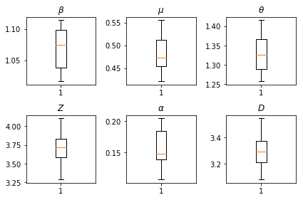
推断的结果。我们绘制所有全局参数的最大似然值,以显示它们在推断的 num_batches 独立运行中的差异。这与补充材料中的表 S1 对应。
fig, axs = plt.subplots(2, 3)
axs[0, 0].boxplot(best_parameters.documented_infectious_tx_rate,
                  whis=(2.5,97.5), sym='')
axs[0, 0].set_title(r'$\beta$')

axs[0, 1].boxplot(best_parameters.undocumented_infectious_tx_relative_rate,
                  whis=(2.5,97.5), sym='')
axs[0, 1].set_title(r'$\mu$')

axs[0, 2].boxplot(best_parameters.intercity_underreporting_factor,
                  whis=(2.5,97.5), sym='')
axs[0, 2].set_title(r'$\theta$')

axs[1, 0].boxplot(best_parameters.average_latency_period,
                  whis=(2.5,97.5), sym='')
axs[1, 0].set_title(r'$Z$')

axs[1, 1].boxplot(best_parameters.fraction_of_documented_infections,
                  whis=(2.5,97.5), sym='')
axs[1, 1].set_title(r'$\alpha$')

axs[1, 2].boxplot(best_parameters.average_infection_duration,
                  whis=(2.5,97.5), sym='')
axs[1, 2].set_title(r'$D$')
plt.tight_layout()