
| | |  צפה במקור ב-GitHub צפה במקור ב-GitHub | |
מדריך זה מראה כיצד רשת נוירונים קלאסית יכולה ללמוד לתקן שגיאות כיול קוויביט. הוא מציג את Cirq , מסגרת Python ליצירה, עריכה והפעלת מעגלי Noisy Intermediate Scale Quantum (NISQ), ומדגים כיצד Cirq מתממשק עם TensorFlow Quantum.
להכין
pip install tensorflow==2.7.0
התקן את TensorFlow Quantum:
pip install tensorflow-quantum
# Update package resources to account for version changes.
import importlib, pkg_resources
importlib.reload(pkg_resources)
<module 'pkg_resources' from '/tmpfs/src/tf_docs_env/lib/python3.7/site-packages/pkg_resources/__init__.py'>
כעת ייבא את TensorFlow ואת התלות של המודול:
import tensorflow as tf
import tensorflow_quantum as tfq

import cirq
import sympy
import numpy as np

# visualization tools
%matplotlib inline
import matplotlib.pyplot as plt
from cirq.contrib.svg import SVGCircuit
2022-02-04 12:27:31.677071: E tensorflow/stream_executor/cuda/cuda_driver.cc:271] failed call to cuInit: CUDA_ERROR_NO_DEVICE: no CUDA-capable device is detected
1. היסודות
1.1 Cirq ומעגלים קוונטיים עם פרמטרים
לפני שנחקור את TensorFlow Quantum (TFQ), בואו נסתכל על כמה יסודות של Cirq . Cirq היא ספריית Python עבור מחשוב קוונטי מגוגל. אתה משתמש בו כדי להגדיר מעגלים, כולל שערים סטטיים ופרמטרים.
Cirq משתמש בסמלי SymPy כדי לייצג פרמטרים חופשיים.
a, b = sympy.symbols('a b')
הקוד הבא יוצר מעגל שני קיוביטים באמצעות הפרמטרים שלך:
# Create two qubits
q0, q1 = cirq.GridQubit.rect(1, 2)

# Create a circuit on these qubits using the parameters you created above.
circuit = cirq.Circuit(
    cirq.rx(a).on(q0),
    cirq.ry(b).on(q1), cirq.CNOT(control=q0, target=q1))

SVGCircuit(circuit)
findfont: Font family ['Arial'] not found. Falling back to DejaVu Sans.

כדי להעריך מעגלים, אתה יכול להשתמש בממשק cirq.Simulator . אתה מחליף פרמטרים חופשיים במעגל עם מספרים ספציפיים על ידי העברת אובייקט cirq.ParamResolver . הקוד הבא מחשב את פלט וקטור המצב הגולמי של המעגל עם הפרמטרים שלך:
# Calculate a state vector with a=0.5 and b=-0.5.
resolver = cirq.ParamResolver({a: 0.5, b: -0.5})
output_state_vector = cirq.Simulator().simulate(circuit, resolver).final_state_vector
output_state_vector
array([ 0.9387913 +0.j        , -0.23971277+0.j        ,

        0.        +0.06120872j,  0.        -0.23971277j], dtype=complex64)
וקטורי מצב אינם נגישים ישירות מחוץ לסימולציה (שימו לב למספרים המרוכבים בפלט למעלה). כדי להיות מציאותי פיזית, עליך לציין מדידה, אשר ממירה וקטור מצב למספר ממשי שמחשבים קלאסיים יכולים להבין. Cirq מציין מדידות באמצעות שילובים של האופרטורים Pauli \(\hat{X}\), \(\hat{Y}\)ו- \(\hat{Z}\). כהמחשה, הקוד הבא מודד את \(\hat{Z}_0\) ו- \(\frac{1}{2}\hat{Z}_0 + \hat{X}_1\) בוקטור המצב שזה עתה סימלת:
z0 = cirq.Z(q0)

qubit_map={q0: 0, q1: 1}

z0.expectation_from_state_vector(output_state_vector, qubit_map).real
0.8775825500488281
z0x1 = 0.5 * z0 + cirq.X(q1)

z0x1.expectation_from_state_vector(output_state_vector, qubit_map).real
-0.04063427448272705
1.2 מעגלים קוונטיים כטנסורים
TensorFlow Quantum (TFQ) מספק tfq.convert_to_tensor , פונקציה הממירה אובייקטים של Cirq לטנזורים. זה מאפשר לך לשלוח אובייקטים של Cirq לשכבות הקוונטיות ולאופציות הקוונטיות שלנו. ניתן לקרוא לפונקציה ברשימות או מערכים של Cirq Circuits ו- Cirq Paulis:
# Rank 1 tensor containing 1 circuit.
circuit_tensor = tfq.convert_to_tensor([circuit])

print(circuit_tensor.shape)
print(circuit_tensor.dtype)
(1,)
<dtype: 'string'>
זה מקודד את אובייקטי tf.string tfq שפעולות tfq מפענחות לפי הצורך.
# Rank 1 tensor containing 2 Pauli operators.
pauli_tensor = tfq.convert_to_tensor([z0, z0x1])
pauli_tensor.shape
TensorShape([2])
1.3 הדמיית מעגל אצווה
TFQ מספק שיטות לחישוב ערכי ציפיות, דגימות ווקטורי מצב. לעת עתה, הבה נתמקד בערכי ציפיות .
הממשק ברמה הגבוהה ביותר לחישוב ערכי תוחלת הוא שכבת tfq.layers.Expectation , שהיא tf.keras.Layer . בצורתה הפשוטה ביותר, שכבה זו מקבילה להדמיית מעגל בעל פרמטרים על פני cirq.ParamResolvers רבים; עם זאת, TFQ מאפשר אצווה בעקבות סמנטיקה של TensorFlow, ומעגלים מדומים באמצעות קוד C++ יעיל.
צור אצווה של ערכים כדי להחליף את הפרמטרים a ו- b שלנו:
batch_vals = np.array(np.random.uniform(0, 2 * np.pi, (5, 2)), dtype=np.float32)
ביצוע מעגלים אצווה על ערכי פרמטרים ב-Cirq דורש לולאה:
cirq_results = []
cirq_simulator = cirq.Simulator()

for vals in batch_vals:
    resolver = cirq.ParamResolver({a: vals[0], b: vals[1]})
    final_state_vector = cirq_simulator.simulate(circuit, resolver).final_state_vector
    cirq_results.append(
        [z0.expectation_from_state_vector(final_state_vector, {
            q0: 0,
            q1: 1
        }).real])

print('cirq batch results: \n {}'.format(np.array(cirq_results)))
cirq batch results:
 [[-0.66652703]
 [ 0.49764055]
 [ 0.67326665]
 [-0.95549959]
 [-0.81297827]]
אותה פעולה מפושטת ב-TFQ:
tfq.layers.Expectation()(circuit,
                         symbol_names=[a, b],
                         symbol_values=batch_vals,
                         operators=z0)
<tf.Tensor: shape=(5, 1), dtype=float32, numpy=
array([[-0.666526  ],
       [ 0.49764216],
       [ 0.6732664 ],
       [-0.9554999 ],
       [-0.8129788 ]], dtype=float32)>
2. אופטימיזציה קוונטית-קלאסית היברידית
כעת, לאחר שראית את היסודות, בוא נשתמש ב- TensorFlow Quantum כדי לבנות רשת עצבית קוונטית-קלאסית היברידית . אתה תאמן רשת עצבית קלאסית לשלוט בקיוביט בודד. הבקרה תעבור אופטימיזציה להכנה נכונה של הקיוביט במצב 0 או 1 , תוך התגברות על שגיאת כיול שיטתית מדומה. איור זה מציג את הארכיטקטורה:
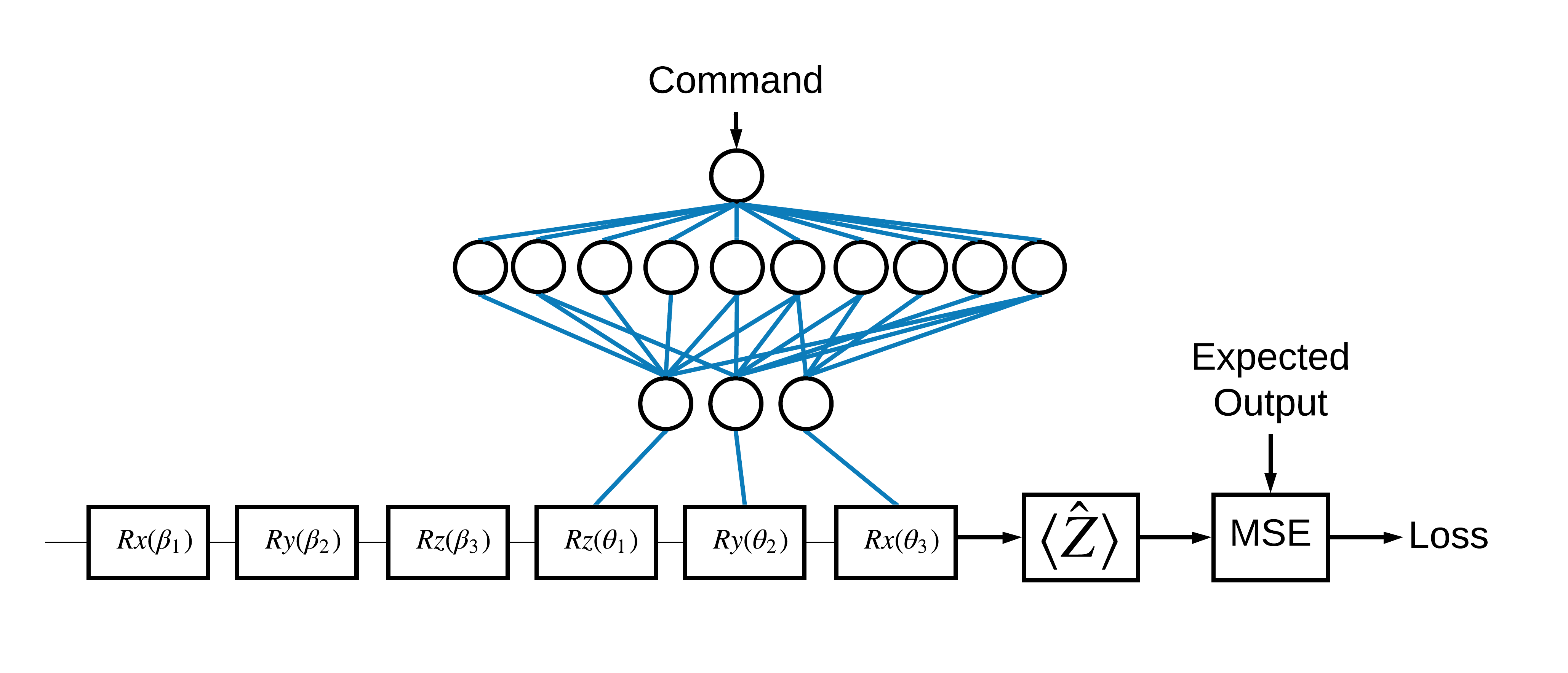
אפילו בלי רשת עצבית זו בעיה פשוטה לפתרון, אבל הנושא דומה לבעיות השליטה הקוונטיות האמיתיות שאתה עשוי לפתור באמצעות TFQ. הוא מדגים דוגמה מקצה לקצה של חישוב קוונטי-קלאסי באמצעות tfq.layers.ControlledPQC (Parametrized Quantum Circuit) בתוך שכבת tf.keras.Model .
לצורך יישום הדרכה זו, ארכיטקטורה זו מחולקת ל-3 חלקים:
- מעגל הקלט או מעגל נקודת הנתונים: שלושת השערים הראשונים \(R\) .
- המעגל המבוקר : שלושת השערים האחרים \(R\) .
- הבקר : הרשת העצבית הקלאסית קובעת את הפרמטרים של המעגל המבוקר.
2.1 הגדרת המעגל המבוקר
הגדר סיבוב סיביות בודד שניתן ללמוד, כפי שמצוין באיור למעלה. זה יתאים למעגל המבוקר שלנו.
# Parameters that the classical NN will feed values into.
control_params = sympy.symbols('theta_1 theta_2 theta_3')

# Create the parameterized circuit.
qubit = cirq.GridQubit(0, 0)
model_circuit = cirq.Circuit(
    cirq.rz(control_params[0])(qubit),
    cirq.ry(control_params[1])(qubit),
    cirq.rx(control_params[2])(qubit))

SVGCircuit(model_circuit)

2.2 הבקר
כעת הגדר את רשת הבקר:
# The classical neural network layers.
controller = tf.keras.Sequential([
    tf.keras.layers.Dense(10, activation='elu'),
    tf.keras.layers.Dense(3)
])
בהינתן אצווה של פקודות, הבקר מוציא אצווה של אותות בקרה עבור המעגל המבוקר.
הבקר מאותחל באופן אקראי ולכן הפלטים הללו אינם שימושיים, עדיין.
controller(tf.constant([[0.0],[1.0]])).numpy()
array([[0.        , 0.        , 0.        ],
       [0.5815686 , 0.21376055, 0.57181627]], dtype=float32)
2.3 חבר את הבקר למעגל
השתמש tfq כדי לחבר את הבקר למעגל המבוקר, כ- keras.Model יחיד.
עיין במדריך Keras Functional API למידע נוסף על סגנון זה של הגדרת המודל.
תחילה הגדר את התשומות למודל:
# This input is the simulated miscalibration that the model will learn to correct.
circuits_input = tf.keras.Input(shape=(),
                                # The circuit-tensor has dtype `tf.string`
                                dtype=tf.string,
                                name='circuits_input')

# Commands will be either `0` or `1`, specifying the state to set the qubit to.
commands_input = tf.keras.Input(shape=(1,),
                                dtype=tf.dtypes.float32,
                                name='commands_input')
לאחר מכן החל פעולות על אותן כניסות, כדי להגדיר את החישוב.
dense_2 = controller(commands_input)

# TFQ layer for classically controlled circuits.
expectation_layer = tfq.layers.ControlledPQC(model_circuit,
                                             # Observe Z
                                             operators = cirq.Z(qubit))
expectation = expectation_layer([circuits_input, dense_2])
כעת ארוז את החישוב הזה בתור tf.keras.Model :
# The full Keras model is built from our layers.
model = tf.keras.Model(inputs=[circuits_input, commands_input],
                       outputs=expectation)
ארכיטקטורת הרשת מסומנת על ידי העלילה של המודל שלהלן. השווה את עלילת המודל הזו לתרשים הארכיטקטורה כדי לוודא נכונות.
tf.keras.utils.plot_model(model, show_shapes=True, dpi=70)
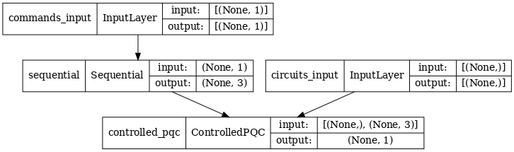
מודל זה לוקח שתי כניסות: הפקודות לבקר, ומעגל הקלט שאת הפלט שלו הבקר מנסה לתקן.
2.4 מערך הנתונים
המודל מנסה להוציא את ערך המדידה הנכון של \(\hat{Z}\) עבור כל פקודה. הפקודות והערכים הנכונים מוגדרים להלן.
# The command input values to the classical NN.
commands = np.array([[0], [1]], dtype=np.float32)

# The desired Z expectation value at output of quantum circuit.
expected_outputs = np.array([[1], [-1]], dtype=np.float32)
זה לא כל מערך ההדרכה למשימה זו. כל נקודת נתונים במערך הנתונים זקוקה גם למעגל קלט.
2.4 הגדרת מעגל קלט
מעגל הקלט להלן מגדיר את הכיול השגוי האקראי שהמודל ילמד לתקן.
random_rotations = np.random.uniform(0, 2 * np.pi, 3)
noisy_preparation = cirq.Circuit(
  cirq.rx(random_rotations[0])(qubit),
  cirq.ry(random_rotations[1])(qubit),
  cirq.rz(random_rotations[2])(qubit)
)
datapoint_circuits = tfq.convert_to_tensor([
  noisy_preparation
] * 2)  # Make two copied of this circuit
ישנם שני עותקים של המעגל, אחד עבור כל נקודת נתונים.
datapoint_circuits.shape
TensorShape([2])
2.5 הדרכה
עם הקלטות שהוגדרו תוכל להריץ בניסיון את מודל tfq .
model([datapoint_circuits, commands]).numpy()
array([[0.95853525],
       [0.6272128 ]], dtype=float32)
כעת הפעל תהליך הדרכה סטנדרטי כדי להתאים את הערכים הללו לכיוון ה- expected_outputs .
optimizer = tf.keras.optimizers.Adam(learning_rate=0.05)
loss = tf.keras.losses.MeanSquaredError()
model.compile(optimizer=optimizer, loss=loss)
history = model.fit(x=[datapoint_circuits, commands],
                    y=expected_outputs,
                    epochs=30,
                    verbose=0)
plt.plot(history.history['loss'])
plt.title("Learning to Control a Qubit")
plt.xlabel("Iterations")
plt.ylabel("Error in Control")
plt.show()
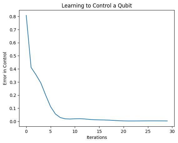
מהעלילה הזו ניתן לראות שהרשת העצבית למדה להתגבר על הכיול השגוי השיטתי.
2.6 אמת פלטים
כעת השתמש במודל המאומן, כדי לתקן את שגיאות כיול הקיוביט. עם Cirq:
def check_error(command_values, desired_values):
  """Based on the value in `command_value` see how well you could prepare
  the full circuit to have `desired_value` when taking expectation w.r.t. Z."""
  params_to_prepare_output = controller(command_values).numpy()
  full_circuit = noisy_preparation + model_circuit

  # Test how well you can prepare a state to get expectation the expectation
  # value in `desired_values`
  for index in [0, 1]:
    state = cirq_simulator.simulate(
        full_circuit,
        {s:v for (s,v) in zip(control_params, params_to_prepare_output[index])}
    ).final_state_vector
    expt = cirq.Z(qubit).expectation_from_state_vector(state, {qubit: 0}).real
    print(f'For a desired output (expectation) of {desired_values[index]} with'
          f' noisy preparation, the controller\nnetwork found the following '
          f'values for theta: {params_to_prepare_output[index]}\nWhich gives an'
          f' actual expectation of: {expt}\n')


check_error(commands, expected_outputs)
For a desired output (expectation) of [1.] with noisy preparation, the controller
network found the following values for theta: [-0.6788422   0.3395225  -0.59394693]
Which gives an actual expectation of: 0.9171845316886902

For a desired output (expectation) of [-1.] with noisy preparation, the controller
network found the following values for theta: [-5.203663   -0.29528576  3.2887425 ]
Which gives an actual expectation of: -0.9511058330535889
הערך של פונקציית ההפסד במהלך האימון מספק מושג גס עד כמה המודל לומד. ככל שההפסד נמוך יותר, ערכי הציפיות בתא שלמעלה קרובים יותר ל- desired_values . אם אתה לא כל כך מודאג מערכי הפרמטרים, אתה תמיד יכול לבדוק את הפלטים מלמעלה באמצעות tfq :
model([datapoint_circuits, commands])
<tf.Tensor: shape=(2, 1), dtype=float32, numpy=
array([[ 0.91718477],
       [-0.9511056 ]], dtype=float32)>
3 לימוד הכנת מצבים עצמיים של אופרטורים שונים
הבחירה של המצבים העצמיים \(\pm \hat{Z}\) המקבילים ל-1 ו-0 הייתה שרירותית. באותה מידה היית יכול לרצות ש-1 יתאים למצב \(+ \hat{Z}\) ו-0 יתאים למצב \(-\hat{X}\) . דרך אחת להשיג זאת היא על ידי ציון אופרטור מדידה שונה עבור כל פקודה, כפי שמצוין באיור שלהלן:

זה דורש שימוש ב- tfq.layers.Expectation . כעת הקלט שלך גדל לכלול שלושה אובייקטים: מעגל, פקודה ואופרטור. התפוקה היא עדיין ערך הצפי.
3.1 הגדרת דגם חדש
בואו נסתכל על המודל כדי לבצע משימה זו:
# Define inputs.
commands_input = tf.keras.layers.Input(shape=(1),
                                       dtype=tf.dtypes.float32,
                                       name='commands_input')
circuits_input = tf.keras.Input(shape=(),
                                # The circuit-tensor has dtype `tf.string`
                                dtype=tf.dtypes.string,
                                name='circuits_input')
operators_input = tf.keras.Input(shape=(1,),
                                 dtype=tf.dtypes.string,
                                 name='operators_input')
הנה רשת הבקר:
# Define classical NN.
controller = tf.keras.Sequential([
    tf.keras.layers.Dense(10, activation='elu'),
    tf.keras.layers.Dense(3)
])
שלב את המעגל והבקר ל- keras.Model יחידה. דגם באמצעות tfq :
dense_2 = controller(commands_input)

# Since you aren't using a PQC or ControlledPQC you must append
# your model circuit onto the datapoint circuit tensor manually.
full_circuit = tfq.layers.AddCircuit()(circuits_input, append=model_circuit)
expectation_output = tfq.layers.Expectation()(full_circuit,
                                              symbol_names=control_params,
                                              symbol_values=dense_2,
                                              operators=operators_input)

# Contruct your Keras model.
two_axis_control_model = tf.keras.Model(
    inputs=[circuits_input, commands_input, operators_input],
    outputs=[expectation_output])
3.2 מערך הנתונים
כעת תכלול גם את האופרטורים שברצונך למדוד עבור כל נקודת נתונים שאתה מספק עבור model_circuit :
# The operators to measure, for each command.
operator_data = tfq.convert_to_tensor([[cirq.X(qubit)], [cirq.Z(qubit)]])

# The command input values to the classical NN.
commands = np.array([[0], [1]], dtype=np.float32)

# The desired expectation value at output of quantum circuit.
expected_outputs = np.array([[1], [-1]], dtype=np.float32)
3.3 הדרכה
עכשיו, כשיש לך את הכניסות והיציאות החדשות שלך, אתה יכול להתאמן שוב באמצעות keras.
optimizer = tf.keras.optimizers.Adam(learning_rate=0.05)
loss = tf.keras.losses.MeanSquaredError()

two_axis_control_model.compile(optimizer=optimizer, loss=loss)

history = two_axis_control_model.fit(
    x=[datapoint_circuits, commands, operator_data],
    y=expected_outputs,
    epochs=30,
    verbose=1)
Epoch 1/30
1/1 [==============================] - 0s 320ms/step - loss: 2.4404
Epoch 2/30
1/1 [==============================] - 0s 3ms/step - loss: 1.8713
Epoch 3/30
1/1 [==============================] - 0s 3ms/step - loss: 1.1400
Epoch 4/30
1/1 [==============================] - 0s 3ms/step - loss: 0.5071
Epoch 5/30
1/1 [==============================] - 0s 3ms/step - loss: 0.1611
Epoch 6/30
1/1 [==============================] - 0s 3ms/step - loss: 0.0426
Epoch 7/30
1/1 [==============================] - 0s 3ms/step - loss: 0.0117
Epoch 8/30
1/1 [==============================] - 0s 3ms/step - loss: 0.0032
Epoch 9/30
1/1 [==============================] - 0s 2ms/step - loss: 0.0147
Epoch 10/30
1/1 [==============================] - 0s 3ms/step - loss: 0.0452
Epoch 11/30
1/1 [==============================] - 0s 3ms/step - loss: 0.0670
Epoch 12/30
1/1 [==============================] - 0s 3ms/step - loss: 0.0648
Epoch 13/30
1/1 [==============================] - 0s 3ms/step - loss: 0.0471
Epoch 14/30
1/1 [==============================] - 0s 3ms/step - loss: 0.0289
Epoch 15/30
1/1 [==============================] - 0s 3ms/step - loss: 0.0180
Epoch 16/30
1/1 [==============================] - 0s 3ms/step - loss: 0.0138
Epoch 17/30
1/1 [==============================] - 0s 2ms/step - loss: 0.0130
Epoch 18/30
1/1 [==============================] - 0s 3ms/step - loss: 0.0137
Epoch 19/30
1/1 [==============================] - 0s 3ms/step - loss: 0.0148
Epoch 20/30
1/1 [==============================] - 0s 3ms/step - loss: 0.0156
Epoch 21/30
1/1 [==============================] - 0s 3ms/step - loss: 0.0157
Epoch 22/30
1/1 [==============================] - 0s 3ms/step - loss: 0.0149
Epoch 23/30
1/1 [==============================] - 0s 3ms/step - loss: 0.0135
Epoch 24/30
1/1 [==============================] - 0s 3ms/step - loss: 0.0119
Epoch 25/30
1/1 [==============================] - 0s 3ms/step - loss: 0.0100
Epoch 26/30
1/1 [==============================] - 0s 3ms/step - loss: 0.0082
Epoch 27/30
1/1 [==============================] - 0s 3ms/step - loss: 0.0064
Epoch 28/30
1/1 [==============================] - 0s 3ms/step - loss: 0.0047
Epoch 29/30
1/1 [==============================] - 0s 3ms/step - loss: 0.0034
Epoch 30/30
1/1 [==============================] - 0s 3ms/step - loss: 0.0024
plt.plot(history.history['loss'])
plt.title("Learning to Control a Qubit")
plt.xlabel("Iterations")
plt.ylabel("Error in Control")
plt.show()
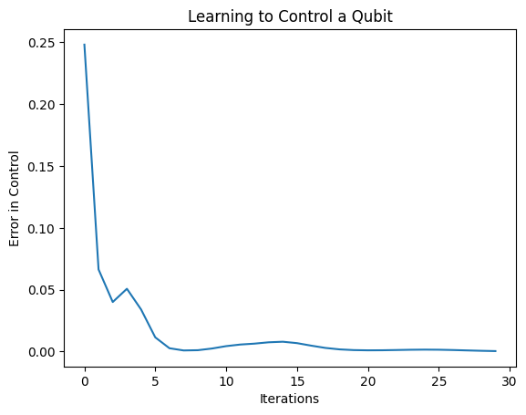
פונקציית ההפסד ירדה לאפס.
controller זמין כדגם עצמאי. התקשר לבקר, ובדקו את תגובתו לכל אות פקודה. תידרש קצת עבודה כדי להשוות נכון את הפלטים הללו לתוכן של random_rotations .
controller.predict(np.array([0,1]))
array([[3.6335812 , 1.8470774 , 0.71675825],
       [5.3085413 , 0.08116499, 2.8337662 ]], dtype=float32)