
 GitHub でソースを表示 GitHub でソースを表示 |
概要
TensorFlow Image Summary API を使用すると、テンソルと任意の画像のログと TensorBoard での表示を簡単に行えるようになります。入力データをサンプリングして調べる場合や、レイヤーの重みや生成されたテンソルを視覚化する場合に非常に有用です。また、診断データを画像としてログすることもできるため、モデル開発時に役立ちます。
このチュートリアルでは、Image Summary API を使用してテンソルを画像として視覚化する方法を学習します。また、任意の画像からテンソルに変換し、それを TensorBoard で視覚化する方法も学習します。モデルのパフォーマンスを理解しやすいように、Image Summary を使用する単純な実際の例を使って作業します。
セットアップ
try:
  # %tensorflow_version only exists in Colab.
  %tensorflow_version 2.x
except Exception:
  pass

# Load the TensorBoard notebook extension.
%load_ext tensorboard
TensorFlow 2.x selected.
from datetime import datetime
import io
import itertools
from packaging import version

import tensorflow as tf
from tensorflow import keras

import matplotlib.pyplot as plt
import numpy as np
import sklearn.metrics

print("TensorFlow version: ", tf.__version__)
assert version.parse(tf.__version__).release[0] >= 2, \
    "This notebook requires TensorFlow 2.0 or above."
TensorFlow version: 2.2
Fashion-MNIST データセットをダウンロードする
Fashion-MNIST データセットの画像を分類する、簡単なニューラルネットワークを構築しましょう。このデータセットには、ファッション製品に関する 70,000 個の 28x28 グレースケール画像が含まれています。7,000 個の画像を含むカテゴリが全 10 個あります。
まず、データをダウンロードします。
# Download the data. The data is already divided into train and test.
# The labels are integers representing classes.
fashion_mnist = keras.datasets.fashion_mnist
(train_images, train_labels), (test_images, test_labels) = \
    fashion_mnist.load_data()

# Names of the integer classes, i.e., 0 -> T-short/top, 1 -> Trouser, etc.
class_names = ['T-shirt/top', 'Trouser', 'Pullover', 'Dress', 'Coat',
    'Sandal', 'Shirt', 'Sneaker', 'Bag', 'Ankle boot']
Downloading data from https://storage.googleapis.com/tensorflow/tf-keras-datasets/train-labels-idx1-ubyte.gz
32768/29515 [=================================] - 0s 0us/step
Downloading data from https://storage.googleapis.com/tensorflow/tf-keras-datasets/train-images-idx3-ubyte.gz
26427392/26421880 [==============================] - 0s 0us/step
Downloading data from https://storage.googleapis.com/tensorflow/tf-keras-datasets/t10k-labels-idx1-ubyte.gz
8192/5148 [===============================================] - 0s 0us/step
Downloading data from https://storage.googleapis.com/tensorflow/tf-keras-datasets/t10k-images-idx3-ubyte.gz
4423680/4422102 [==============================] - 0s 0us/step
1 つの画像を視覚化する
Image Summary API の動作を理解するために、トレーニングセットの最初のトレーニング画像を単純に TensorBoard ログすることにします。
これを行う前に、トレーニングデータの形状を調べてみましょう。
print("Shape: ", train_images[0].shape)
print("Label: ", train_labels[0], "->", class_names[train_labels[0]])
Shape:  (28, 28)
Label:  9 -> Ankle boot
データセットの各画像の形状は、高さと幅を表す形状 (28, 28) の階数 2 テンソルです。
しかし、tf.summary.image() には (batch_size, height, width, channels) を含む階数 4 のテンソルが必要であるため、形状を変更する必要があります。
1 つの画像のみをログしているため、batch_size は 1 となります。画像はグレースケールであるため、channels を 1 とします。
# Reshape the image for the Summary API.
img = np.reshape(train_images[0], (-1, 28, 28, 1))
これで画像をログし、TensorBoard で表示する準備が整いました。
# Clear out any prior log data.
!rm -rf logs

# Sets up a timestamped log directory.
logdir = "logs/train_data/" + datetime.now().strftime("%Y%m%d-%H%M%S")
# Creates a file writer for the log directory.
file_writer = tf.summary.create_file_writer(logdir)

# Using the file writer, log the reshaped image.
with file_writer.as_default():
  tf.summary.image("Training data", img, step=0)
では、TensorBoard を使用して画像を調べてみましょう。UI が読み込まれるまで数秒待ちます。
%tensorboard --logdir logs/train_data

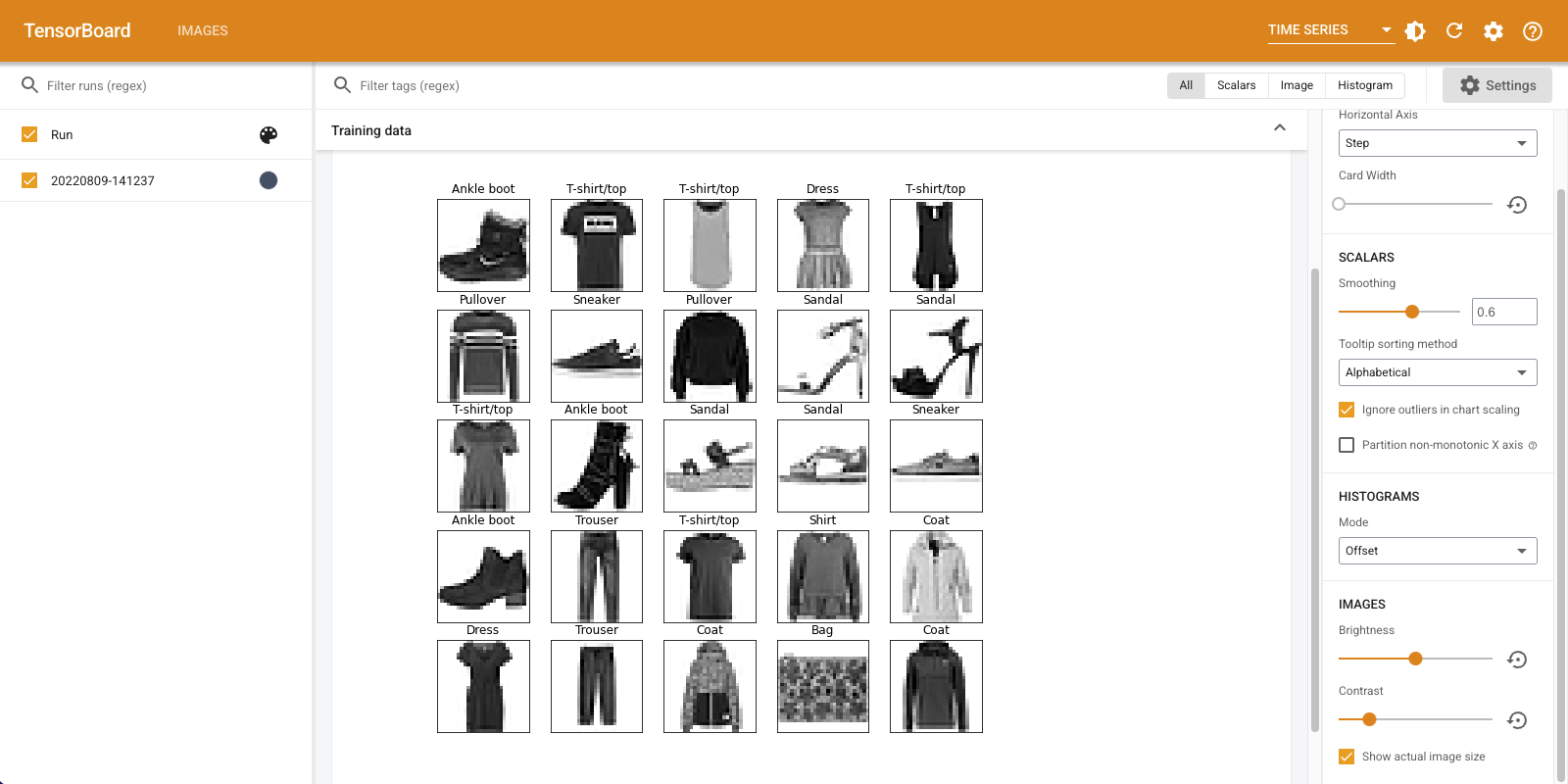
「Time Series」ダッシュボードに、今ログした画像が表示されます。「ankle boot(アンクルブーツ)」です。
画像は見やすいようにデフォルトのサイズに調整されています。スケーリングなしの元の画像を表示する場合は、右側の「Settings」パネル下の「Show actual image size」のチェックをオンにしてください。
明るさやコントラストのスライダを動かして、画像のピクセルにどのような影響があるかを確認します。
複数の画像を視覚化する
1 つのテンソルをログするのはうまくいきましたが、複数のトレーニングサンプルをログする場合はどうすればよいのでしょうか。
データを tf.summary.image() に渡す際に、ログする画像数を指定するだけです。
with file_writer.as_default():
  # Don't forget to reshape.
  images = np.reshape(train_images[0:25], (-1, 28, 28, 1))
  tf.summary.image("25 training data examples", images, max_outputs=25, step=0)

%tensorboard --logdir logs/train_data

任意の画像をログする
matplotlib が生成する画像など、テンソルでない画像を視覚化する場合はどうでしょうか。
プロットをテンソルに変換するボイラープレートコードのようなものが必要となりますが、それを通過すればこの問題はクリアです。
次のコードでは、matplotlib の subplot() 関数を使用して最初の 25 個の画像を適切なグリッドとしてログし、その後で、そのグリッドを TensorBoard で表示します。
# Clear out prior logging data.
!rm -rf logs/plots

logdir = "logs/plots/" + datetime.now().strftime("%Y%m%d-%H%M%S")
file_writer = tf.summary.create_file_writer(logdir)

def plot_to_image(figure):
  """Converts the matplotlib plot specified by 'figure' to a PNG image and
  returns it. The supplied figure is closed and inaccessible after this call."""
  # Save the plot to a PNG in memory.
  buf = io.BytesIO()
  plt.savefig(buf, format='png')
  # Closing the figure prevents it from being displayed directly inside
  # the notebook.
  plt.close(figure)
  buf.seek(0)
  # Convert PNG buffer to TF image
  image = tf.image.decode_png(buf.getvalue(), channels=4)
  # Add the batch dimension
  image = tf.expand_dims(image, 0)
  return image

def image_grid():
  """Return a 5x5 grid of the MNIST images as a matplotlib figure."""
  # Create a figure to contain the plot.
  figure = plt.figure(figsize=(10,10))
  for i in range(25):
    # Start next subplot.
    plt.subplot(5, 5, i + 1, title=class_names[train_labels[i]])
    plt.xticks([])
    plt.yticks([])
    plt.grid(False)
    plt.imshow(train_images[i], cmap=plt.cm.binary)

  return figure

# Prepare the plot
figure = image_grid()
# Convert to image and log
with file_writer.as_default():
  tf.summary.image("Training data", plot_to_image(figure), step=0)

%tensorboard --logdir logs/plots
画像分類器を構築する
綺麗な写真をプロットするためではなく、機械学習を行うためにこのチュートリアルを行っているわけですから、この作業を実際の例に適用してみましょう。
画像の要約を使用して、Fashion-MNIST データセットの簡単な分類器をトレーニングしながらモデルがどれほどうまく機能しているかを把握することにします。
まず、非常に単純なモデルを作成してコンパイルします。オプティマイザと損失関数をセットアップしましょう。コンパイルのステップでは分類器の精度も合わせてログすることを指定します。
model = keras.models.Sequential([
    keras.layers.Flatten(input_shape=(28, 28)),
    keras.layers.Dense(32, activation='relu'),
    keras.layers.Dense(10, activation='softmax')
])

model.compile(
    optimizer='adam',
    loss='sparse_categorical_crossentropy',
    metrics=['accuracy']
)
分類器をトレーニングする際、混同行列を見ると役に立ちます。混同行列では、分類器がテストデータどどのように実行しているかを詳しく知ることができます。
混同行列を計算する関数を定義しましょう。Scikit-learn 関数を使えば簡単にこれを行え、その上で、matplotlib を使ってプロットすることができます。
def plot_confusion_matrix(cm, class_names):
  """
  Returns a matplotlib figure containing the plotted confusion matrix.

  Args:
    cm (array, shape = [n, n]): a confusion matrix of integer classes
    class_names (array, shape = [n]): String names of the integer classes
  """
  figure = plt.figure(figsize=(8, 8))
  plt.imshow(cm, interpolation='nearest', cmap=plt.cm.Blues)
  plt.title("Confusion matrix")
  plt.colorbar()
  tick_marks = np.arange(len(class_names))
  plt.xticks(tick_marks, class_names, rotation=45)
  plt.yticks(tick_marks, class_names)

  # Compute the labels from the normalized confusion matrix.
  labels = np.around(cm.astype('float') / cm.sum(axis=1)[:, np.newaxis], decimals=2)

  # Use white text if squares are dark; otherwise black.
  threshold = cm.max() / 2.
  for i, j in itertools.product(range(cm.shape[0]), range(cm.shape[1])):
    color = "white" if cm[i, j] > threshold else "black"
    plt.text(j, i, labels[i, j], horizontalalignment="center", color=color)

  plt.tight_layout()
  plt.ylabel('True label')
  plt.xlabel('Predicted label')
  return figure
これで、分類器をトレーニングしながら混同行列を定期的にログする準備が整いました。
ここでは、次の項目を行います。
- 基本的なメトリックをログする Keras TensorBoard コールバックを作成する
- エポックが終了するたびに混同行列をログする Keras LambdaCallback を作成する
- 両方のコールバックが渡されるようにし、Model.fit() を使ってモデルをトレーニングする
トレーニングが進むにつれ、下にスクロールして TensorBoard の起動を確認します。
# Clear out prior logging data.
!rm -rf logs/image

logdir = "logs/image/" + datetime.now().strftime("%Y%m%d-%H%M%S")
# Define the basic TensorBoard callback.
tensorboard_callback = keras.callbacks.TensorBoard(log_dir=logdir)
file_writer_cm = tf.summary.create_file_writer(logdir + '/cm')
def log_confusion_matrix(epoch, logs):
  # Use the model to predict the values from the validation dataset.
  test_pred_raw = model.predict(test_images)
  test_pred = np.argmax(test_pred_raw, axis=1)

  # Calculate the confusion matrix.
  cm = sklearn.metrics.confusion_matrix(test_labels, test_pred)
  # Log the confusion matrix as an image summary.
  figure = plot_confusion_matrix(cm, class_names=class_names)
  cm_image = plot_to_image(figure)

  # Log the confusion matrix as an image summary.
  with file_writer_cm.as_default():
    tf.summary.image("epoch_confusion_matrix", cm_image, step=epoch)

# Define the per-epoch callback.
cm_callback = keras.callbacks.LambdaCallback(on_epoch_end=log_confusion_matrix)
# Start TensorBoard.
%tensorboard --logdir logs/image

# Train the classifier.
model.fit(
    train_images,
    train_labels,
    epochs=5,
    verbose=0, # Suppress chatty output
    callbacks=[tensorboard_callback, cm_callback],
    validation_data=(test_images, test_labels),
)
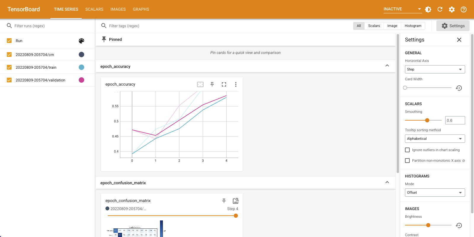
トレーニングと検証の両方のセットで、精度が上昇して言えるのがわかります。これは良い兆しではありますが、データの特定のサブセットで実行しているモデルはどうなっているでしょうか。
「Time Series」ダッシュボードを下にスクロールし、ログした混同行列を可視化してみましょう。「Settings」パネルの下にある「Show actual image size」をオンにして、混同行列をフルサイズで表示します。
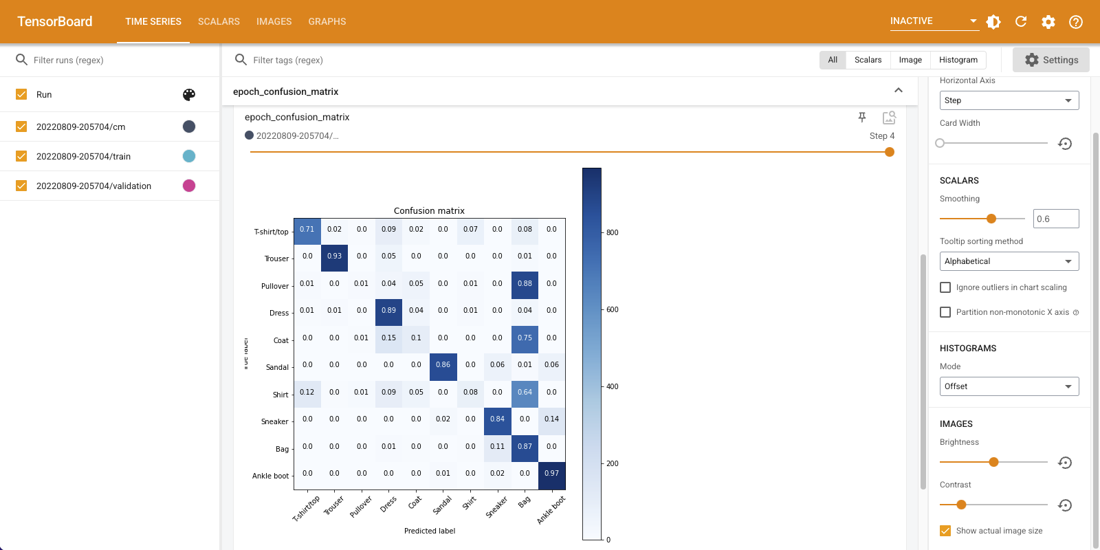
デフォルトでは、このダッシュボードには最後にログされたステップまたはエポックの画像要約が表示されます。スライダーを使用して早期の混同行列を表示します。トレーニングが進むにつれ、行列が大きく変化しているのがわかります。暗めのマスが斜めに連なり、ほかの行列は 0 に近くマスの色も白くなっています。つまり、トレーニングが進むにつれ、分類器が改善しているということです。よくできました!
混同行列は、この単純なモデルにいくつかの問題があることを示しています。うまく進んではいるものの、シャツ、Tシャツ、プルオーバーが混同されているため、モデルの改善が必要です。
関心のある方は、このモデルを畳み込みネットワーク(CNN)で改善してみてください。