
|
|
|
 View on GitHub View on GitHub
|
|
In this colab, you will learn how to inspect and create the structure of a model directly. We assume you are familiar with the concepts introduced in the beginner and intermediate colabs.
In this colab, you will:
Train a Random Forest model and access its structure programmatically.
Create a Random Forest model by hand and use it as a classical model.
Setup
# Install TensorFlow Decision Forests.pip install tensorflow_decision_forests# Use wurlitzer to show the training logs.pip install wurlitzer
import os
# Keep using Keras 2
os.environ['TF_USE_LEGACY_KERAS'] = '1'

import tensorflow_decision_forests as tfdf

import numpy as np
import pandas as pd
import tensorflow as tf
import tf_keras
import matplotlib.pyplot as plt
import math
import collections
The hidden code cell limits the output height in colab.
from IPython.core.magic import register_line_magic
from IPython.display import Javascript
from IPython.display import display as ipy_display

# Some of the model training logs can cover the full
# screen if not compressed to a smaller viewport.
# This magic allows setting a max height for a cell.
@register_line_magic
def set_cell_height(size):
  ipy_display(
      Javascript("google.colab.output.setIframeHeight(0, true, {maxHeight: " +
                 str(size) + "})"))
Train a simple Random Forest
We train a Random Forest like in the beginner colab:
# Download the dataset
!wget -q https://storage.googleapis.com/download.tensorflow.org/data/palmer_penguins/penguins.csv -O /tmp/penguins.csv

# Load a dataset into a Pandas Dataframe.
dataset_df = pd.read_csv("/tmp/penguins.csv")

# Show the first three examples.
print(dataset_df.head(3))

# Convert the pandas dataframe into a tf dataset.
dataset_tf = tfdf.keras.pd_dataframe_to_tf_dataset(dataset_df, label="species")

# Train the Random Forest
model = tfdf.keras.RandomForestModel(compute_oob_variable_importances=True)
model.fit(x=dataset_tf)
species     island  bill_length_mm  bill_depth_mm  flipper_length_mm  \
0  Adelie  Torgersen            39.1           18.7              181.0
1  Adelie  Torgersen            39.5           17.4              186.0
2  Adelie  Torgersen            40.3           18.0              195.0

   body_mass_g     sex  year
0       3750.0    male  2007
1       3800.0  female  2007
2       3250.0  female  2007
Warning: The `num_threads` constructor argument is not set and the number of CPU is os.cpu_count()=32 > 32. Setting num_threads to 32. Set num_threads manually to use more than 32 cpus.
WARNING:absl:The `num_threads` constructor argument is not set and the number of CPU is os.cpu_count()=32 > 32. Setting num_threads to 32. Set num_threads manually to use more than 32 cpus.
Use /tmpfs/tmp/tmp71p_zbfn as temporary training directory
Reading training dataset...
Training dataset read in 0:00:03.783666. Found 344 examples.
Training model...
Model trained in 0:00:00.091364
Compiling model...
[INFO 24-03-15 11:30:58.6002 UTC kernel.cc:1233] Loading model from path /tmpfs/tmp/tmp71p_zbfn/model/ with prefix 79891677e19b4595
[INFO 24-03-15 11:30:58.6165 UTC decision_forest.cc:734] Model loaded with 300 root(s), 5080 node(s), and 7 input feature(s).
[INFO 24-03-15 11:30:58.6166 UTC abstract_model.cc:1344] Engine "RandomForestGeneric" built
[INFO 24-03-15 11:30:58.6166 UTC kernel.cc:1061] Use fast generic engine
Model compiled.
<tf_keras.src.callbacks.History at 0x7f6cf8913f40>
Note the compute_oob_variable_importances=True
hyper-parameter in the model constructor. This option computes the Out-of-bag (OOB)
variable importance during training. This is a popular
permutation variable importance for Random Forest models.
Computing the OOB Variable importance does not impact the final model, it will slow the training on large datasets.
Check the model summary:
%set_cell_height 300

model.summary()
<IPython.core.display.Javascript object>
Model: "random_forest_model"
_________________________________________________________________
 Layer (type)                Output Shape              Param #
=================================================================
=================================================================
Total params: 1 (1.00 Byte)
Trainable params: 0 (0.00 Byte)
Non-trainable params: 1 (1.00 Byte)
_________________________________________________________________
Type: "RANDOM_FOREST"
Task: CLASSIFICATION
Label: "__LABEL"

Input Features (7):
    bill_depth_mm
    bill_length_mm
    body_mass_g
    flipper_length_mm
    island
    sex
    year

No weights

Variable Importance: INV_MEAN_MIN_DEPTH:

    1. "flipper_length_mm"  0.440513 ################
    2.    "bill_length_mm"  0.438028 ###############
    3.     "bill_depth_mm"  0.299751 #####
    4.            "island"  0.295079 #####
    5.       "body_mass_g"  0.256534 ##
    6.               "sex"  0.225708
    7.              "year"  0.224020

Variable Importance: MEAN_DECREASE_IN_ACCURACY:

    1.    "bill_length_mm"  0.151163 ################
    2.            "island"  0.008721 #
    3.     "bill_depth_mm"  0.000000
    4.       "body_mass_g"  0.000000
    5.               "sex"  0.000000
    6.              "year"  0.000000
    7. "flipper_length_mm" -0.002907

Variable Importance: MEAN_DECREASE_IN_AP_1_VS_OTHERS:

    1.    "bill_length_mm"  0.083305 ################
    2.            "island"  0.007664 #
    3. "flipper_length_mm"  0.003400
    4.     "bill_depth_mm"  0.002741
    5.       "body_mass_g"  0.000722
    6.               "sex"  0.000644
    7.              "year"  0.000000

Variable Importance: MEAN_DECREASE_IN_AP_2_VS_OTHERS:

    1.    "bill_length_mm"  0.508510 ################
    2.            "island"  0.023487
    3.     "bill_depth_mm"  0.007744
    4. "flipper_length_mm"  0.006008
    5.       "body_mass_g"  0.003017
    6.               "sex"  0.001537
    7.              "year" -0.000245

Variable Importance: MEAN_DECREASE_IN_AP_3_VS_OTHERS:

    1.            "island"  0.002192 ################
    2.    "bill_length_mm"  0.001572 ############
    3.     "bill_depth_mm"  0.000497 #######
    4.               "sex"  0.000000 ####
    5.              "year"  0.000000 ####
    6.       "body_mass_g" -0.000053 ####
    7. "flipper_length_mm" -0.000890

Variable Importance: MEAN_DECREASE_IN_AUC_1_VS_OTHERS:

    1.    "bill_length_mm"  0.071306 ################
    2.            "island"  0.007299 #
    3. "flipper_length_mm"  0.004506 #
    4.     "bill_depth_mm"  0.002124
    5.       "body_mass_g"  0.000548
    6.               "sex"  0.000480
    7.              "year"  0.000000

Variable Importance: MEAN_DECREASE_IN_AUC_2_VS_OTHERS:

    1.    "bill_length_mm"  0.108642 ################
    2.            "island"  0.014493 ##
    3.     "bill_depth_mm"  0.007406 #
    4. "flipper_length_mm"  0.005195
    5.       "body_mass_g"  0.001012
    6.               "sex"  0.000480
    7.              "year" -0.000053

Variable Importance: MEAN_DECREASE_IN_AUC_3_VS_OTHERS:

    1.            "island"  0.002126 ################
    2.    "bill_length_mm"  0.001393 ###########
    3.     "bill_depth_mm"  0.000293 #####
    4.               "sex"  0.000000 ###
    5.              "year"  0.000000 ###
    6.       "body_mass_g" -0.000037 ###
    7. "flipper_length_mm" -0.000550

Variable Importance: MEAN_DECREASE_IN_PRAUC_1_VS_OTHERS:

    1.    "bill_length_mm"  0.083122 ################
    2.            "island"  0.010887 ##
    3. "flipper_length_mm"  0.003425
    4.     "bill_depth_mm"  0.002731
    5.       "body_mass_g"  0.000719
    6.               "sex"  0.000641
    7.              "year"  0.000000

Variable Importance: MEAN_DECREASE_IN_PRAUC_2_VS_OTHERS:

    1.    "bill_length_mm"  0.497611 ################
    2.            "island"  0.024045
    3.     "bill_depth_mm"  0.007734
    4. "flipper_length_mm"  0.006017
    5.       "body_mass_g"  0.003000
    6.               "sex"  0.001528
    7.              "year" -0.000243

Variable Importance: MEAN_DECREASE_IN_PRAUC_3_VS_OTHERS:

    1.            "island"  0.002187 ################
    2.    "bill_length_mm"  0.001568 ############
    3.     "bill_depth_mm"  0.000495 #######
    4.               "sex"  0.000000 ####
    5.              "year"  0.000000 ####
    6.       "body_mass_g" -0.000053 ####
    7. "flipper_length_mm" -0.000886

Variable Importance: NUM_AS_ROOT:

    1. "flipper_length_mm" 157.000000 ################
    2.    "bill_length_mm" 76.000000 #######
    3.     "bill_depth_mm" 52.000000 #####
    4.            "island" 12.000000
    5.       "body_mass_g"  3.000000

Variable Importance: NUM_NODES:

    1.    "bill_length_mm" 778.000000 ################
    2.     "bill_depth_mm" 463.000000 #########
    3. "flipper_length_mm" 414.000000 ########
    4.            "island" 342.000000 ######
    5.       "body_mass_g" 338.000000 ######
    6.               "sex" 36.000000
    7.              "year" 19.000000

Variable Importance: SUM_SCORE:

    1.    "bill_length_mm" 36515.793787 ################
    2. "flipper_length_mm" 35120.434174 ###############
    3.            "island" 14669.408395 ######
    4.     "bill_depth_mm" 14515.446617 ######
    5.       "body_mass_g" 3485.330881 #
    6.               "sex" 354.201073
    7.              "year" 49.737758


Winner takes all: true
Out-of-bag evaluation: accuracy:0.976744 logloss:0.068949
Number of trees: 300
Total number of nodes: 5080

Number of nodes by tree:
Count: 300 Average: 16.9333 StdDev: 3.10197
Min: 11 Max: 31 Ignored: 0
----------------------------------------------
[ 11, 12)  6   2.00%   2.00% #
[ 12, 13)  0   0.00%   2.00%
[ 13, 14) 46  15.33%  17.33% #####
[ 14, 15)  0   0.00%  17.33%
[ 15, 16) 70  23.33%  40.67% ########
[ 16, 17)  0   0.00%  40.67%
[ 17, 18) 84  28.00%  68.67% ##########
[ 18, 19)  0   0.00%  68.67%
[ 19, 20) 46  15.33%  84.00% #####
[ 20, 21)  0   0.00%  84.00%
[ 21, 22) 30  10.00%  94.00% ####
[ 22, 23)  0   0.00%  94.00%
[ 23, 24) 13   4.33%  98.33% ##
[ 24, 25)  0   0.00%  98.33%
[ 25, 26)  2   0.67%  99.00%
[ 26, 27)  0   0.00%  99.00%
[ 27, 28)  2   0.67%  99.67%
[ 28, 29)  0   0.00%  99.67%
[ 29, 30)  0   0.00%  99.67%
[ 30, 31]  1   0.33% 100.00%

Depth by leafs:
Count: 2690 Average: 3.53271 StdDev: 1.06789
Min: 2 Max: 7 Ignored: 0
----------------------------------------------
[ 2, 3) 545  20.26%  20.26% ######
[ 3, 4) 747  27.77%  48.03% ########
[ 4, 5) 888  33.01%  81.04% ##########
[ 5, 6) 444  16.51%  97.55% #####
[ 6, 7)  62   2.30%  99.85% #
[ 7, 7]   4   0.15% 100.00%

Number of training obs by leaf:
Count: 2690 Average: 38.3643 StdDev: 44.8651
Min: 5 Max: 155 Ignored: 0
----------------------------------------------
[   5,  12) 1474  54.80%  54.80% ##########
[  12,  20)  124   4.61%  59.41% #
[  20,  27)   48   1.78%  61.19%
[  27,  35)   74   2.75%  63.94% #
[  35,  42)   58   2.16%  66.10%
[  42,  50)   85   3.16%  69.26% #
[  50,  57)   96   3.57%  72.83% #
[  57,  65)   87   3.23%  76.06% #
[  65,  72)   49   1.82%  77.88%
[  72,  80)   23   0.86%  78.74%
[  80,  88)   30   1.12%  79.85%
[  88,  95)   23   0.86%  80.71%
[  95, 103)   42   1.56%  82.27%
[ 103, 110)   62   2.30%  84.57%
[ 110, 118)  115   4.28%  88.85% #
[ 118, 125)  115   4.28%  93.12% #
[ 125, 133)   98   3.64%  96.77% #
[ 133, 140)   49   1.82%  98.59%
[ 140, 148)   31   1.15%  99.74%
[ 148, 155]    7   0.26% 100.00%

Attribute in nodes:
    778 : bill_length_mm [NUMERICAL]
    463 : bill_depth_mm [NUMERICAL]
    414 : flipper_length_mm [NUMERICAL]
    342 : island [CATEGORICAL]
    338 : body_mass_g [NUMERICAL]
    36 : sex [CATEGORICAL]
    19 : year [NUMERICAL]

Attribute in nodes with depth <= 0:
    157 : flipper_length_mm [NUMERICAL]
    76 : bill_length_mm [NUMERICAL]
    52 : bill_depth_mm [NUMERICAL]
    12 : island [CATEGORICAL]
    3 : body_mass_g [NUMERICAL]

Attribute in nodes with depth <= 1:
    250 : bill_length_mm [NUMERICAL]
    244 : flipper_length_mm [NUMERICAL]
    183 : bill_depth_mm [NUMERICAL]
    170 : island [CATEGORICAL]
    53 : body_mass_g [NUMERICAL]

Attribute in nodes with depth <= 2:
    462 : bill_length_mm [NUMERICAL]
    320 : flipper_length_mm [NUMERICAL]
    310 : bill_depth_mm [NUMERICAL]
    287 : island [CATEGORICAL]
    162 : body_mass_g [NUMERICAL]
    9 : sex [CATEGORICAL]
    5 : year [NUMERICAL]

Attribute in nodes with depth <= 3:
    669 : bill_length_mm [NUMERICAL]
    410 : bill_depth_mm [NUMERICAL]
    383 : flipper_length_mm [NUMERICAL]
    328 : island [CATEGORICAL]
    286 : body_mass_g [NUMERICAL]
    32 : sex [CATEGORICAL]
    10 : year [NUMERICAL]

Attribute in nodes with depth <= 5:
    778 : bill_length_mm [NUMERICAL]
    462 : bill_depth_mm [NUMERICAL]
    413 : flipper_length_mm [NUMERICAL]
    342 : island [CATEGORICAL]
    338 : body_mass_g [NUMERICAL]
    36 : sex [CATEGORICAL]
    19 : year [NUMERICAL]

Condition type in nodes:
    2012 : HigherCondition
    378 : ContainsBitmapCondition
Condition type in nodes with depth <= 0:
    288 : HigherCondition
    12 : ContainsBitmapCondition
Condition type in nodes with depth <= 1:
    730 : HigherCondition
    170 : ContainsBitmapCondition
Condition type in nodes with depth <= 2:
    1259 : HigherCondition
    296 : ContainsBitmapCondition
Condition type in nodes with depth <= 3:
    1758 : HigherCondition
    360 : ContainsBitmapCondition
Condition type in nodes with depth <= 5:
    2010 : HigherCondition
    378 : ContainsBitmapCondition
Node format: NOT_SET

Training OOB:
    trees: 1, Out-of-bag evaluation: accuracy:0.964286 logloss:1.28727
    trees: 11, Out-of-bag evaluation: accuracy:0.951128 logloss:1.09857
    trees: 27, Out-of-bag evaluation: accuracy:0.959877 logloss:0.703445
    trees: 39, Out-of-bag evaluation: accuracy:0.961765 logloss:0.480034
    trees: 49, Out-of-bag evaluation: accuracy:0.965116 logloss:0.181201
    trees: 60, Out-of-bag evaluation: accuracy:0.973837 logloss:0.179433
    trees: 71, Out-of-bag evaluation: accuracy:0.973837 logloss:0.174384
    trees: 95, Out-of-bag evaluation: accuracy:0.976744 logloss:0.171732
    trees: 105, Out-of-bag evaluation: accuracy:0.976744 logloss:0.1714
    trees: 116, Out-of-bag evaluation: accuracy:0.976744 logloss:0.0764072
    trees: 131, Out-of-bag evaluation: accuracy:0.976744 logloss:0.0742712
    trees: 147, Out-of-bag evaluation: accuracy:0.976744 logloss:0.0737618
    trees: 158, Out-of-bag evaluation: accuracy:0.976744 logloss:0.0724368
    trees: 169, Out-of-bag evaluation: accuracy:0.976744 logloss:0.0710161
    trees: 180, Out-of-bag evaluation: accuracy:0.976744 logloss:0.0711254
    trees: 193, Out-of-bag evaluation: accuracy:0.976744 logloss:0.0691271
    trees: 204, Out-of-bag evaluation: accuracy:0.976744 logloss:0.0693627
    trees: 220, Out-of-bag evaluation: accuracy:0.976744 logloss:0.0687925
    trees: 232, Out-of-bag evaluation: accuracy:0.976744 logloss:0.0697578
    trees: 242, Out-of-bag evaluation: accuracy:0.976744 logloss:0.069291
    trees: 255, Out-of-bag evaluation: accuracy:0.976744 logloss:0.0693713
    trees: 268, Out-of-bag evaluation: accuracy:0.976744 logloss:0.0689708
    trees: 278, Out-of-bag evaluation: accuracy:0.976744 logloss:0.0686484
    trees: 289, Out-of-bag evaluation: accuracy:0.976744 logloss:0.0687415
    trees: 299, Out-of-bag evaluation: accuracy:0.976744 logloss:0.068984
    trees: 300, Out-of-bag evaluation: accuracy:0.976744 logloss:0.068949
Note the multiple variable importances with name MEAN_DECREASE_IN_*.
Plotting the model
Next, plot the model.
A Random Forest is a large model (this model has 300 trees and ~5k nodes; see the summary above). Therefore, only plot the first tree, and limit the nodes to depth 3.
tfdf.model_plotter.plot_model_in_colab(model, tree_idx=0, max_depth=3)
Inspect the model structure
The model structure and meta-data is
available through the inspector created by make_inspector().
inspector = model.make_inspector()
For our model, the available inspector fields are:
[field for field in dir(inspector) if not field.startswith("_")]
['MODEL_NAME',
 'dataspec',
 'directory',
 'evaluation',
 'export_to_tensorboard',
 'extract_all_trees',
 'extract_tree',
 'features',
 'file_prefix',
 'header',
 'iterate_on_nodes',
 'label',
 'label_classes',
 'metadata',
 'model_type',
 'num_trees',
 'objective',
 'specialized_header',
 'task',
 'training_logs',
 'tuning_logs',
 'variable_importances',
 'winner_take_all_inference']
Remember to see the API-reference or use ? for the builtin documentation.
?inspector.model_type
Some of the model meta-data:
print("Model type:", inspector.model_type())
print("Number of trees:", inspector.num_trees())
print("Objective:", inspector.objective())
print("Input features:", inspector.features())
Model type: RANDOM_FOREST
Number of trees: 300
Objective: Classification(label=__LABEL, class=None, num_classes=3)
Input features: ["bill_depth_mm" (1; #1), "bill_length_mm" (1; #2), "body_mass_g" (1; #3), "flipper_length_mm" (1; #4), "island" (4; #5), "sex" (4; #6), "year" (1; #7)]
evaluate() is the evaluation of the model computed during training. The dataset used for this evaluation depends on the algorithm. For example, it can be the validation dataset or the out-of-bag-dataset .
inspector.evaluation()
Evaluation(num_examples=344, accuracy=0.9767441860465116, loss=0.06894904488784283, rmse=None, ndcg=None, aucs=None, auuc=None, qini=None)
The variable importances are:
print(f"Available variable importances:")
for importance in inspector.variable_importances().keys():
  print("\t", importance)
Available variable importances:
     MEAN_DECREASE_IN_AP_2_VS_OTHERS
     NUM_AS_ROOT
     MEAN_DECREASE_IN_PRAUC_3_VS_OTHERS
     MEAN_DECREASE_IN_AUC_2_VS_OTHERS
     INV_MEAN_MIN_DEPTH
     MEAN_DECREASE_IN_AUC_1_VS_OTHERS
     MEAN_DECREASE_IN_ACCURACY
     SUM_SCORE
     MEAN_DECREASE_IN_AUC_3_VS_OTHERS
     MEAN_DECREASE_IN_PRAUC_2_VS_OTHERS
     MEAN_DECREASE_IN_AP_1_VS_OTHERS
     MEAN_DECREASE_IN_PRAUC_1_VS_OTHERS
     MEAN_DECREASE_IN_AP_3_VS_OTHERS
     NUM_NODES
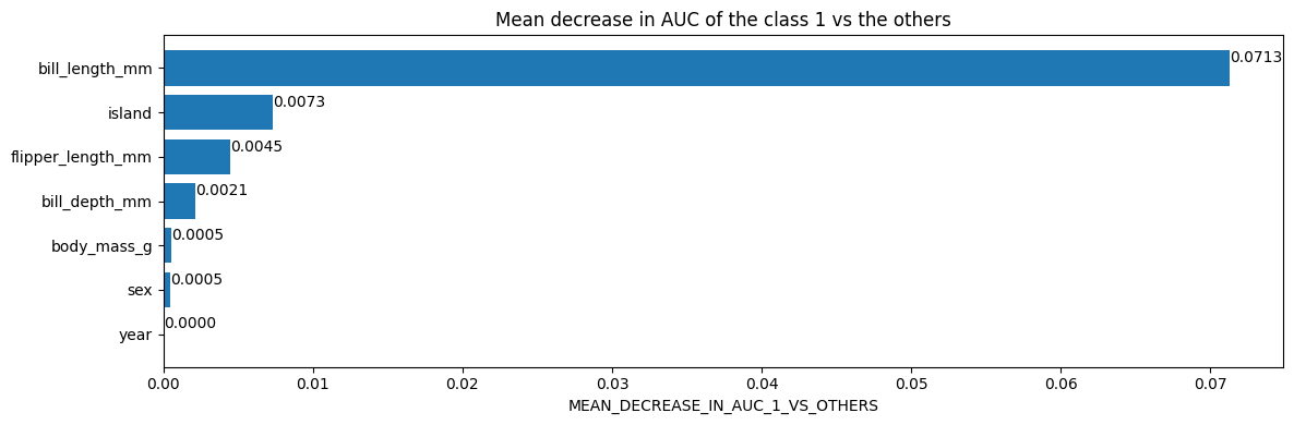
Different variable importances have different semantics. For example, a feature
with a mean decrease in auc of 0.05 means that removing this feature from
the training dataset would reduce/hurt the AUC by 5%.
# Mean decrease in AUC of the class 1 vs the others.
inspector.variable_importances()["MEAN_DECREASE_IN_AUC_1_VS_OTHERS"]
[("bill_length_mm" (1; #2), 0.0713061951754389),
 ("island" (4; #5), 0.007298519736842035),
 ("flipper_length_mm" (1; #4), 0.004505893640351366),
 ("bill_depth_mm" (1; #1), 0.0021244517543865804),
 ("body_mass_g" (1; #3), 0.0005482456140351033),
 ("sex" (4; #6), 0.00047971491228060437),
 ("year" (1; #7), 0.0)]
Plot the variable importances from the inspector using Matplotlib
import matplotlib.pyplot as plt

plt.figure(figsize=(12, 4))

# Mean decrease in AUC of the class 1 vs the others.
variable_importance_metric = "MEAN_DECREASE_IN_AUC_1_VS_OTHERS"
variable_importances = inspector.variable_importances()[variable_importance_metric]

# Extract the feature name and importance values.
#
# `variable_importances` is a list of <feature, importance> tuples.
feature_names = [vi[0].name for vi in variable_importances]
feature_importances = [vi[1] for vi in variable_importances]
# The feature are ordered in decreasing importance value.
feature_ranks = range(len(feature_names))

bar = plt.barh(feature_ranks, feature_importances, label=[str(x) for x in feature_ranks])
plt.yticks(feature_ranks, feature_names)
plt.gca().invert_yaxis()

# TODO: Replace with "plt.bar_label()" when available.
# Label each bar with values
for importance, patch in zip(feature_importances, bar.patches):
  plt.text(patch.get_x() + patch.get_width(), patch.get_y(), f"{importance:.4f}", va="top")

plt.xlabel(variable_importance_metric)
plt.title("Mean decrease in AUC of the class 1 vs the others")
plt.tight_layout()
plt.show()
Finally, access the actual tree structure:
inspector.extract_tree(tree_idx=0)
Tree(root=NonLeafNode(condition=(bill_length_mm >= 43.25; miss=True, score=0.5482327342033386), pos_child=NonLeafNode(condition=(island in ['Biscoe']; miss=True, score=0.6515106558799744), pos_child=NonLeafNode(condition=(bill_depth_mm >= 17.225584030151367; miss=False, score=0.027205035090446472), pos_child=LeafNode(value=ProbabilityValue([0.16666666666666666, 0.0, 0.8333333333333334],n=6.0), idx=7), neg_child=LeafNode(value=ProbabilityValue([0.0, 0.0, 1.0],n=104.0), idx=6), value=ProbabilityValue([0.00909090909090909, 0.0, 0.990909090909091],n=110.0)), neg_child=LeafNode(value=ProbabilityValue([0.0, 1.0, 0.0],n=61.0), idx=5), value=ProbabilityValue([0.005847953216374269, 0.3567251461988304, 0.6374269005847953],n=171.0)), neg_child=NonLeafNode(condition=(bill_depth_mm >= 15.100000381469727; miss=True, score=0.150658518075943), pos_child=NonLeafNode(condition=(flipper_length_mm >= 187.5; miss=True, score=0.036139510571956635), pos_child=LeafNode(value=ProbabilityValue([1.0, 0.0, 0.0],n=104.0), idx=4), neg_child=NonLeafNode(condition=(bill_length_mm >= 42.30000305175781; miss=True, score=0.23430533707141876), pos_child=LeafNode(value=ProbabilityValue([0.0, 1.0, 0.0],n=5.0), idx=3), neg_child=NonLeafNode(condition=(bill_length_mm >= 40.55000305175781; miss=True, score=0.043961383402347565), pos_child=LeafNode(value=ProbabilityValue([0.8, 0.2, 0.0],n=5.0), idx=2), neg_child=LeafNode(value=ProbabilityValue([1.0, 0.0, 0.0],n=53.0), idx=1), value=ProbabilityValue([0.9827586206896551, 0.017241379310344827, 0.0],n=58.0)), value=ProbabilityValue([0.9047619047619048, 0.09523809523809523, 0.0],n=63.0)), value=ProbabilityValue([0.9640718562874252, 0.03592814371257485, 0.0],n=167.0)), neg_child=LeafNode(value=ProbabilityValue([0.0, 0.0, 1.0],n=6.0), idx=0), value=ProbabilityValue([0.930635838150289, 0.03468208092485549, 0.03468208092485549],n=173.0)), value=ProbabilityValue([0.47093023255813954, 0.19476744186046513, 0.33430232558139533],n=344.0)), label_classes=None)
Extracting a tree is not efficient. If speed is important, the model inspection can be done with the iterate_on_nodes() method instead. This method is a Depth First Pre-order traversals iterator on all the nodes of the model.
For following example computes how many times each feature is used (this is a kind of structural variable importance):
# number_of_use[F] will be the number of node using feature F in its condition.
number_of_use = collections.defaultdict(lambda: 0)

# Iterate over all the nodes in a Depth First Pre-order traversals.
for node_iter in inspector.iterate_on_nodes():

  if not isinstance(node_iter.node, tfdf.py_tree.node.NonLeafNode):
    # Skip the leaf nodes
    continue

  # Iterate over all the features used in the condition.
  # By default, models are "oblique" i.e. each node tests a single feature.
  for feature in node_iter.node.condition.features():
    number_of_use[feature] += 1

print("Number of condition nodes per features:")
for feature, count in number_of_use.items():
  print("\t", feature.name, ":", count)
Number of condition nodes per features:
     bill_length_mm : 778
     bill_depth_mm : 463
     flipper_length_mm : 414
     island : 342
     body_mass_g : 338
     year : 19
     sex : 36
Creating a model by hand
In this section you will create a small Random Forest model by hand. To make it extra easy, the model will only contain one simple tree:
3 label classes: Red, blue and green.
2 features: f1 (numerical) and f2 (string categorical)

f1>=1.5
    ├─(pos)─ f2 in ["cat","dog"]
    │         ├─(pos)─ value: [0.8, 0.1, 0.1]
    │         └─(neg)─ value: [0.1, 0.8, 0.1]
    └─(neg)─ value: [0.1, 0.1, 0.8]
# Create the model builder
builder = tfdf.builder.RandomForestBuilder(
    path="/tmp/manual_model",
    objective=tfdf.py_tree.objective.ClassificationObjective(
        label="color", classes=["red", "blue", "green"]))
Each tree is added one by one.
# So alias
Tree = tfdf.py_tree.tree.Tree
SimpleColumnSpec = tfdf.py_tree.dataspec.SimpleColumnSpec
ColumnType = tfdf.py_tree.dataspec.ColumnType
# Nodes
NonLeafNode = tfdf.py_tree.node.NonLeafNode
LeafNode = tfdf.py_tree.node.LeafNode
# Conditions
NumericalHigherThanCondition = tfdf.py_tree.condition.NumericalHigherThanCondition
CategoricalIsInCondition = tfdf.py_tree.condition.CategoricalIsInCondition
# Leaf values
ProbabilityValue = tfdf.py_tree.value.ProbabilityValue

builder.add_tree(
    Tree(
        NonLeafNode(
            condition=NumericalHigherThanCondition(
                feature=SimpleColumnSpec(name="f1", type=ColumnType.NUMERICAL),
                threshold=1.5,
                missing_evaluation=False),
            pos_child=NonLeafNode(
                condition=CategoricalIsInCondition(
                    feature=SimpleColumnSpec(name="f2",type=ColumnType.CATEGORICAL),
                    mask=["cat", "dog"],
                    missing_evaluation=False),
                pos_child=LeafNode(value=ProbabilityValue(probability=[0.8, 0.1, 0.1], num_examples=10)),
                neg_child=LeafNode(value=ProbabilityValue(probability=[0.1, 0.8, 0.1], num_examples=20))),
            neg_child=LeafNode(value=ProbabilityValue(probability=[0.1, 0.1, 0.8], num_examples=30)))))
Conclude the tree writing
builder.close()
[INFO 24-03-15 11:31:03.0647 UTC kernel.cc:1233] Loading model from path /tmp/manual_model/tmp/ with prefix d19dedc1225c428c
[INFO 24-03-15 11:31:03.0650 UTC decision_forest.cc:734] Model loaded with 1 root(s), 5 node(s), and 2 input feature(s).
[INFO 24-03-15 11:31:03.0650 UTC kernel.cc:1061] Use fast generic engine
INFO:tensorflow:Assets written to: /tmp/manual_model/assets
INFO:tensorflow:Assets written to: /tmp/manual_model/assets
Now you can open the model as a regular keras model, and make predictions:
manual_model = tf_keras.models.load_model("/tmp/manual_model")
[INFO 24-03-15 11:31:04.2493 UTC kernel.cc:1233] Loading model from path /tmp/manual_model/assets/ with prefix d19dedc1225c428c
[INFO 24-03-15 11:31:04.2496 UTC decision_forest.cc:734] Model loaded with 1 root(s), 5 node(s), and 2 input feature(s).
[INFO 24-03-15 11:31:04.2497 UTC kernel.cc:1061] Use fast generic engine
examples = tf.data.Dataset.from_tensor_slices({
        "f1": [1.0, 2.0, 3.0],
        "f2": ["cat", "cat", "bird"]
    }).batch(2)

predictions = manual_model.predict(examples)

print("predictions:\n",predictions)
2/2 [==============================] - 1s 3ms/step
predictions:
 [[0.1 0.1 0.8]
 [0.8 0.1 0.1]
 [0.1 0.8 0.1]]
Access the structure:
yggdrasil_model_path = manual_model.yggdrasil_model_path_tensor().numpy().decode("utf-8")
print("yggdrasil_model_path:",yggdrasil_model_path)

inspector = tfdf.inspector.make_inspector(yggdrasil_model_path)
print("Input features:", inspector.features())
yggdrasil_model_path: /tmp/manual_model/assets/
Input features: ["f1" (1; #1), "f2" (4; #2)]
And of course, you can plot this manually constructed model:
tfdf.model_plotter.plot_model_in_colab(manual_model)