
|
|
|
 View source on GitHub
|
|
This tutorial demonstrates training a simple Convolutional Neural Network (CNN) to classify CIFAR images. Because this tutorial uses the Keras Sequential API, creating and training your model will take just a few lines of code.
Import TensorFlow
import tensorflow as tf

from tensorflow.keras import datasets, layers, models
import matplotlib.pyplot as plt
2023-10-27 06:01:15.153603: E external/local_xla/xla/stream_executor/cuda/cuda_dnn.cc:9261] Unable to register cuDNN factory: Attempting to register factory for plugin cuDNN when one has already been registered
2023-10-27 06:01:15.153656: E external/local_xla/xla/stream_executor/cuda/cuda_fft.cc:607] Unable to register cuFFT factory: Attempting to register factory for plugin cuFFT when one has already been registered
2023-10-27 06:01:15.155401: E external/local_xla/xla/stream_executor/cuda/cuda_blas.cc:1515] Unable to register cuBLAS factory: Attempting to register factory for plugin cuBLAS when one has already been registered
Download and prepare the CIFAR10 dataset
The CIFAR10 dataset contains 60,000 color images in 10 classes, with 6,000 images in each class. The dataset is divided into 50,000 training images and 10,000 testing images. The classes are mutually exclusive and there is no overlap between them.
(train_images, train_labels), (test_images, test_labels) = datasets.cifar10.load_data()

# Normalize pixel values to be between 0 and 1
train_images, test_images = train_images / 255.0, test_images / 255.0
Downloading data from https://www.cs.toronto.edu/~kriz/cifar-10-python.tar.gz
170498071/170498071 [==============================] - 2s 0us/step
Verify the data
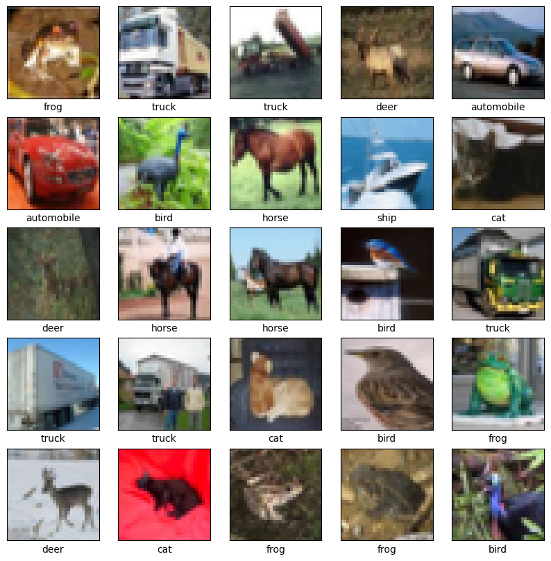
To verify that the dataset looks correct, let's plot the first 25 images from the training set and display the class name below each image:
class_names = ['airplane', 'automobile', 'bird', 'cat', 'deer',
               'dog', 'frog', 'horse', 'ship', 'truck']

plt.figure(figsize=(10,10))
for i in range(25):
    plt.subplot(5,5,i+1)
    plt.xticks([])
    plt.yticks([])
    plt.grid(False)
    plt.imshow(train_images[i])
    # The CIFAR labels happen to be arrays,
    # which is why you need the extra index
    plt.xlabel(class_names[train_labels[i][0]])
plt.show()
Create the convolutional base
The 6 lines of code below define the convolutional base using a common pattern: a stack of Conv2D and MaxPooling2D layers.
As input, a CNN takes tensors of shape (image_height, image_width, color_channels), ignoring the batch size. If you are new to these dimensions, color_channels refers to (R,G,B). In this example, you will configure your CNN to process inputs of shape (32, 32, 3), which is the format of CIFAR images. You can do this by passing the argument input_shape to your first layer.
model = models.Sequential()
model.add(layers.Conv2D(32, (3, 3), activation='relu', input_shape=(32, 32, 3)))
model.add(layers.MaxPooling2D((2, 2)))
model.add(layers.Conv2D(64, (3, 3), activation='relu'))
model.add(layers.MaxPooling2D((2, 2)))
model.add(layers.Conv2D(64, (3, 3), activation='relu'))
Let's display the architecture of your model so far:
model.summary()
Model: "sequential"
_________________________________________________________________
 Layer (type)                Output Shape              Param #
=================================================================
 conv2d (Conv2D)             (None, 30, 30, 32)        896

 max_pooling2d (MaxPooling2  (None, 15, 15, 32)        0
 D)

 conv2d_1 (Conv2D)           (None, 13, 13, 64)        18496

 max_pooling2d_1 (MaxPoolin  (None, 6, 6, 64)          0
 g2D)

 conv2d_2 (Conv2D)           (None, 4, 4, 64)          36928

=================================================================
Total params: 56320 (220.00 KB)
Trainable params: 56320 (220.00 KB)
Non-trainable params: 0 (0.00 Byte)
_________________________________________________________________
Above, you can see that the output of every Conv2D and MaxPooling2D layer is a 3D tensor of shape (height, width, channels). The width and height dimensions tend to shrink as you go deeper in the network. The number of output channels for each Conv2D layer is controlled by the first argument (e.g., 32 or 64). Typically, as the width and height shrink, you can afford (computationally) to add more output channels in each Conv2D layer.
Add Dense layers on top
To complete the model, you will feed the last output tensor from the convolutional base (of shape (4, 4, 64)) into one or more Dense layers to perform classification. Dense layers take vectors as input (which are 1D), while the current output is a 3D tensor. First, you will flatten (or unroll) the 3D output to 1D, then add one or more Dense layers on top. CIFAR has 10 output classes, so you use a final Dense layer with 10 outputs.
model.add(layers.Flatten())
model.add(layers.Dense(64, activation='relu'))
model.add(layers.Dense(10))
Here's the complete architecture of your model:
model.summary()
Model: "sequential"
_________________________________________________________________
 Layer (type)                Output Shape              Param #
=================================================================
 conv2d (Conv2D)             (None, 30, 30, 32)        896

 max_pooling2d (MaxPooling2  (None, 15, 15, 32)        0
 D)

 conv2d_1 (Conv2D)           (None, 13, 13, 64)        18496

 max_pooling2d_1 (MaxPoolin  (None, 6, 6, 64)          0
 g2D)

 conv2d_2 (Conv2D)           (None, 4, 4, 64)          36928

 flatten (Flatten)           (None, 1024)              0

 dense (Dense)               (None, 64)                65600

 dense_1 (Dense)             (None, 10)                650

=================================================================
Total params: 122570 (478.79 KB)
Trainable params: 122570 (478.79 KB)
Non-trainable params: 0 (0.00 Byte)
_________________________________________________________________
The network summary shows that (4, 4, 64) outputs were flattened into vectors of shape (1024) before going through two Dense layers.
Compile and train the model
model.compile(optimizer='adam',
              loss=tf.keras.losses.SparseCategoricalCrossentropy(from_logits=True),
              metrics=['accuracy'])

history = model.fit(train_images, train_labels, epochs=10,
                    validation_data=(test_images, test_labels))
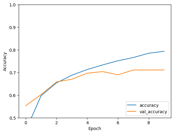
Epoch 1/10
WARNING: All log messages before absl::InitializeLog() is called are written to STDERR
I0000 00:00:1698386490.372362  489369 device_compiler.h:186] Compiled cluster using XLA!  This line is logged at most once for the lifetime of the process.
1563/1563 [==============================] - 10s 5ms/step - loss: 1.5211 - accuracy: 0.4429 - val_loss: 1.2497 - val_accuracy: 0.5531
Epoch 2/10
1563/1563 [==============================] - 6s 4ms/step - loss: 1.1408 - accuracy: 0.5974 - val_loss: 1.1474 - val_accuracy: 0.6023
Epoch 3/10
1563/1563 [==============================] - 6s 4ms/step - loss: 0.9862 - accuracy: 0.6538 - val_loss: 0.9759 - val_accuracy: 0.6582
Epoch 4/10
1563/1563 [==============================] - 6s 4ms/step - loss: 0.8929 - accuracy: 0.6879 - val_loss: 0.9412 - val_accuracy: 0.6702
Epoch 5/10
1563/1563 [==============================] - 6s 4ms/step - loss: 0.8183 - accuracy: 0.7131 - val_loss: 0.8830 - val_accuracy: 0.6967
Epoch 6/10
1563/1563 [==============================] - 6s 4ms/step - loss: 0.7588 - accuracy: 0.7334 - val_loss: 0.8671 - val_accuracy: 0.7039
Epoch 7/10
1563/1563 [==============================] - 6s 4ms/step - loss: 0.7126 - accuracy: 0.7518 - val_loss: 0.8972 - val_accuracy: 0.6897
Epoch 8/10
1563/1563 [==============================] - 7s 4ms/step - loss: 0.6655 - accuracy: 0.7661 - val_loss: 0.8412 - val_accuracy: 0.7111
Epoch 9/10
1563/1563 [==============================] - 7s 4ms/step - loss: 0.6205 - accuracy: 0.7851 - val_loss: 0.8581 - val_accuracy: 0.7109
Epoch 10/10
1563/1563 [==============================] - 7s 4ms/step - loss: 0.5872 - accuracy: 0.7937 - val_loss: 0.8817 - val_accuracy: 0.7113
Evaluate the model
plt.plot(history.history['accuracy'], label='accuracy')
plt.plot(history.history['val_accuracy'], label = 'val_accuracy')
plt.xlabel('Epoch')
plt.ylabel('Accuracy')
plt.ylim([0.5, 1])
plt.legend(loc='lower right')

test_loss, test_acc = model.evaluate(test_images,  test_labels, verbose=2)
313/313 - 1s - loss: 0.8817 - accuracy: 0.7113 - 655ms/epoch - 2ms/step
print(test_acc)
0.7113000154495239
Your simple CNN has achieved a test accuracy of over 70%. Not bad for a few lines of code! For another CNN style, check out the TensorFlow 2 quickstart for experts example that uses the Keras subclassing API and tf.GradientTape.