
| | |  הצג ב-GitHub הצג ב-GitHub | |
ביישומי AI שהם קריטיים לבטיחות (למשל, קבלת החלטות רפואיות ונהיגה אוטונומית) או שבהם הנתונים רועשים מטבעם (למשל, הבנת שפה טבעית), חשוב למסווג עמוק לכמת באופן אמין את אי הוודאות שלו. המסווג העמוק צריך להיות מודע למגבלותיו שלו ומתי עליו להעביר את השליטה לידי המומחים האנושיים. מדריך זה מראה כיצד לשפר את יכולתו של מסווג עמוק בכימות אי ודאות באמצעות טכניקה הנקראת Spectral-normalized Neural Gaussian Process ( SNGP ) .
הרעיון המרכזי של SNGP הוא לשפר את מודעות המרחק של מסווג עמוק על ידי החלת שינויים פשוטים ברשת. מודעות למרחק של מודל היא מדד לאופן שבו ההסתברות החזויה שלו משקפת את המרחק בין דוגמא המבחן לנתוני האימון. זהו תכונה רצויה המקובלת למודלים הסתברותיים בסטנדרט זהב (למשל, תהליך גאוס עם גרעיני RBF) אך חסרה במודלים עם רשתות עצביות עמוקות. SNGP מספק דרך פשוטה להחדיר את התנהגות תהליך גאוס למסווג עמוק תוך שמירה על דיוק הניבוי שלו.
מדריך זה מיישם מודל SNGP מבוסס רשת שיורית עמוקה (ResNet) על מערך הנתונים של שני ירחים , ומשווה את משטח אי הוודאות שלו לזה של שתי גישות אי-ודאות פופולריות אחרות - נשירה של מונטה קרלו ו- Deep ensemble .
מדריך זה ממחיש את מודל SNGP על מערך צעצוע דו-ממדי. לדוגמא של יישום SNGP על משימת הבנת שפה טבעית בעולם האמיתי באמצעות BERT-base, עיין במדריך SNGP-BERT . להטמעות באיכות גבוהה של מודל SNGP (ושיטות רבות אחרות של אי ודאות) במגוון רחב של מערכי נתונים בנצ'מרק (למשל, CIFAR-100 , ImageNet , זיהוי רעילות של Jigsaw וכו'), אנא עיין במדד אי- הוודאות Baselines .
על SNGP
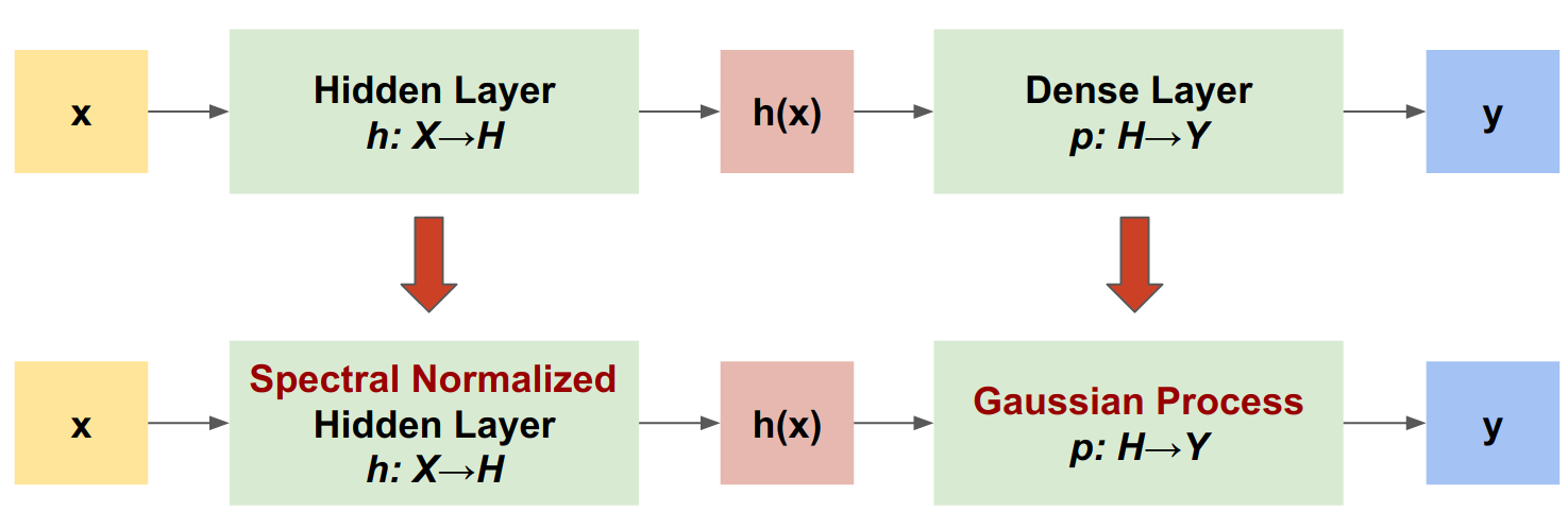
תהליך גאוס עצבי מנורמל ספקטרלי (SNGP) היא גישה פשוטה לשיפור איכות אי הוודאות של מסווג עמוק תוך שמירה על רמה דומה של דיוק והשהייה. בהינתן רשת שיורית עמוקה, SNGP מבצעת שני שינויים פשוטים במודל:
- הוא מחיל נורמליזציה ספקטרלית על השכבות השיוריות הנסתרות.
- הוא מחליף את שכבת הפלט הצפופה בשכבת תהליך גאוסי.
בהשוואה לגישות אי-ודאות אחרות (למשל, נשירה של מונטה קרלו או אנסמבל Deep), ל-SNGP מספר יתרונות:
- זה עובד עבור מגוון רחב של ארכיטקטורות המבוססות שאריות חדישות (למשל, (Wide) ResNet, DenseNet, BERT וכו').
- זוהי שיטה של מודל יחיד (כלומר, אינה מסתמכת על ממוצע אנסמבל). לכן ל-SNGP יש רמת חביון דומה לרשת דטרמיניסטית יחידה, וניתן להתאים אותה בקלות למערכי נתונים גדולים כמו ImageNet ו- Jigsaw Toxic Comments סיווג .
- יש לו ביצועי זיהוי חזקים מחוץ לתחום הודות לתכונת המודעות למרחק .
החסרונות של שיטה זו הם:
אי הוודאות הניבוי של SNGP מחושבת באמצעות קירוב Laplace . לכן תיאורטית, אי הוודאות האחורית של SNGP שונה מזו של תהליך גאוסי מדויק.
אימון SNGP זקוק לשלב איפוס שיתוף פעולה בתחילת עידן חדש. זה יכול להוסיף כמות זעירה של מורכבות נוספת לצינור האימונים. מדריך זה מראה דרך פשוטה ליישם זאת באמצעות התקשרויות חוזרות של Keras.
להכין
pip install --use-deprecated=legacy-resolver tf-models-official
# refresh pkg_resources so it takes the changes into account.
import pkg_resources
import importlib
importlib.reload(pkg_resources)
<module 'pkg_resources' from '/tmpfs/src/tf_docs_env/lib/python3.7/site-packages/pkg_resources/__init__.py'>
import matplotlib.pyplot as plt
import matplotlib.colors as colors

import sklearn.datasets

import numpy as np
import tensorflow as tf

import official.nlp.modeling.layers as nlp_layers
הגדר פקודות מאקרו להדמיה
plt.rcParams['figure.dpi'] = 140

DEFAULT_X_RANGE = (-3.5, 3.5)
DEFAULT_Y_RANGE = (-2.5, 2.5)
DEFAULT_CMAP = colors.ListedColormap(["#377eb8", "#ff7f00"])
DEFAULT_NORM = colors.Normalize(vmin=0, vmax=1,)
DEFAULT_N_GRID = 100
מערך הנתונים של שני הירחים
צור את מערכי ההדרכה וההערכה ממערך הנתונים של שני הירחים .
def make_training_data(sample_size=500):
  """Create two moon training dataset."""
  train_examples, train_labels = sklearn.datasets.make_moons(
      n_samples=2 * sample_size, noise=0.1)

  # Adjust data position slightly.
  train_examples[train_labels == 0] += [-0.1, 0.2]
  train_examples[train_labels == 1] += [0.1, -0.2]

  return train_examples, train_labels
הערך את ההתנהגות החזויה של המודל על פני כל מרחב הקלט הדו-ממדי.
def make_testing_data(x_range=DEFAULT_X_RANGE, y_range=DEFAULT_Y_RANGE, n_grid=DEFAULT_N_GRID):
  """Create a mesh grid in 2D space."""
  # testing data (mesh grid over data space)
  x = np.linspace(x_range[0], x_range[1], n_grid)
  y = np.linspace(y_range[0], y_range[1], n_grid)
  xv, yv = np.meshgrid(x, y)
  return np.stack([xv.flatten(), yv.flatten()], axis=-1)
כדי להעריך אי ודאות במודל, הוסף מערך נתונים מחוץ לתחום (OOD) השייך למחלקה שלישית. המודל אף פעם לא רואה את דוגמאות ה-OOD הללו במהלך האימון.
def make_ood_data(sample_size=500, means=(2.5, -1.75), vars=(0.01, 0.01)):
  return np.random.multivariate_normal(
      means, cov=np.diag(vars), size=sample_size)
# Load the train, test and OOD datasets.
train_examples, train_labels = make_training_data(
    sample_size=500)
test_examples = make_testing_data()
ood_examples = make_ood_data(sample_size=500)

# Visualize
pos_examples = train_examples[train_labels == 0]
neg_examples = train_examples[train_labels == 1]

plt.figure(figsize=(7, 5.5))

plt.scatter(pos_examples[:, 0], pos_examples[:, 1], c="#377eb8", alpha=0.5)
plt.scatter(neg_examples[:, 0], neg_examples[:, 1], c="#ff7f00", alpha=0.5)
plt.scatter(ood_examples[:, 0], ood_examples[:, 1], c="red", alpha=0.1)

plt.legend(["Postive", "Negative", "Out-of-Domain"])

plt.ylim(DEFAULT_Y_RANGE)
plt.xlim(DEFAULT_X_RANGE)

plt.show()

כאן הכחול והכתום מייצגים את המחלקות החיוביות והשליליות, והאדום מייצג את נתוני ה-OOD. מודל שמכמת היטב את אי הוודאות צפוי להיות בטוח כשהוא קרוב לנתוני אימון (כלומר, \(p(x_{test})\) קרוב ל-0 או 1), ולהיות לא בטוח כשהוא רחוק מאזורי נתוני האימון (כלומר, \(p(x_{test})\) קרוב ל-0.5 ).
המודל הדטרמיניסטי
הגדר מודל
התחל מהמודל הדטרמיניסטי (הבסיסי): רשת שיורית רב-שכבתית (ResNet) עם הסדרת נשירה.
class DeepResNet(tf.keras.Model):
  """Defines a multi-layer residual network."""
  def __init__(self, num_classes, num_layers=3, num_hidden=128,
               dropout_rate=0.1, **classifier_kwargs):
    super().__init__()
    # Defines class meta data.
    self.num_hidden = num_hidden
    self.num_layers = num_layers
    self.dropout_rate = dropout_rate
    self.classifier_kwargs = classifier_kwargs

    # Defines the hidden layers.
    self.input_layer = tf.keras.layers.Dense(self.num_hidden, trainable=False)
    self.dense_layers = [self.make_dense_layer() for _ in range(num_layers)]

    # Defines the output layer.
    self.classifier = self.make_output_layer(num_classes)

  def call(self, inputs):
    # Projects the 2d input data to high dimension.
    hidden = self.input_layer(inputs)

    # Computes the resnet hidden representations.
    for i in range(self.num_layers):
      resid = self.dense_layers[i](hidden)
      resid = tf.keras.layers.Dropout(self.dropout_rate)(resid)
      hidden += resid

    return self.classifier(hidden)

  def make_dense_layer(self):
    """Uses the Dense layer as the hidden layer."""
    return tf.keras.layers.Dense(self.num_hidden, activation="relu")

  def make_output_layer(self, num_classes):
    """Uses the Dense layer as the output layer."""
    return tf.keras.layers.Dense(
        num_classes, **self.classifier_kwargs)
מדריך זה משתמש ב-ResNet בן 6 שכבות עם 128 יחידות נסתרות.
resnet_config = dict(num_classes=2, num_layers=6, num_hidden=128)
resnet_model = DeepResNet(**resnet_config)
resnet_model.build((None, 2))
resnet_model.summary()
Model: "deep_res_net"
_________________________________________________________________
 Layer (type)                Output Shape              Param #
=================================================================
 dense (Dense)               multiple                  384

 dense_1 (Dense)             multiple                  16512

 dense_2 (Dense)             multiple                  16512

 dense_3 (Dense)             multiple                  16512

 dense_4 (Dense)             multiple                  16512

 dense_5 (Dense)             multiple                  16512

 dense_6 (Dense)             multiple                  16512

 dense_7 (Dense)             multiple                  258

=================================================================
Total params: 99,714
Trainable params: 99,330
Non-trainable params: 384
_________________________________________________________________
דגם רכבת
הגדר את פרמטרי האימון כך שישתמשו ב- SparseCategoricalCrossentropy ההפסד ובאופטימיזציית Adam.
loss = tf.keras.losses.SparseCategoricalCrossentropy(from_logits=True)
metrics = tf.keras.metrics.SparseCategoricalAccuracy(),
optimizer = tf.keras.optimizers.Adam(learning_rate=1e-4)

train_config = dict(loss=loss, metrics=metrics, optimizer=optimizer)
אמן את הדגם למשך 100 עידנים עם גודל אצווה 128.
fit_config = dict(batch_size=128, epochs=100)
resnet_model.compile(**train_config)
resnet_model.fit(train_examples, train_labels, **fit_config)
Epoch 1/100
8/8 [==============================] - 1s 4ms/step - loss: 1.1251 - sparse_categorical_accuracy: 0.5050
Epoch 2/100
8/8 [==============================] - 0s 3ms/step - loss: 0.5538 - sparse_categorical_accuracy: 0.6920
Epoch 3/100
8/8 [==============================] - 0s 3ms/step - loss: 0.2881 - sparse_categorical_accuracy: 0.9160
Epoch 4/100
8/8 [==============================] - 0s 3ms/step - loss: 0.1923 - sparse_categorical_accuracy: 0.9370
Epoch 5/100
8/8 [==============================] - 0s 3ms/step - loss: 0.1550 - sparse_categorical_accuracy: 0.9420
Epoch 6/100
8/8 [==============================] - 0s 3ms/step - loss: 0.1403 - sparse_categorical_accuracy: 0.9450
Epoch 7/100
8/8 [==============================] - 0s 3ms/step - loss: 0.1269 - sparse_categorical_accuracy: 0.9430
Epoch 8/100
8/8 [==============================] - 0s 3ms/step - loss: 0.1208 - sparse_categorical_accuracy: 0.9460
Epoch 9/100
8/8 [==============================] - 0s 3ms/step - loss: 0.1158 - sparse_categorical_accuracy: 0.9510
Epoch 10/100
8/8 [==============================] - 0s 3ms/step - loss: 0.1103 - sparse_categorical_accuracy: 0.9490
Epoch 11/100
8/8 [==============================] - 0s 3ms/step - loss: 0.1051 - sparse_categorical_accuracy: 0.9510
Epoch 12/100
8/8 [==============================] - 0s 3ms/step - loss: 0.1053 - sparse_categorical_accuracy: 0.9510
Epoch 13/100
8/8 [==============================] - 0s 3ms/step - loss: 0.1013 - sparse_categorical_accuracy: 0.9450
Epoch 14/100
8/8 [==============================] - 0s 4ms/step - loss: 0.0967 - sparse_categorical_accuracy: 0.9500
Epoch 15/100
8/8 [==============================] - 0s 3ms/step - loss: 0.0991 - sparse_categorical_accuracy: 0.9530
Epoch 16/100
8/8 [==============================] - 0s 3ms/step - loss: 0.0984 - sparse_categorical_accuracy: 0.9500
Epoch 17/100
8/8 [==============================] - 0s 3ms/step - loss: 0.0982 - sparse_categorical_accuracy: 0.9480
Epoch 18/100
8/8 [==============================] - 0s 4ms/step - loss: 0.0918 - sparse_categorical_accuracy: 0.9510
Epoch 19/100
8/8 [==============================] - 0s 3ms/step - loss: 0.0903 - sparse_categorical_accuracy: 0.9500
Epoch 20/100
8/8 [==============================] - 0s 3ms/step - loss: 0.0883 - sparse_categorical_accuracy: 0.9510
Epoch 21/100
8/8 [==============================] - 0s 3ms/step - loss: 0.0870 - sparse_categorical_accuracy: 0.9530
Epoch 22/100
8/8 [==============================] - 0s 3ms/step - loss: 0.0884 - sparse_categorical_accuracy: 0.9560
Epoch 23/100
8/8 [==============================] - 0s 3ms/step - loss: 0.0850 - sparse_categorical_accuracy: 0.9540
Epoch 24/100
8/8 [==============================] - 0s 3ms/step - loss: 0.0808 - sparse_categorical_accuracy: 0.9580
Epoch 25/100
8/8 [==============================] - 0s 3ms/step - loss: 0.0773 - sparse_categorical_accuracy: 0.9560
Epoch 26/100
8/8 [==============================] - 0s 3ms/step - loss: 0.0801 - sparse_categorical_accuracy: 0.9590
Epoch 27/100
8/8 [==============================] - 0s 3ms/step - loss: 0.0779 - sparse_categorical_accuracy: 0.9580
Epoch 28/100
8/8 [==============================] - 0s 3ms/step - loss: 0.0807 - sparse_categorical_accuracy: 0.9580
Epoch 29/100
8/8 [==============================] - 0s 3ms/step - loss: 0.0820 - sparse_categorical_accuracy: 0.9570
Epoch 30/100
8/8 [==============================] - 0s 3ms/step - loss: 0.0730 - sparse_categorical_accuracy: 0.9600
Epoch 31/100
8/8 [==============================] - 0s 3ms/step - loss: 0.0782 - sparse_categorical_accuracy: 0.9590
Epoch 32/100
8/8 [==============================] - 0s 4ms/step - loss: 0.0704 - sparse_categorical_accuracy: 0.9600
Epoch 33/100
8/8 [==============================] - 0s 3ms/step - loss: 0.0709 - sparse_categorical_accuracy: 0.9610
Epoch 34/100
8/8 [==============================] - 0s 3ms/step - loss: 0.0758 - sparse_categorical_accuracy: 0.9580
Epoch 35/100
8/8 [==============================] - 0s 3ms/step - loss: 0.0702 - sparse_categorical_accuracy: 0.9610
Epoch 36/100
8/8 [==============================] - 0s 3ms/step - loss: 0.0688 - sparse_categorical_accuracy: 0.9600
Epoch 37/100
8/8 [==============================] - 0s 3ms/step - loss: 0.0675 - sparse_categorical_accuracy: 0.9630
Epoch 38/100
8/8 [==============================] - 0s 3ms/step - loss: 0.0636 - sparse_categorical_accuracy: 0.9690
Epoch 39/100
8/8 [==============================] - 0s 3ms/step - loss: 0.0677 - sparse_categorical_accuracy: 0.9610
Epoch 40/100
8/8 [==============================] - 0s 3ms/step - loss: 0.0702 - sparse_categorical_accuracy: 0.9650
Epoch 41/100
8/8 [==============================] - 0s 3ms/step - loss: 0.0614 - sparse_categorical_accuracy: 0.9690
Epoch 42/100
8/8 [==============================] - 0s 3ms/step - loss: 0.0663 - sparse_categorical_accuracy: 0.9680
Epoch 43/100
8/8 [==============================] - 0s 3ms/step - loss: 0.0626 - sparse_categorical_accuracy: 0.9740
Epoch 44/100
8/8 [==============================] - 0s 3ms/step - loss: 0.0590 - sparse_categorical_accuracy: 0.9760
Epoch 45/100
8/8 [==============================] - 0s 3ms/step - loss: 0.0573 - sparse_categorical_accuracy: 0.9780
Epoch 46/100
8/8 [==============================] - 0s 3ms/step - loss: 0.0568 - sparse_categorical_accuracy: 0.9770
Epoch 47/100
8/8 [==============================] - 0s 3ms/step - loss: 0.0595 - sparse_categorical_accuracy: 0.9780
Epoch 48/100
8/8 [==============================] - 0s 3ms/step - loss: 0.0482 - sparse_categorical_accuracy: 0.9840
Epoch 49/100
8/8 [==============================] - 0s 3ms/step - loss: 0.0515 - sparse_categorical_accuracy: 0.9820
Epoch 50/100
8/8 [==============================] - 0s 3ms/step - loss: 0.0525 - sparse_categorical_accuracy: 0.9830
Epoch 51/100
8/8 [==============================] - 0s 3ms/step - loss: 0.0507 - sparse_categorical_accuracy: 0.9790
Epoch 52/100
8/8 [==============================] - 0s 3ms/step - loss: 0.0433 - sparse_categorical_accuracy: 0.9850
Epoch 53/100
8/8 [==============================] - 0s 3ms/step - loss: 0.0511 - sparse_categorical_accuracy: 0.9820
Epoch 54/100
8/8 [==============================] - 0s 3ms/step - loss: 0.0501 - sparse_categorical_accuracy: 0.9820
Epoch 55/100
8/8 [==============================] - 0s 3ms/step - loss: 0.0440 - sparse_categorical_accuracy: 0.9890
Epoch 56/100
8/8 [==============================] - 0s 3ms/step - loss: 0.0438 - sparse_categorical_accuracy: 0.9850
Epoch 57/100
8/8 [==============================] - 0s 3ms/step - loss: 0.0438 - sparse_categorical_accuracy: 0.9880
Epoch 58/100
8/8 [==============================] - 0s 3ms/step - loss: 0.0416 - sparse_categorical_accuracy: 0.9860
Epoch 59/100
8/8 [==============================] - 0s 3ms/step - loss: 0.0479 - sparse_categorical_accuracy: 0.9860
Epoch 60/100
8/8 [==============================] - 0s 3ms/step - loss: 0.0434 - sparse_categorical_accuracy: 0.9860
Epoch 61/100
8/8 [==============================] - 0s 3ms/step - loss: 0.0414 - sparse_categorical_accuracy: 0.9880
Epoch 62/100
8/8 [==============================] - 0s 3ms/step - loss: 0.0402 - sparse_categorical_accuracy: 0.9870
Epoch 63/100
8/8 [==============================] - 0s 3ms/step - loss: 0.0376 - sparse_categorical_accuracy: 0.9890
Epoch 64/100
8/8 [==============================] - 0s 3ms/step - loss: 0.0337 - sparse_categorical_accuracy: 0.9900
Epoch 65/100
8/8 [==============================] - 0s 3ms/step - loss: 0.0309 - sparse_categorical_accuracy: 0.9910
Epoch 66/100
8/8 [==============================] - 0s 3ms/step - loss: 0.0336 - sparse_categorical_accuracy: 0.9910
Epoch 67/100
8/8 [==============================] - 0s 3ms/step - loss: 0.0389 - sparse_categorical_accuracy: 0.9870
Epoch 68/100
8/8 [==============================] - 0s 3ms/step - loss: 0.0333 - sparse_categorical_accuracy: 0.9920
Epoch 69/100
8/8 [==============================] - 0s 3ms/step - loss: 0.0331 - sparse_categorical_accuracy: 0.9890
Epoch 70/100
8/8 [==============================] - 0s 3ms/step - loss: 0.0346 - sparse_categorical_accuracy: 0.9900
Epoch 71/100
8/8 [==============================] - 0s 3ms/step - loss: 0.0367 - sparse_categorical_accuracy: 0.9880
Epoch 72/100
8/8 [==============================] - 0s 3ms/step - loss: 0.0283 - sparse_categorical_accuracy: 0.9920
Epoch 73/100
8/8 [==============================] - 0s 3ms/step - loss: 0.0315 - sparse_categorical_accuracy: 0.9930
Epoch 74/100
8/8 [==============================] - 0s 3ms/step - loss: 0.0271 - sparse_categorical_accuracy: 0.9900
Epoch 75/100
8/8 [==============================] - 0s 3ms/step - loss: 0.0257 - sparse_categorical_accuracy: 0.9920
Epoch 76/100
8/8 [==============================] - 0s 3ms/step - loss: 0.0289 - sparse_categorical_accuracy: 0.9900
Epoch 77/100
8/8 [==============================] - 0s 3ms/step - loss: 0.0264 - sparse_categorical_accuracy: 0.9900
Epoch 78/100
8/8 [==============================] - 0s 3ms/step - loss: 0.0272 - sparse_categorical_accuracy: 0.9910
Epoch 79/100
8/8 [==============================] - 0s 3ms/step - loss: 0.0336 - sparse_categorical_accuracy: 0.9880
Epoch 80/100
8/8 [==============================] - 0s 3ms/step - loss: 0.0249 - sparse_categorical_accuracy: 0.9900
Epoch 81/100
8/8 [==============================] - 0s 3ms/step - loss: 0.0216 - sparse_categorical_accuracy: 0.9930
Epoch 82/100
8/8 [==============================] - 0s 3ms/step - loss: 0.0279 - sparse_categorical_accuracy: 0.9890
Epoch 83/100
8/8 [==============================] - 0s 3ms/step - loss: 0.0261 - sparse_categorical_accuracy: 0.9920
Epoch 84/100
8/8 [==============================] - 0s 3ms/step - loss: 0.0235 - sparse_categorical_accuracy: 0.9920
Epoch 85/100
8/8 [==============================] - 0s 3ms/step - loss: 0.0236 - sparse_categorical_accuracy: 0.9930
Epoch 86/100
8/8 [==============================] - 0s 3ms/step - loss: 0.0219 - sparse_categorical_accuracy: 0.9920
Epoch 87/100
8/8 [==============================] - 0s 3ms/step - loss: 0.0196 - sparse_categorical_accuracy: 0.9920
Epoch 88/100
8/8 [==============================] - 0s 3ms/step - loss: 0.0215 - sparse_categorical_accuracy: 0.9900
Epoch 89/100
8/8 [==============================] - 0s 3ms/step - loss: 0.0223 - sparse_categorical_accuracy: 0.9900
Epoch 90/100
8/8 [==============================] - 0s 3ms/step - loss: 0.0200 - sparse_categorical_accuracy: 0.9950
Epoch 91/100
8/8 [==============================] - 0s 3ms/step - loss: 0.0250 - sparse_categorical_accuracy: 0.9900
Epoch 92/100
8/8 [==============================] - 0s 3ms/step - loss: 0.0160 - sparse_categorical_accuracy: 0.9940
Epoch 93/100
8/8 [==============================] - 0s 3ms/step - loss: 0.0203 - sparse_categorical_accuracy: 0.9930
Epoch 94/100
8/8 [==============================] - 0s 3ms/step - loss: 0.0203 - sparse_categorical_accuracy: 0.9930
Epoch 95/100
8/8 [==============================] - 0s 3ms/step - loss: 0.0172 - sparse_categorical_accuracy: 0.9960
Epoch 96/100
8/8 [==============================] - 0s 3ms/step - loss: 0.0209 - sparse_categorical_accuracy: 0.9940
Epoch 97/100
8/8 [==============================] - 0s 3ms/step - loss: 0.0179 - sparse_categorical_accuracy: 0.9920
Epoch 98/100
8/8 [==============================] - 0s 3ms/step - loss: 0.0195 - sparse_categorical_accuracy: 0.9940
Epoch 99/100
8/8 [==============================] - 0s 3ms/step - loss: 0.0165 - sparse_categorical_accuracy: 0.9930
Epoch 100/100
8/8 [==============================] - 0s 3ms/step - loss: 0.0170 - sparse_categorical_accuracy: 0.9950
<keras.callbacks.History at 0x7ff7ac5c8fd0>
דמיינו חוסר ודאות
def plot_uncertainty_surface(test_uncertainty, ax, cmap=None):
  """Visualizes the 2D uncertainty surface.

  For simplicity, assume these objects already exist in the memory:

    test_examples: Array of test examples, shape (num_test, 2).
    train_labels: Array of train labels, shape (num_train, ).
    train_examples: Array of train examples, shape (num_train, 2).

  Arguments:
    test_uncertainty: Array of uncertainty scores, shape (num_test,).
    ax: A matplotlib Axes object that specifies a matplotlib figure.
    cmap: A matplotlib colormap object specifying the palette of the
      predictive surface.

  Returns:
    pcm: A matplotlib PathCollection object that contains the palette
      information of the uncertainty plot.
  """
  # Normalize uncertainty for better visualization.
  test_uncertainty = test_uncertainty / np.max(test_uncertainty)

  # Set view limits.
  ax.set_ylim(DEFAULT_Y_RANGE)
  ax.set_xlim(DEFAULT_X_RANGE)

  # Plot normalized uncertainty surface.
  pcm = ax.imshow(
      np.reshape(test_uncertainty, [DEFAULT_N_GRID, DEFAULT_N_GRID]),
      cmap=cmap,
      origin="lower",
      extent=DEFAULT_X_RANGE + DEFAULT_Y_RANGE,
      vmin=DEFAULT_NORM.vmin,
      vmax=DEFAULT_NORM.vmax,
      interpolation='bicubic',
      aspect='auto')

  # Plot training data.
  ax.scatter(train_examples[:, 0], train_examples[:, 1],
             c=train_labels, cmap=DEFAULT_CMAP, alpha=0.5)
  ax.scatter(ood_examples[:, 0], ood_examples[:, 1], c="red", alpha=0.1)

  return pcm
כעת דמיינו את התחזיות של המודל הדטרמיניסטי. תחילה שרטט את ההסתברות של המחלקה:
\[p(x) = softmax(logit(x))\]
resnet_logits = resnet_model(test_examples)
resnet_probs = tf.nn.softmax(resnet_logits, axis=-1)[:, 0]  # Take the probability for class 0.
_, ax = plt.subplots(figsize=(7, 5.5))

pcm = plot_uncertainty_surface(resnet_probs, ax=ax)

plt.colorbar(pcm, ax=ax)
plt.title("Class Probability, Deterministic Model")

plt.show()

בעלילה זו, הצהוב והסגול הם ההסתברויות הניבויות עבור שתי המחלקות. המודל הדטרמיניסטי עשה עבודה טובה בסיווג שני המחלקות המוכרות (כחול וכתום) עם גבול החלטה לא ליניארי. עם זאת, הוא אינו מודע למרחק , וסיווג את הדוגמאות האדומות מחוץ לתחום שמעולם לא נראו (OOD) בביטחון כמעמד הכתום.
דמיינו את אי הוודאות של המודל על ידי חישוב השונות הניבוי :
\[var(x) = p(x) * (1 - p(x))\]
resnet_uncertainty = resnet_probs * (1 - resnet_probs)
_, ax = plt.subplots(figsize=(7, 5.5))

pcm = plot_uncertainty_surface(resnet_uncertainty, ax=ax)

plt.colorbar(pcm, ax=ax)
plt.title("Predictive Uncertainty, Deterministic Model")

plt.show()

בחלקה זו, הצהוב מצביע על אי ודאות גבוהה, והסגול מצביע על אי ודאות נמוכה. אי הוודאות של ResNet דטרמיניסטית תלויה רק במרחק של דוגמאות הבדיקה מגבול ההחלטה. זה מוביל את המודל להיות בטוח יתר על המידה כאשר הוא מחוץ לתחום ההדרכה. הסעיף הבא מראה כיצד SNGP מתנהג בצורה שונה במערך נתונים זה.
דגם SNGP
הגדר מודל SNGP
בואו ליישם כעת את מודל SNGP. שני רכיבי SNGP, SpectralNormalization ו- RandomFeatureGaussianProcess , זמינים בשכבות המובנות של tensorflow_model.
הבה נבחן את שני המרכיבים הללו ביתר פירוט. (תוכל גם לקפוץ למקטע מודל SNGP כדי לראות כיצד המודל המלא מיושם.)
מעטפת נורמליזציה ספקטרלית
SpectralNormalization היא מעטפת שכבת Keras. ניתן ליישם אותו על שכבה צפופה קיימת כך:
dense = tf.keras.layers.Dense(units=10)
dense = nlp_layers.SpectralNormalization(dense, norm_multiplier=0.9)
נורמליזציה ספקטרלית מסדירה את המשקל הנסתר \(W\) על ידי הדרכה הדרגתית של הנורמה הספקטרלית שלו (כלומר, הערך העצמי הגדול ביותר של \(W\)) לעבר ערך היעד norm_multiplier .
שכבת תהליך גאוס (GP).
RandomFeatureGaussianProcess מיישמת קירוב מבוסס תכונות אקראי למודל תהליך גאוסי הניתן לאימון מקצה לקצה עם רשת עצבית עמוקה. מתחת למכסה המנוע, שכבת התהליך גאוס מיישמת רשת דו-שכבתית:
\[logits(x) = \Phi(x) \beta, \quad \Phi(x)=\sqrt{\frac{2}{M} } * cos(Wx + b)\]
כאן \(x\) הוא הקלט, ו- \(W\) ו- \(b\) הם משקלים קפואים המאוחלים באופן אקראי מהתפלגות גאוסית ואחידה, בהתאמה. (לכן \(\Phi(x)\) נקראות "תכונות אקראיות".) \(\beta\) הוא משקל הגרעין הניתן ללמידה דומה לזה של שכבה צפופה.
batch_size = 32
input_dim = 1024
num_classes = 10
gp_layer = nlp_layers.RandomFeatureGaussianProcess(units=num_classes,
                                               num_inducing=1024,
                                               normalize_input=False,
                                               scale_random_features=True,
                                               gp_cov_momentum=-1)
הפרמטרים העיקריים של שכבות GP הם:
-
units: הממד של לוגיטי הפלט. -
num_inducing: הממד \(M\) של המשקל הנסתר \(W\). ברירת המחדל היא 1024. -
normalize_input: האם להחיל נורמליזציה של שכבה על הקלט \(x\). -
scale_random_features: האם להחיל את קנה המידה \(\sqrt{2/M}\) על הפלט הנסתר.
-
gp_cov_momentumשולט על אופן חישוב שיתוף הפעולה של המודל. אם מוגדר לערך חיובי (למשל, 0.999), מטריצת השונות מחושבת באמצעות עדכון הממוצע הנע מבוסס המומנטום (בדומה לנורמליזציה של אצווה). אם מוגדר ל-1, מטריצת השונות מתעדכנת ללא מומנטום.
בהינתן קלט אצווה עם shape (batch_size, input_dim) , שכבת ה-GP מחזירה טנסור logits (shape (batch_size, num_classes) ) לניבוי, וגם covmat tensor (shape (batch_size, batch_size) ) שהיא מטריצת הקווריאנטיות האחורית של לוגיטים אצווה.
embedding = tf.random.normal(shape=(batch_size, input_dim))

logits, covmat = gp_layer(embedding)
תיאורטית, ניתן להרחיב את האלגוריתם כדי לחשב ערכי שונות עבור מחלקות שונות (כפי שהוצג במאמר ה- SNGP המקורי ). עם זאת, קשה להתאים את זה לבעיות עם חללי פלט גדולים (למשל, ImageNet או מודלים של שפה).
דגם ה-SNGP המלא
בהתחשב במחלקה הבסיסית DeepResNet , ניתן ליישם את מודל SNGP בקלות על ידי שינוי שכבות הרשת והפלט הנסתרות. עבור תאימות עם Keras model.fit() API, שנה גם את שיטת ה- call() של המודל כך שהוא יוציא רק logits במהלך האימון.
class DeepResNetSNGP(DeepResNet):
  def __init__(self, spec_norm_bound=0.9, **kwargs):
    self.spec_norm_bound = spec_norm_bound
    super().__init__(**kwargs)

  def make_dense_layer(self):
    """Applies spectral normalization to the hidden layer."""
    dense_layer = super().make_dense_layer()
    return nlp_layers.SpectralNormalization(
        dense_layer, norm_multiplier=self.spec_norm_bound)

  def make_output_layer(self, num_classes):
    """Uses Gaussian process as the output layer."""
    return nlp_layers.RandomFeatureGaussianProcess(
        num_classes,
        gp_cov_momentum=-1,
        **self.classifier_kwargs)

  def call(self, inputs, training=False, return_covmat=False):
    # Gets logits and covariance matrix from GP layer.
    logits, covmat = super().call(inputs)

    # Returns only logits during training.
    if not training and return_covmat:
      return logits, covmat

    return logits
השתמש באותה ארכיטקטורה כמו המודל הדטרמיניסטי.
resnet_config
{'num_classes': 2, 'num_layers': 6, 'num_hidden': 128}
sngp_model = DeepResNetSNGP(**resnet_config)
sngp_model.build((None, 2))
sngp_model.summary()
Model: "deep_res_net_sngp"
_________________________________________________________________
 Layer (type)                Output Shape              Param #
=================================================================
 dense_9 (Dense)             multiple                  384

 spectral_normalization_1 (S  multiple                 16768
 pectralNormalization)

 spectral_normalization_2 (S  multiple                 16768
 pectralNormalization)

 spectral_normalization_3 (S  multiple                 16768
 pectralNormalization)

 spectral_normalization_4 (S  multiple                 16768
 pectralNormalization)

 spectral_normalization_5 (S  multiple                 16768
 pectralNormalization)

 spectral_normalization_6 (S  multiple                 16768
 pectralNormalization)

 random_feature_gaussian_pro  multiple                 1182722
 cess (RandomFeatureGaussian
 Process)

=================================================================
Total params: 1,283,714
Trainable params: 101,120
Non-trainable params: 1,182,594
_________________________________________________________________
יישם התקשרות חוזרת של Keras כדי לאפס את מטריצת השונות בתחילת עידן חדש.
class ResetCovarianceCallback(tf.keras.callbacks.Callback):

  def on_epoch_begin(self, epoch, logs=None):
    """Resets covariance matrix at the begining of the epoch."""
    if epoch > 0:
      self.model.classifier.reset_covariance_matrix()
הוסף התקשרות חוזרת זו למחלקת המודל של DeepResNetSNGP .
class DeepResNetSNGPWithCovReset(DeepResNetSNGP):
  def fit(self, *args, **kwargs):
    """Adds ResetCovarianceCallback to model callbacks."""
    kwargs["callbacks"] = list(kwargs.get("callbacks", []))
    kwargs["callbacks"].append(ResetCovarianceCallback())

    return super().fit(*args, **kwargs)
דגם רכבת
השתמש tf.keras.model.fit כדי לאמן את הדוגמנית.
sngp_model = DeepResNetSNGPWithCovReset(**resnet_config)
sngp_model.compile(**train_config)
sngp_model.fit(train_examples, train_labels, **fit_config)
Epoch 1/100
8/8 [==============================] - 2s 5ms/step - loss: 0.6223 - sparse_categorical_accuracy: 0.9570
Epoch 2/100
8/8 [==============================] - 0s 4ms/step - loss: 0.5310 - sparse_categorical_accuracy: 0.9980
Epoch 3/100
8/8 [==============================] - 0s 4ms/step - loss: 0.4766 - sparse_categorical_accuracy: 0.9990
Epoch 4/100
8/8 [==============================] - 0s 5ms/step - loss: 0.4346 - sparse_categorical_accuracy: 0.9980
Epoch 5/100
8/8 [==============================] - 0s 5ms/step - loss: 0.4015 - sparse_categorical_accuracy: 0.9980
Epoch 6/100
8/8 [==============================] - 0s 5ms/step - loss: 0.3757 - sparse_categorical_accuracy: 0.9990
Epoch 7/100
8/8 [==============================] - 0s 4ms/step - loss: 0.3525 - sparse_categorical_accuracy: 0.9990
Epoch 8/100
8/8 [==============================] - 0s 4ms/step - loss: 0.3305 - sparse_categorical_accuracy: 0.9990
Epoch 9/100
8/8 [==============================] - 0s 5ms/step - loss: 0.3144 - sparse_categorical_accuracy: 0.9980
Epoch 10/100
8/8 [==============================] - 0s 5ms/step - loss: 0.2975 - sparse_categorical_accuracy: 0.9990
Epoch 11/100
8/8 [==============================] - 0s 4ms/step - loss: 0.2832 - sparse_categorical_accuracy: 0.9990
Epoch 12/100
8/8 [==============================] - 0s 5ms/step - loss: 0.2707 - sparse_categorical_accuracy: 0.9990
Epoch 13/100
8/8 [==============================] - 0s 4ms/step - loss: 0.2568 - sparse_categorical_accuracy: 0.9990
Epoch 14/100
8/8 [==============================] - 0s 4ms/step - loss: 0.2470 - sparse_categorical_accuracy: 0.9970
Epoch 15/100
8/8 [==============================] - 0s 4ms/step - loss: 0.2361 - sparse_categorical_accuracy: 0.9990
Epoch 16/100
8/8 [==============================] - 0s 5ms/step - loss: 0.2271 - sparse_categorical_accuracy: 0.9990
Epoch 17/100
8/8 [==============================] - 0s 5ms/step - loss: 0.2182 - sparse_categorical_accuracy: 0.9990
Epoch 18/100
8/8 [==============================] - 0s 4ms/step - loss: 0.2097 - sparse_categorical_accuracy: 0.9990
Epoch 19/100
8/8 [==============================] - 0s 4ms/step - loss: 0.2018 - sparse_categorical_accuracy: 0.9990
Epoch 20/100
8/8 [==============================] - 0s 4ms/step - loss: 0.1940 - sparse_categorical_accuracy: 0.9980
Epoch 21/100
8/8 [==============================] - 0s 4ms/step - loss: 0.1892 - sparse_categorical_accuracy: 0.9990
Epoch 22/100
8/8 [==============================] - 0s 4ms/step - loss: 0.1821 - sparse_categorical_accuracy: 0.9980
Epoch 23/100
8/8 [==============================] - 0s 4ms/step - loss: 0.1768 - sparse_categorical_accuracy: 0.9990
Epoch 24/100
8/8 [==============================] - 0s 4ms/step - loss: 0.1702 - sparse_categorical_accuracy: 0.9980
Epoch 25/100
8/8 [==============================] - 0s 4ms/step - loss: 0.1664 - sparse_categorical_accuracy: 0.9990
Epoch 26/100
8/8 [==============================] - 0s 4ms/step - loss: 0.1604 - sparse_categorical_accuracy: 0.9990
Epoch 27/100
8/8 [==============================] - 0s 4ms/step - loss: 0.1565 - sparse_categorical_accuracy: 0.9990
Epoch 28/100
8/8 [==============================] - 0s 4ms/step - loss: 0.1517 - sparse_categorical_accuracy: 0.9990
Epoch 29/100
8/8 [==============================] - 0s 4ms/step - loss: 0.1469 - sparse_categorical_accuracy: 0.9990
Epoch 30/100
8/8 [==============================] - 0s 4ms/step - loss: 0.1431 - sparse_categorical_accuracy: 0.9980
Epoch 31/100
8/8 [==============================] - 0s 4ms/step - loss: 0.1385 - sparse_categorical_accuracy: 0.9980
Epoch 32/100
8/8 [==============================] - 0s 4ms/step - loss: 0.1351 - sparse_categorical_accuracy: 0.9990
Epoch 33/100
8/8 [==============================] - 0s 5ms/step - loss: 0.1312 - sparse_categorical_accuracy: 0.9980
Epoch 34/100
8/8 [==============================] - 0s 4ms/step - loss: 0.1289 - sparse_categorical_accuracy: 0.9990
Epoch 35/100
8/8 [==============================] - 0s 4ms/step - loss: 0.1254 - sparse_categorical_accuracy: 0.9980
Epoch 36/100
8/8 [==============================] - 0s 4ms/step - loss: 0.1223 - sparse_categorical_accuracy: 0.9980
Epoch 37/100
8/8 [==============================] - 0s 4ms/step - loss: 0.1180 - sparse_categorical_accuracy: 0.9990
Epoch 38/100
8/8 [==============================] - 0s 4ms/step - loss: 0.1167 - sparse_categorical_accuracy: 0.9990
Epoch 39/100
8/8 [==============================] - 0s 4ms/step - loss: 0.1132 - sparse_categorical_accuracy: 0.9980
Epoch 40/100
8/8 [==============================] - 0s 4ms/step - loss: 0.1110 - sparse_categorical_accuracy: 0.9990
Epoch 41/100
8/8 [==============================] - 0s 4ms/step - loss: 0.1075 - sparse_categorical_accuracy: 0.9990
Epoch 42/100
8/8 [==============================] - 0s 4ms/step - loss: 0.1067 - sparse_categorical_accuracy: 0.9990
Epoch 43/100
8/8 [==============================] - 0s 4ms/step - loss: 0.1034 - sparse_categorical_accuracy: 0.9990
Epoch 44/100
8/8 [==============================] - 0s 4ms/step - loss: 0.1006 - sparse_categorical_accuracy: 0.9990
Epoch 45/100
8/8 [==============================] - 0s 5ms/step - loss: 0.0991 - sparse_categorical_accuracy: 0.9990
Epoch 46/100
8/8 [==============================] - 0s 5ms/step - loss: 0.0963 - sparse_categorical_accuracy: 0.9990
Epoch 47/100
8/8 [==============================] - 0s 5ms/step - loss: 0.0943 - sparse_categorical_accuracy: 0.9980
Epoch 48/100
8/8 [==============================] - 0s 5ms/step - loss: 0.0925 - sparse_categorical_accuracy: 0.9990
Epoch 49/100
8/8 [==============================] - 0s 4ms/step - loss: 0.0905 - sparse_categorical_accuracy: 0.9990
Epoch 50/100
8/8 [==============================] - 0s 5ms/step - loss: 0.0889 - sparse_categorical_accuracy: 0.9990
Epoch 51/100
8/8 [==============================] - 0s 5ms/step - loss: 0.0863 - sparse_categorical_accuracy: 0.9980
Epoch 52/100
8/8 [==============================] - 0s 5ms/step - loss: 0.0847 - sparse_categorical_accuracy: 0.9990
Epoch 53/100
8/8 [==============================] - 0s 5ms/step - loss: 0.0831 - sparse_categorical_accuracy: 0.9980
Epoch 54/100
8/8 [==============================] - 0s 5ms/step - loss: 0.0818 - sparse_categorical_accuracy: 0.9990
Epoch 55/100
8/8 [==============================] - 0s 5ms/step - loss: 0.0799 - sparse_categorical_accuracy: 0.9990
Epoch 56/100
8/8 [==============================] - 0s 4ms/step - loss: 0.0780 - sparse_categorical_accuracy: 0.9990
Epoch 57/100
8/8 [==============================] - 0s 5ms/step - loss: 0.0768 - sparse_categorical_accuracy: 0.9990
Epoch 58/100
8/8 [==============================] - 0s 4ms/step - loss: 0.0751 - sparse_categorical_accuracy: 0.9990
Epoch 59/100
8/8 [==============================] - 0s 4ms/step - loss: 0.0748 - sparse_categorical_accuracy: 0.9990
Epoch 60/100
8/8 [==============================] - 0s 4ms/step - loss: 0.0723 - sparse_categorical_accuracy: 0.9990
Epoch 61/100
8/8 [==============================] - 0s 4ms/step - loss: 0.0712 - sparse_categorical_accuracy: 0.9990
Epoch 62/100
8/8 [==============================] - 0s 4ms/step - loss: 0.0701 - sparse_categorical_accuracy: 0.9990
Epoch 63/100
8/8 [==============================] - 0s 4ms/step - loss: 0.0701 - sparse_categorical_accuracy: 0.9990
Epoch 64/100
8/8 [==============================] - 0s 4ms/step - loss: 0.0683 - sparse_categorical_accuracy: 0.9990
Epoch 65/100
8/8 [==============================] - 0s 5ms/step - loss: 0.0665 - sparse_categorical_accuracy: 0.9990
Epoch 66/100
8/8 [==============================] - 0s 5ms/step - loss: 0.0661 - sparse_categorical_accuracy: 0.9990
Epoch 67/100
8/8 [==============================] - 0s 5ms/step - loss: 0.0636 - sparse_categorical_accuracy: 0.9990
Epoch 68/100
8/8 [==============================] - 0s 4ms/step - loss: 0.0631 - sparse_categorical_accuracy: 0.9990
Epoch 69/100
8/8 [==============================] - 0s 4ms/step - loss: 0.0620 - sparse_categorical_accuracy: 0.9990
Epoch 70/100
8/8 [==============================] - 0s 5ms/step - loss: 0.0606 - sparse_categorical_accuracy: 0.9990
Epoch 71/100
8/8 [==============================] - 0s 4ms/step - loss: 0.0601 - sparse_categorical_accuracy: 0.9980
Epoch 72/100
8/8 [==============================] - 0s 4ms/step - loss: 0.0590 - sparse_categorical_accuracy: 0.9990
Epoch 73/100
8/8 [==============================] - 0s 4ms/step - loss: 0.0586 - sparse_categorical_accuracy: 0.9990
Epoch 74/100
8/8 [==============================] - 0s 4ms/step - loss: 0.0574 - sparse_categorical_accuracy: 0.9990
Epoch 75/100
8/8 [==============================] - 0s 4ms/step - loss: 0.0565 - sparse_categorical_accuracy: 1.0000
Epoch 76/100
8/8 [==============================] - 0s 4ms/step - loss: 0.0559 - sparse_categorical_accuracy: 0.9990
Epoch 77/100
8/8 [==============================] - 0s 4ms/step - loss: 0.0549 - sparse_categorical_accuracy: 0.9990
Epoch 78/100
8/8 [==============================] - 0s 5ms/step - loss: 0.0534 - sparse_categorical_accuracy: 1.0000
Epoch 79/100
8/8 [==============================] - 0s 5ms/step - loss: 0.0532 - sparse_categorical_accuracy: 0.9990
Epoch 80/100
8/8 [==============================] - 0s 4ms/step - loss: 0.0519 - sparse_categorical_accuracy: 1.0000
Epoch 81/100
8/8 [==============================] - 0s 4ms/step - loss: 0.0511 - sparse_categorical_accuracy: 1.0000
Epoch 82/100
8/8 [==============================] - 0s 4ms/step - loss: 0.0508 - sparse_categorical_accuracy: 0.9990
Epoch 83/100
8/8 [==============================] - 0s 4ms/step - loss: 0.0499 - sparse_categorical_accuracy: 1.0000
Epoch 84/100
8/8 [==============================] - 0s 4ms/step - loss: 0.0490 - sparse_categorical_accuracy: 1.0000
Epoch 85/100
8/8 [==============================] - 0s 4ms/step - loss: 0.0490 - sparse_categorical_accuracy: 0.9990
Epoch 86/100
8/8 [==============================] - 0s 5ms/step - loss: 0.0470 - sparse_categorical_accuracy: 1.0000
Epoch 87/100
8/8 [==============================] - 0s 4ms/step - loss: 0.0468 - sparse_categorical_accuracy: 1.0000
Epoch 88/100
8/8 [==============================] - 0s 4ms/step - loss: 0.0468 - sparse_categorical_accuracy: 1.0000
Epoch 89/100
8/8 [==============================] - 0s 4ms/step - loss: 0.0453 - sparse_categorical_accuracy: 1.0000
Epoch 90/100
8/8 [==============================] - 0s 4ms/step - loss: 0.0448 - sparse_categorical_accuracy: 1.0000
Epoch 91/100
8/8 [==============================] - 0s 4ms/step - loss: 0.0441 - sparse_categorical_accuracy: 1.0000
Epoch 92/100
8/8 [==============================] - 0s 4ms/step - loss: 0.0434 - sparse_categorical_accuracy: 1.0000
Epoch 93/100
8/8 [==============================] - 0s 5ms/step - loss: 0.0431 - sparse_categorical_accuracy: 1.0000
Epoch 94/100
8/8 [==============================] - 0s 5ms/step - loss: 0.0424 - sparse_categorical_accuracy: 1.0000
Epoch 95/100
8/8 [==============================] - 0s 5ms/step - loss: 0.0420 - sparse_categorical_accuracy: 1.0000
Epoch 96/100
8/8 [==============================] - 0s 4ms/step - loss: 0.0415 - sparse_categorical_accuracy: 1.0000
Epoch 97/100
8/8 [==============================] - 0s 4ms/step - loss: 0.0409 - sparse_categorical_accuracy: 1.0000
Epoch 98/100
8/8 [==============================] - 0s 4ms/step - loss: 0.0401 - sparse_categorical_accuracy: 1.0000
Epoch 99/100
8/8 [==============================] - 0s 5ms/step - loss: 0.0396 - sparse_categorical_accuracy: 1.0000
Epoch 100/100
8/8 [==============================] - 0s 5ms/step - loss: 0.0392 - sparse_categorical_accuracy: 1.0000
<keras.callbacks.History at 0x7ff7ac0f83d0>
דמיינו חוסר ודאות
תחילה חשב את הלוגיטים והשונות החזויים.
sngp_logits, sngp_covmat = sngp_model(test_examples, return_covmat=True)
sngp_variance = tf.linalg.diag_part(sngp_covmat)[:, None]
כעת חשב את ההסתברות הניבוי האחורי. השיטה הקלאסית לחישוב ההסתברות הניבוי של מודל הסתברותי היא שימוש בדגימת מונטה קרלו, כלומר,
\[E(p(x)) = \frac{1}{M} \sum_{m=1}^M logit_m(x), \]
כאשר \(M\) הוא גודל המדגם, ו- \(logit_m(x)\) הם דגימות אקראיות מה- \(MultivariateNormal\)האחורי של SNGP ( sngp_logits , sngp_covmat ). עם זאת, גישה זו יכולה להיות איטית עבור יישומים רגישים לזמן השהייה כגון נהיגה אוטונומית או הצעות מחיר בזמן אמת. במקום זאת, ניתן \(E(p(x))\) באמצעות שיטת השדה הממוצע :
\[E(p(x)) \approx softmax(\frac{logit(x)}{\sqrt{1+ \lambda * \sigma^2(x)} })\]
כאשר \(\sigma^2(x)\) הוא שונות SNGP, ו- \(\lambda\) נבחר לעתים קרובות כ- \(\pi/8\) או \(3/\pi^2\).
sngp_logits_adjusted = sngp_logits / tf.sqrt(1. + (np.pi / 8.) * sngp_variance)
sngp_probs = tf.nn.softmax(sngp_logits_adjusted, axis=-1)[:, 0]
שיטת שדה ממוצע זו מיושמת כפונקציה layers.gaussian_process.mean_field_logits :
def compute_posterior_mean_probability(logits, covmat, lambda_param=np.pi / 8.):
  # Computes uncertainty-adjusted logits using the built-in method.
  logits_adjusted = nlp_layers.gaussian_process.mean_field_logits(
      logits, covmat, mean_field_factor=lambda_param)

  return tf.nn.softmax(logits_adjusted, axis=-1)[:, 0]
sngp_logits, sngp_covmat = sngp_model(test_examples, return_covmat=True)
sngp_probs = compute_posterior_mean_probability(sngp_logits, sngp_covmat)
סיכום SNGP
def plot_predictions(pred_probs, model_name=""):
  """Plot normalized class probabilities and predictive uncertainties."""
  # Compute predictive uncertainty.
  uncertainty = pred_probs * (1. - pred_probs)

  # Initialize the plot axes.
  fig, axs = plt.subplots(1, 2, figsize=(14, 5))

  # Plots the class probability.
  pcm_0 = plot_uncertainty_surface(pred_probs, ax=axs[0])
  # Plots the predictive uncertainty.
  pcm_1 = plot_uncertainty_surface(uncertainty, ax=axs[1])

  # Adds color bars and titles.
  fig.colorbar(pcm_0, ax=axs[0])
  fig.colorbar(pcm_1, ax=axs[1])

  axs[0].set_title(f"Class Probability, {model_name}")
  axs[1].set_title(f"(Normalized) Predictive Uncertainty, {model_name}")

  plt.show()
חבר הכל ביחד. ההליך כולו (הדרכה, הערכה וחישוב אי-ודאות) יכול להתבצע בחמש שורות בלבד:
def train_and_test_sngp(train_examples, test_examples):
  sngp_model = DeepResNetSNGPWithCovReset(**resnet_config)

  sngp_model.compile(**train_config)
  sngp_model.fit(train_examples, train_labels, verbose=0, **fit_config)

  sngp_logits, sngp_covmat = sngp_model(test_examples, return_covmat=True)
  sngp_probs = compute_posterior_mean_probability(sngp_logits, sngp_covmat)

  return sngp_probs
sngp_probs = train_and_test_sngp(train_examples, test_examples)
דמיינו את ההסתברות של המחלקה (משמאל) ואת אי הוודאות הניבוי (מימין) של מודל SNGP.
plot_predictions(sngp_probs, model_name="SNGP")

זכרו שבחלקת ההסתברות של הכיתה (משמאל), הצהוב והסגול הם הסתברויות מחלקות. כאשר הוא קרוב לתחום נתוני האימון, SNGP מסווג נכון את הדוגמאות בביטחון גבוה (כלומר, מקצה הסתברות קרובה ל-0 או 1). כאשר הוא רחוק מנתוני האימון, SNGP הופך בהדרגה פחות בטוח, וההסתברות החזויה שלו נעשית קרובה ל-0.5 בעוד שאי הוודאות של המודל (המנורמלת) עולה ל-1.
השווה זאת למשטח אי הוודאות של המודל הדטרמיניסטי:
plot_predictions(resnet_probs, model_name="Deterministic")

כפי שהוזכר קודם לכן, מודל דטרמיניסטי אינו מודע למרחק . אי הוודאות שלה מוגדרת על ידי המרחק של דוגמה הבדיקה מגבול ההחלטה. זה מוביל את המודל לייצר תחזיות בטוחות מדי עבור הדוגמאות מחוץ לתחום (אדום).
השוואה לגישות אי ודאות אחרות
סעיף זה משווה את חוסר הוודאות של SNGP עם נשירה של מונטה קרלו ואנסמבל Deep .
שתי השיטות הללו מבוססות על ממוצע של מונטה קרלו של מספר מעברים קדימה של מודלים דטרמיניסטיים. תחילה הגדר את גודל האנסמבל \(M\).
num_ensemble = 10
נשירה של מונטה קרלו
בהינתן רשת עצבית מאומנת עם שכבות נשירה, נשירת מונטה קרלו מחשבת את ההסתברות החזויה הממוצעת
\[E(p(x)) = \frac{1}{M}\sum_{m=1}^M softmax(logit_m(x))\]
על ידי ממוצע של מעברים קדימה המאפשרים נשירה מרובים \(\{logit_m(x)\}_{m=1}^M\).
def mc_dropout_sampling(test_examples):
  # Enable dropout during inference.
  return resnet_model(test_examples, training=True)
# Monte Carlo dropout inference.
dropout_logit_samples = [mc_dropout_sampling(test_examples) for _ in range(num_ensemble)]
dropout_prob_samples = [tf.nn.softmax(dropout_logits, axis=-1)[:, 0] for dropout_logits in dropout_logit_samples]
dropout_probs = tf.reduce_mean(dropout_prob_samples, axis=0)
dropout_probs = tf.reduce_mean(dropout_prob_samples, axis=0)
plot_predictions(dropout_probs, model_name="MC Dropout")

אנסמבל עמוק
אנסמבל עמוק היא שיטה חדישה (אך יקרה) לאי ודאות בלמידה עמוקה. כדי להכשיר אנסמבל Deep, תחילה אמנו חברי אנסמבל \(M\) .
# Deep ensemble training
resnet_ensemble = []
for _ in range(num_ensemble):
  resnet_model = DeepResNet(**resnet_config)
  resnet_model.compile(optimizer=optimizer, loss=loss, metrics=metrics)
  resnet_model.fit(train_examples, train_labels, verbose=0, **fit_config)

  resnet_ensemble.append(resnet_model)
אסוף לוגיטים וחשב את ההסתברות החזויה הממוצעת \(E(p(x)) = \frac{1}{M}\sum_{m=1}^M softmax(logit_m(x))\).
# Deep ensemble inference
ensemble_logit_samples = [model(test_examples) for model in resnet_ensemble]
ensemble_prob_samples = [tf.nn.softmax(logits, axis=-1)[:, 0] for logits in ensemble_logit_samples]
ensemble_probs = tf.reduce_mean(ensemble_prob_samples, axis=0)
plot_predictions(ensemble_probs, model_name="Deep ensemble")

גם MC Dropout וגם Deep Ensemble משפרים את יכולת חוסר הוודאות של הדגם על ידי הפיכת גבול ההחלטה לפחות בטוח. עם זאת, שניהם יורשים את המגבלה של הרשת העמוקה הדטרמיניסטית בהיעדר מודעות למרחק.
סיכום
במדריך זה יש לך:
- הטמיע מודל SNGP על מסווג עמוק כדי לשפר את המודעות למרחקים שלו.
- אימן את מודל SNGP מקצה לקצה באמצעות Keras
model.fit()API. - דמיין את התנהגות אי הוודאות של SNGP.
- השווה את התנהגות אי הוודאות בין SNGP, נשירה של מונטה קרלו ודגמי אנסמבל עמוקים.
משאבים וקריאה נוספת
- עיין במדריך SNGP-BERT לקבלת דוגמה ליישום SNGP על מודל BERT להבנת שפה טבעית מודעת לאי-ודאות.
- ראה קווי בסיס לאי- ודאות ליישום מודל SNGP (ושיטות אי-ודאות רבות אחרות) במגוון רחב של מערכי נתונים בנצ'מרק (למשל, CIFAR , ImageNet , זיהוי רעילות בפאזל וכו').
- להבנה מעמיקה יותר של שיטת SNGP, עיין במאמר Simple and Principled Uncertainty Estimation with Deep Deep Learning דטרמיניסטית באמצעות Distance Awareness .