Voici la sémantique des opérations définies dans l'interface XlaBuilder. En règle générale, ces opérations sont mappées un à un avec les opérations définies dans l'interface RPC du xla_data.proto.
Remarque sur la nomenclature: le type de données généralisé que XLA traite est un tableau à N dimensions contenant des éléments d'un type uniforme (par exemple, un float 32 bits). Dans la documentation, tableau est utilisé pour désigner un tableau de dimensions arbitraires. Pour plus de commodité, les cas particuliers portent des noms plus spécifiques et familiers. Par exemple, un vecteur est un tableau unidimensionnel et une matrice est un tableau bidimensionnel.
AfterAll
Consultez également XlaBuilder::AfterAll.
AfterAll prend un nombre variable de jetons et produit un seul jeton. Les jetons sont des types primitifs qui peuvent être regroupés entre des opérations ayant des effets secondaires pour appliquer l'ordre. AfterAll peut être utilisé comme jointure de jetons pour commander une opération après une opération définie.
AfterAll(operands)
| Arguments | Type | Sémantique |
|---|---|---|
operands |
XlaOp |
nombre variable de jetons |
AllGather
Consultez également XlaBuilder::AllGather.
Il effectue une concaténation sur plusieurs instances répliquées.
AllGather(operand, all_gather_dim, shard_count, replica_group_ids,
channel_id)
| Arguments | Type | Sémantique |
|---|---|---|
operand
|
XlaOp
|
Tableau à concaténer entre les instances répliquées |
all_gather_dim |
int64 |
Dimension de concaténation |
replica_groups
|
vecteur de vecteurs de int64 |
Groupes entre lesquels la concaténation est effectuée |
channel_id
|
(Facultatif) int64
|
ID de canal facultatif pour la communication entre les modules |
replica_groupsest une liste de groupes d'instances répliquées entre lesquels la concaténation est effectuée (l'ID de l'instance répliquée actuelle peut être récupéré à l'aide deReplicaId). L'ordre des instances répliquées dans chaque groupe détermine l'ordre dans lequel leurs entrées se trouvent dans le résultat.replica_groupsdoit être vide (auquel cas toutes les instances répliquées appartiennent à un seul groupe, classées de0àN - 1), ou contenir le même nombre d'éléments que le nombre d'instances répliquées. Par exemple,replica_groups = {0, 2}, {1, 3}effectue une concaténation entre les instances répliquées0et2, et1et3.shard_countest la taille de chaque groupe d'instances répliquées. Nous en avons besoin dans les cas oùreplica_groupsest vide.channel_idest utilisé pour la communication entre les modules: seules les opérationsall-gatherayant le mêmechannel_idpeuvent communiquer entre elles.
La forme de sortie correspond à celle de l'entrée. La valeur de all_gather_dim a été multipliée par shard_count. Par exemple, s'il existe deux instances répliquées et que l'opérande possède respectivement les valeurs [1.0, 2.5] et [3.0, 5.25] sur les deux instances répliquées, la valeur de sortie de cette opération, où all_gather_dim est 0, sera [1.0, 2.5, 3.0,
5.25] sur les deux instances répliquées.
AllReduce
Consultez également XlaBuilder::AllReduce.
Effectue un calcul personnalisé sur des instances répliquées.
AllReduce(operand, computation, replica_group_ids, channel_id)
| Arguments | Type | Sémantique |
|---|---|---|
operand
|
XlaOp
|
Tableau ou tuple non vide de tableaux à réduire sur le nombre d'instances répliquées |
computation |
XlaComputation |
Calcul de la réduction |
replica_groups
|
vecteur de vecteurs de int64 |
Groupes entre lesquels les réductions sont effectuées |
channel_id
|
(Facultatif) int64
|
ID de canal facultatif pour la communication entre les modules |
- Lorsque
operandest un tuple de tableaux, la réduction complète est effectuée sur chaque élément du tuple. replica_groupsest une liste des groupes d'instances répliquées entre lesquels la réduction est effectuée (l'ID de l'instance répliquée actuelle peut être récupéré à l'aide deReplicaId).replica_groupsdoit être vide (auquel cas toutes les instances répliquées appartiennent à un seul groupe) ou contenir le même nombre d'éléments que le nombre d'instances répliquées. Par exemple,replica_groups = {0, 2}, {1, 3}effectue une réduction entre les instances répliquées0et2, et1et3.channel_idest utilisé pour la communication entre les modules: seules les opérationsall-reduceayant le mêmechannel_idpeuvent communiquer entre elles.
La forme de sortie est identique à la forme d'entrée. Par exemple, s'il y a deux instances répliquées et que l'opérande possède respectivement les valeurs [1.0, 2.5] et [3.0, 5.25] sur les deux instances répliquées, la valeur de sortie de cette opération et de ce calcul de somme sera [4.0, 7.75] sur les deux instances répliquées. Si l'entrée est un tuple, la sortie est également un tuple.
Pour calculer le résultat de la fonction AllReduce, vous devez disposer d'une entrée de chaque instance répliquée. Par conséquent, si une instance répliquée exécute un nœud AllReduce plus de fois qu'une autre, l'ancienne instance répliquée attendra indéfiniment. Étant donné que les instances répliquées exécutent toutes le même programme, il n'y a pas beaucoup de façons de se produire, mais il est possible que l'état d'une boucle "ben" dépend des données du flux d'entrée, et que les données fournies provoquent l'itération de la boucle "while" plus de fois sur une instance répliquée qu'une autre.
AllToAll
Consultez également XlaBuilder::AllToAll.
AllToAll est une opération collective qui envoie des données de tous les cœurs à tous les cœurs. Elle comporte deux phases:
- La phase de dispersion. Sur chaque cœur, l'opérande est divisé en
split_countde blocs le long dusplit_dimensions, et les blocs sont répartis sur tous les cœurs. Par exemple, le n-ième bloc est envoyé au n-ième cœur. - La phase de collecte. Chaque cœur concatène les blocs reçus le long du
concat_dimension.
Les cœurs participants peuvent être configurés par:
replica_groups: chaque ReplicaGroup contient une liste des ID d'instances répliquées participant au calcul (l'ID d'instance répliquée de l'instance répliquée actuelle peut être récupéré à l'aide deReplicaId). AllToAll est appliqué dans les sous-groupes dans l'ordre spécifié. Par exemple,replica_groups = { {1,2,3}, {4,5,0} }signifie qu'un AllToAll sera appliqué dans les instances répliquées{1, 2, 3}et lors de la phase de collecte, et que les blocs reçus seront concaténés dans le même ordre de 1, 2, 3. Ensuite, un autre AllToAll est appliqué dans les instances répliquées 4, 5, 0, et l'ordre de concaténation est également 4, 5, 0. Sireplica_groupsest vide, toutes les instances répliquées appartiennent à un même groupe, dans l'ordre de concaténation de leur apparence.
Prérequis :
- La taille de la dimension de l'opérande sur
split_dimensionest divisible parsplit_count. - La forme de l'opérande n'est pas tuple.
AllToAll(operand, split_dimension, concat_dimension, split_count,
replica_groups)
| Arguments | Type | Sémantique |
|---|---|---|
operand |
XlaOp |
Tableau d'entrée à n dimensions |
split_dimension
|
int64
|
Une valeur de l'intervalle [0,
n) qui nomme la dimension sur laquelle l'opérande est divisé. |
concat_dimension
|
int64
|
Une valeur dans l'intervalle [0,
n) qui nomme la dimension sur laquelle les blocs de fractionnement sont concaténés. |
split_count
|
int64
|
Nombre de cœurs qui participent à cette opération. Si replica_groups est vide, il doit s'agir du nombre d'instances répliquées. Sinon, il doit être égal au nombre d'instances répliquées dans chaque groupe. |
replica_groups
|
Vecteur ReplicaGroup
|
Chaque groupe contient une liste d'ID d'instances répliquées. |
Vous trouverez ci-dessous un exemple d'utilisation du modèle Alltoall.
XlaBuilder b("alltoall");
auto x = Parameter(&b, 0, ShapeUtil::MakeShape(F32, {4, 16}), "x");
AllToAll(x, /*split_dimension=*/1, /*concat_dimension=*/0, /*split_count=*/4);
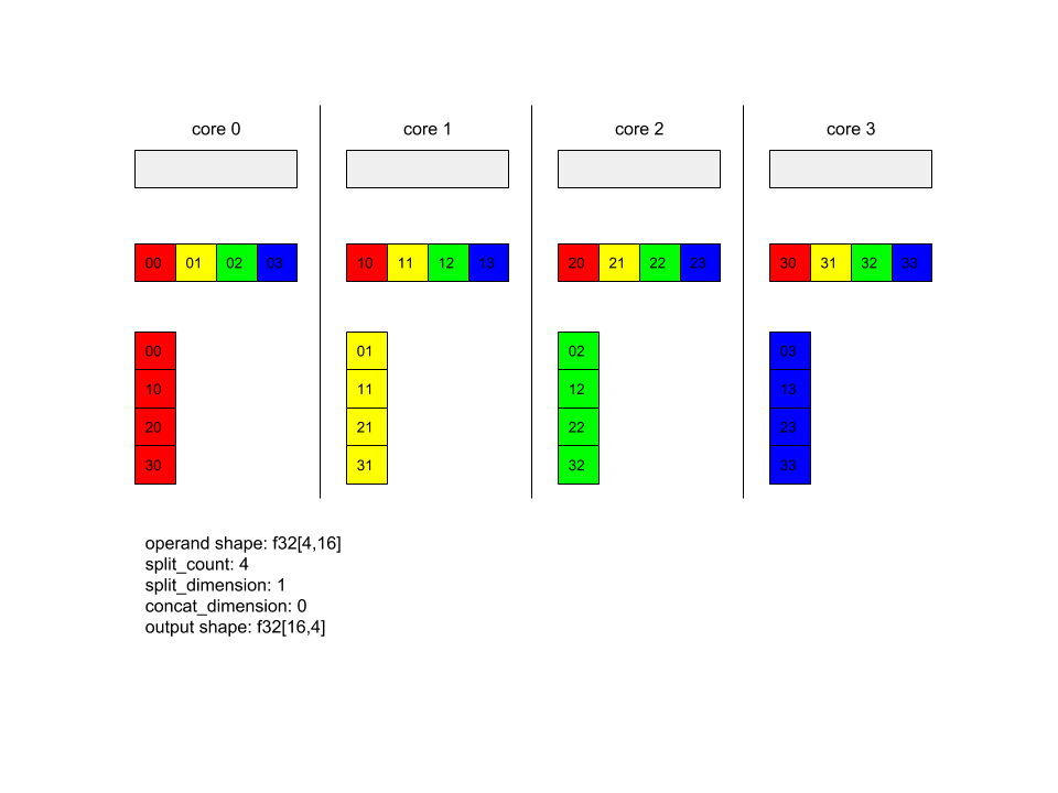
Dans cet exemple, quatre cœurs participent au modèle Alltoall. Sur chaque cœur, l'opérande est divisé en quatre parties le long de la dimension 0. Chaque partie a donc la forme f32[4,4]. Les quatre parties sont réparties sur tous les cœurs. Chaque cœur concatène ensuite les parties reçues selon la dimension 1, dans l'ordre des cœurs 0-4. La sortie de chaque cœur a donc la forme f32[16,4].
BatchNormGrad
Consultez également XlaBuilder::BatchNormGrad et l'article sur la normalisation des lots d'origine pour obtenir une description détaillée de l'algorithme.
Calcule les gradients d'une norme de lot.
BatchNormGrad(operand, scale, mean, variance, grad_output, epsilon, feature_index)
| Arguments | Type | Sémantique |
|---|---|---|
operand |
XlaOp |
tableau à n dimensions à normaliser (x) |
scale |
XlaOp |
Tableau à une dimension (\(\gamma\)) |
mean |
XlaOp |
Tableau à une dimension (\(\mu\)) |
variance |
XlaOp |
Tableau à une dimension (\(\sigma^2\)) |
grad_output |
XlaOp |
Gradients transmis à BatchNormTraining (\(\nabla y\)) |
epsilon |
float |
Valeur d'essilon (\(\epsilon\)) |
feature_index |
int64 |
Indice de la dimension de caractéristique dans operand |
Pour chaque caractéristique de la dimension de caractéristique (feature_index est l'index de la dimension d'élément géographique dans operand), l'opération calcule les dégradés par rapport à operand, offset et scale pour toutes les autres dimensions. feature_index doit être un index valide pour la dimension de caractéristique dans operand.
Les trois dégradés sont définis par les formules suivantes (en supposant qu'un tableau à quatre dimensions soit operand et que l'indice de dimension des caractéristiques soit l, la taille de lot m, et les tailles spatiales w et h):
\[ \begin{split} c_l&= \frac{1}{mwh}\sum_{i=1}^m\sum_{j=1}^w\sum_{k=1}^h \left( \nabla y_{ijkl} \frac{x_{ijkl} - \mu_l}{\sigma^2_l+\epsilon} \right) \\\\ d_l&= \frac{1}{mwh}\sum_{i=1}^m\sum_{j=1}^w\sum_{k=1}^h \nabla y_{ijkl} \\\\ \nabla x_{ijkl} &= \frac{\gamma_{l} }{\sqrt{\sigma^2_{l}+\epsilon} } \left( \nabla y_{ijkl} - d_l - c_l (x_{ijkl} - \mu_{l}) \right) \\\\ \nabla \gamma_l &= \sum_{i=1}^m\sum_{j=1}^w\sum_{k=1}^h \left( \nabla y_{ijkl} \frac{x_{ijkl} - \mu_l}{\sqrt{\sigma^2_{l}+\epsilon} } \right) \\\\\ \nabla \beta_l &= \sum_{i=1}^m\sum_{j=1}^w\sum_{k=1}^h \nabla y_{ijkl} \end{split} \]
Les entrées mean et variance représentent les valeurs de moment pour les dimensions de lot et spatiales.
Le type de sortie est un tuple de trois poignées:
| Sorties | Type | Sémantique |
|---|---|---|
grad_operand
|
XlaOp
|
dégradé par rapport à l'entrée operand ($\nabla
x$) |
grad_scale
|
XlaOp
|
gradient par rapport à l'entrée scale ($\nabla \gamma$) |
grad_offset
|
XlaOp
|
dégradé par rapport à l'entrée offset($\nabla
\beta$) |
BatchNormInference
Consultez également XlaBuilder::BatchNormInference et l'article sur la normalisation des lots d'origine pour obtenir une description détaillée de l'algorithme.
Normalise un tableau pour des dimensions de lot et spatiales.
BatchNormInference(operand, scale, offset, mean, variance, epsilon, feature_index)
| Arguments | Type | Sémantique |
|---|---|---|
operand |
XlaOp |
tableau à n dimensions à normaliser |
scale |
XlaOp |
Tableau à une dimension |
offset |
XlaOp |
Tableau à une dimension |
mean |
XlaOp |
Tableau à une dimension |
variance |
XlaOp |
Tableau à une dimension |
epsilon |
float |
Valeur d'Epsilon |
feature_index |
int64 |
Indice de la dimension de caractéristique dans operand |
Pour chaque caractéristique de la dimension de caractéristique (feature_index est l'indice de la dimension de caractéristique dans operand), l'opération calcule la moyenne et la variance pour toutes les autres dimensions, et utilise la moyenne et la variance pour normaliser chaque élément dans operand. feature_index doit être un index valide pour la dimension de caractéristique dans operand.
BatchNormInference équivaut à appeler BatchNormTraining sans calculer mean et variance pour chaque lot. Elle utilise à la place les valeurs estimées mean et variance. L'objectif de cette opération est de réduire la latence d'inférence, d'où le nom BatchNormInference.
La sortie est un tableau normalisé à N dimensions ayant la même forme que la valeur operand d'entrée.
BatchNormTraining
Consultez également XlaBuilder::BatchNormTraining et the original batch normalization paper pour obtenir une description détaillée de l'algorithme.
Normalise un tableau pour des dimensions de lot et spatiales.
BatchNormTraining(operand, scale, offset, epsilon, feature_index)
| Arguments | Type | Sémantique |
|---|---|---|
operand |
XlaOp |
tableau à n dimensions à normaliser (x) |
scale |
XlaOp |
Tableau à une dimension (\(\gamma\)) |
offset |
XlaOp |
Tableau à une dimension (\(\beta\)) |
epsilon |
float |
Valeur d'essilon (\(\epsilon\)) |
feature_index |
int64 |
Indice de la dimension de caractéristique dans operand |
Pour chaque caractéristique de la dimension de caractéristique (feature_index est l'indice de la dimension de caractéristique dans operand), l'opération calcule la moyenne et la variance pour toutes les autres dimensions, et utilise la moyenne et la variance pour normaliser chaque élément dans operand. feature_index doit être un index valide pour la dimension de caractéristique dans operand.
Pour chaque lot de operand \(x\) contenant des éléments m avec w et h comme taille de dimensions spatiales (en supposant que operand soit un tableau à 4 dimensions):
Calcule la moyenne par lot \(\mu_l\) pour chaque caractéristique
ldans la dimension de caractéristique : \(\mu_l=\frac{1}{mwh}\sum_{i=1}^m\sum_{j=1}^w\sum_{k=1}^h x_{ijkl}\)Calcule la variance de lot \(\sigma^2_l\): $\sigma^2l=\frac{1}{mwh}\sum{i=1}^m\sum{j=1}^w\sum{k=1}^h (x_{ijkl} - \mu_l)^2$
Normalise, met à l'échelle et décale : \(y_{ijkl}=\frac{\gamma_l(x_{ijkl}-\mu_l)}{\sqrt[2]{\sigma^2_l+\epsilon} }+\beta_l\)
La valeur epsilon, généralement un petit nombre, est ajoutée pour éviter les erreurs de division par zéro.
Le type de sortie est un tuple de trois XlaOp:
| Sorties | Type | Sémantique |
|---|---|---|
output
|
XlaOp
|
Tableau à n dimensions ayant la même forme que l'entrée operand (y) |
batch_mean |
XlaOp |
Tableau à une dimension (\(\mu\)) |
batch_var |
XlaOp |
Tableau à une dimension (\(\sigma^2\)) |
batch_mean et batch_var sont des moments calculés pour les dimensions de lot et spatiales à l'aide des formules ci-dessus.
BitcastConvertType
Consultez également XlaBuilder::BitcastConvertType.
Comme pour tf.bitcast dans TensorFlow, cette méthode effectue une opération de diffusion de bit au niveau de l'élément depuis une forme de données vers une forme cible. La taille d'entrée et de sortie doit correspondre: par exemple, les éléments s32 deviennent des éléments f32 via la routine Bitcast, et un élément s32 devient quatre éléments s8. Bitcast est implémenté en tant que cast de bas niveau. Par conséquent, les machines avec différentes représentations à virgule flottante génèrent des résultats différents.
BitcastConvertType(operand, new_element_type)
| Arguments | Type | Sémantique |
|---|---|---|
operand |
XlaOp |
tableau de type T avec les dièses D |
new_element_type |
PrimitiveType |
type U |
Les dimensions de l'opérande et de la forme cible doivent correspondre, à l'exception de la dernière dimension qui sera modifiée par le ratio de la taille de la primitive avant et après la conversion.
Les types d'éléments source et de destination ne doivent pas être des tuples.
Conversion de bitmap vers un type primitif de largeur différente
L'instruction HLO de BitcastConvert est compatible avec les cas où la taille du type d'élément de sortie T' n'est pas égale à celle de l'élément d'entrée T. Étant donné que, conceptuellement, l'opération est un bitcast et ne modifie pas les octets sous-jacents, la forme de l'élément de sortie doit changer. Pour B = sizeof(T), B' =
sizeof(T'), deux cas sont possibles.
Tout d'abord, lorsque la valeur est B > B', la forme de sortie obtient une nouvelle dimension mineure de taille B/B'. Exemple :
f16[10,2]{1,0} %output = f16[10,2]{1,0} bitcast-convert(f32[10]{0} %input)
La règle reste la même pour les scalaires efficaces:
f16[2]{0} %output = f16[2]{0} bitcast-convert(f32[] %input)
Pour B' > B, l'instruction nécessite également que la dernière dimension logique de la forme d'entrée soit égale à B'/B. Cette dimension est supprimée lors de la conversion:
f32[10]{0} %output = f32[10]{0} bitcast-convert(f16[10,2]{1,0} %input)
Notez que les conversions entre différentes largeurs de bits ne sont pas définies par éléments.
Diffusion
Consultez également XlaBuilder::Broadcast.
Ajoute des dimensions à un tableau en dupliquant les données dans le tableau.
Broadcast(operand, broadcast_sizes)
| Arguments | Type | Sémantique |
|---|---|---|
operand |
XlaOp |
Tableau à dupliquer |
broadcast_sizes |
ArraySlice<int64> |
Les tailles des nouvelles dimensions |
Les nouvelles dimensions sont insérées à gauche. Autrement dit, si broadcast_sizes a les valeurs {a0, ..., aN} et que la forme de l'opérande a les dimensions {b0, ..., bM}, la forme de la sortie a les dimensions {a0, ..., aN, b0, ..., bM}.
Le nouvel index de dimensions dans les copies de l'opérande, c'est-à-dire
output[i0, ..., iN, j0, ..., jM] = operand[j0, ..., jM]
Par exemple, si operand est un f32 scalaire avec la valeur 2.0f et que broadcast_sizes est {2, 3}, le résultat sera un tableau avec la forme f32[2, 3] et toutes les valeurs du résultat seront 2.0f.
BroadcastInDim
Consultez également XlaBuilder::BroadcastInDim.
Développe la taille et le rang d'un tableau en dupliquant les données qu'il contient.
BroadcastInDim(operand, out_dim_size, broadcast_dimensions)
| Arguments | Type | Sémantique |
|---|---|---|
operand |
XlaOp |
Tableau à dupliquer |
out_dim_size |
ArraySlice<int64> |
Les tailles des dimensions de la forme cible |
broadcast_dimensions |
ArraySlice<int64> |
À quelle dimension de la forme cible correspond chaque dimension de la forme de l'opérande |
Semblable à Broadcast, mais permet d'ajouter des dimensions n'importe où et d'étendre des dimensions existantes de taille 1.
Le operand est diffusé sous la forme décrite par out_dim_size.
broadcast_dimensions mappe les dimensions de operand aux dimensions de la forme cible, c'est-à-dire que la dimension "i" de l'opérande est mappée à la dimension "broadcast_dimension[i]" de la forme de sortie. Les dimensions de operand doivent avoir une taille 1 ou être identique à celle de la forme de sortie avec laquelle elles sont mappées. Les dimensions restantes sont renseignées par des dimensions de taille 1. La diffusion de dimensions dégénérées est ensuite diffusée le long de ces dimensions dégénérées pour atteindre la forme de sortie. La sémantique est décrite en détail sur la page Diffusion.
Call
Consultez également XlaBuilder::Call.
Invoque un calcul avec les arguments indiqués.
Call(computation, args...)
| Arguments | Type | Sémantique |
|---|---|---|
computation |
XlaComputation |
un calcul de type T_0, T_1, ..., T_{N-1} -> S avec N paramètres de type arbitraire |
args |
séquence de N XlaOp |
N arguments de type arbitraire |
L'arité et les types de args doivent correspondre aux paramètres de computation. Il n'est pas autorisé à avoir du args.
Cholesky
Consultez également XlaBuilder::Cholesky.
Calcule la décomposition de Cholésky d'un lot de matrices définies positives symétriques (hermitiennes).
Cholesky(a, lower)
| Arguments | Type | Sémantique |
|---|---|---|
a |
XlaOp |
un rang > 2 tableau d'un type complexe ou à virgule flottante. |
lower |
bool |
choisir d'utiliser le triangle supérieur ou inférieur de a. |
Si lower est true, calcule les matrices triangulaires inférieures l de sorte que $a = l .
l^T$. Si lower est false, calcule les matrices triangulaires supérieures u de sorte que\(a = u^T . u\).
Les données d'entrée sont lues uniquement à partir du triangle inférieur/supérieur de a, en fonction de la valeur de lower. Les valeurs de l'autre triangle sont ignorées. Les données de sortie sont renvoyées dans le même triangle. Les valeurs de l'autre triangle sont définies par l'implémentation et peuvent être n'importe quoi.
Si le rang de a est supérieur à 2, a est traité comme un lot de matrices, où toutes les dimensions, à l'exception des deux mineures, sont des dimensions de lot.
Si a n'est pas défini d'une valeur positive symétrique (hermite), le résultat est défini par l'implémentation.
Pince
Consultez également XlaBuilder::Clamp.
Fixe un opérande dans la plage comprise entre une valeur minimale et une valeur maximale.
Clamp(min, operand, max)
| Arguments | Type | Sémantique |
|---|---|---|
min |
XlaOp |
tableau de type T |
operand |
XlaOp |
tableau de type T |
max |
XlaOp |
tableau de type T |
Avec un opérande et des valeurs minimale et maximale, renvoie l'opérande s'il se trouve dans la plage comprise entre le minimum et le maximum, sinon renvoie la valeur minimale si l'opérande se trouve en dessous de cette plage ou la valeur maximale si l'opérande se trouve au-dessus de cette plage. Par exemple, clamp(a, x, b) = min(max(a, x), b).
Les trois tableaux doivent avoir la même forme. En tant que forme restreinte de diffusion, min et/ou max peuvent être une valeur scalaire de type T.
Exemple avec des valeurs scalaires min et max:
let operand: s32[3] = {-1, 5, 9};
let min: s32 = 0;
let max: s32 = 6;
==>
Clamp(min, operand, max) = s32[3]{0, 5, 6};
Réduire
Consultez également XlaBuilder::Collapse et l'opération tf.reshape.
Réduit les dimensions d'un tableau en une seule dimension.
Collapse(operand, dimensions)
| Arguments | Type | Sémantique |
|---|---|---|
operand |
XlaOp |
tableau de type T |
dimensions |
Vecteur int64 |
dans l'ordre et consécutif des dimensions de T. |
Le repli remplace le sous-ensemble donné de dimensions de l'opérande par une seule dimension. Les arguments d'entrée sont un tableau arbitraire de type T et un vecteur constant d'indices de dimension à la compilation. Les index de dimension doivent être un sous-ensemble consécutif de dimensions de T (dans l'ordre (nombres de dimensions croissants). Ainsi, {0, 1, 2}, {0, 1} ou {1, 2} sont tous des ensembles de dimensions valides, mais {1, 0} ou {0, 2} ne le sont pas. Elles sont remplacées par une seule nouvelle dimension, à la même position dans la séquence de dimensions que celles qu'elles remplacent, par la nouvelle taille de dimension égale au produit des tailles d'origine. Le nombre de dimension le plus bas dans dimensions correspond à la dimension la plus lente (la plus majeure) dans l'imbrication de boucle, qui réduit ces dimensions. Le nombre de dimension le plus élevé varie le plus (les plus faibles). Reportez-vous à l'opérateur tf.reshape si un ordre de réduction plus général est nécessaire.
Par exemple, supposons que "v" soit un tableau de 24 éléments:
let v = f32[4x2x3] { { {10, 11, 12},  {15, 16, 17} },
{ {20, 21, 22},  {25, 26, 27} },
{ {30, 31, 32},  {35, 36, 37} },
{ {40, 41, 42},  {45, 46, 47} } };

// Collapse to a single dimension, leaving one dimension.
let v012 = Collapse(v, {0,1,2});
then v012 == f32[24] {10, 11, 12, 15, 16, 17,
20, 21, 22, 25, 26, 27,
30, 31, 32, 35, 36, 37,
40, 41, 42, 45, 46, 47};

// Collapse the two lower dimensions, leaving two dimensions.
let v01 = Collapse(v, {0,1});
then v01 == f32[4x6] { {10, 11, 12, 15, 16, 17},
{20, 21, 22, 25, 26, 27},
{30, 31, 32, 35, 36, 37},
{40, 41, 42, 45, 46, 47} };

// Collapse the two higher dimensions, leaving two dimensions.
let v12 = Collapse(v, {1,2});
then v12 == f32[8x3] { {10, 11, 12},
{15, 16, 17},
{20, 21, 22},
{25, 26, 27},
{30, 31, 32},
{35, 36, 37},
{40, 41, 42},
{45, 46, 47} };
CollectivePermute
Consultez également XlaBuilder::CollectivePermute.
CollectivePermute est une opération collective qui envoie et reçoit des instances répliquées de données.
CollectivePermute(operand, source_target_pairs)
| Arguments | Type | Sémantique |
|---|---|---|
operand |
XlaOp |
Tableau d'entrée à n dimensions |
source_target_pairs |
Vecteur <int64, int64> |
Une liste des paires (source_Replica_id, target_répli_id). Pour chaque paire, l'opérande est envoyé de l'instance répliquée source à l'instance répliquée cible. |
Notez que les restrictions suivantes s'appliquent à source_target_pair:
- Deux paires ne doivent pas avoir le même ID d'instance répliquée cible ni le même ID d'instance répliquée source.
- Si un ID d'instance répliquée n'est une cible dans aucune paire, la sortie de cette instance répliquée est un Tensor composé de zéro(s) ayant la même forme que l'entrée.
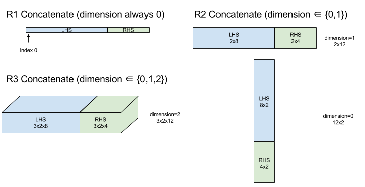
Concatenate
Consultez également XlaBuilder::ConcatInDim.
Concaténer compose un tableau à partir de plusieurs opérandes de tableau. Le tableau a le même rang que chacun des opérandes du tableau d'entrée (qui doivent avoir le même rang) et contient les arguments dans l'ordre dans lequel ils ont été spécifiés.
Concatenate(operands..., dimension)
| Arguments | Type | Sémantique |
|---|---|---|
operands |
séquence de N XlaOp |
N tableaux de type T avec les dimensions [L0, L1, ...]. Nécessite N >= 1. |
dimension |
int64 |
Valeur de l'intervalle [0, N) qui nomme la dimension à concaténer entre les operands. |
Toutes les dimensions doivent être identiques, à l'exception de dimension. En effet, XLA n'est pas compatible avec les tableaux "irréguliers". Notez également que les valeurs "rank-0" ne peuvent pas être concaténées (car il est impossible de nommer la dimension associée à la concaténation).
Exemple unidimensionnel:
Concat({ {2, 3}, {4, 5}, {6, 7} }, 0)
>>> {2, 3, 4, 5, 6, 7}
Exemple en deux dimensions:
let a = {
{1, 2},
{3, 4},
{5, 6},
};
let b = {
{7, 8},
};
Concat({a, b}, 0)
>>> {
{1, 2},
{3, 4},
{5, 6},
{7, 8},
}
Schéma:
Conditional
Consultez également XlaBuilder::Conditional.
Conditional(pred, true_operand, true_computation, false_operand,
false_computation)
| Arguments | Type | Sémantique |
|---|---|---|
pred |
XlaOp |
Scalaire de type PRED |
true_operand |
XlaOp |
Argument de type \(T_0\) |
true_computation |
XlaComputation |
XlaComputation de type \(T_0 \to S\) |
false_operand |
XlaOp |
Argument de type \(T_1\) |
false_computation |
XlaComputation |
XlaComputation de type \(T_1 \to S\) |
Exécute true_computation si pred est défini sur true, false_computation si pred est false, et renvoie le résultat.
La méthode true_computation doit utiliser un seul argument de type \(T_0\) et sera appelée avec true_operand, qui doit être du même type. L'élément false_computation doit accepter un seul argument de type \(T_1\) et sera appelé avec false_operand, qui doit être du même type. Le type de la valeur renvoyée pour true_computation et false_computation doit être identique.
Notez que seul true_computation et false_computation sera exécuté en fonction de la valeur de pred.
Conditional(branch_index, branch_computations, branch_operands)
| Arguments | Type | Sémantique |
|---|---|---|
branch_index |
XlaOp |
Scalaire de type S32 |
branch_computations |
séquence de N XlaComputation |
XlaComputations de type \(T_0 \to S , T_1 \to S , ..., T_{N-1} \to S\) |
branch_operands |
séquence de N XlaOp |
Arguments de type \(T_0 , T_1 , ..., T_{N-1}\) |
Exécute branch_computations[branch_index] et renvoie le résultat. Si branch_index est une S32 inférieure à 0 ou >= N, branch_computations[N-1] est exécuté comme branche par défaut.
Chaque branch_computations[b] doit contenir un seul argument de type \(T_b\) et sera appelé avec branch_operands[b], qui doit être du même type. Le type de la valeur renvoyée de chaque branch_computations[b] doit être le même.
Notez qu'un seul des branch_computations sera exécuté en fonction de la valeur de branch_index.
Conv. (convolution)
Consultez également XlaBuilder::Conv.
En tant que ConvWithGeneralPadding, mais la marge intérieure est spécifiée de manière abrégée comme étant MÊME ou VALIDE. La MÊME marge intérieure remplit l'entrée (lhs) avec des zéros pour que la sortie ait la même forme que l'entrée lorsqu'elle n'est pas prise en compte. Un remplissage VALIDE signifie simplement pas de marge intérieure.
ConvWithGeneralPadding (convolution)
Consultez également XlaBuilder::ConvWithGeneralPadding.
Calcule une convolution du type utilisé dans les réseaux de neurones. Ici, une convolution peut être considérée comme une fenêtre à N dimensions se déplaçant sur une zone de base à N dimensions, et un calcul est effectué pour chaque position possible de la fenêtre.
| Arguments | Type | Sémantique |
|---|---|---|
lhs |
XlaOp |
classement n+2 tableau d'entrées |
rhs |
XlaOp |
rang n+2 tableau des pondérations de noyau |
window_strides |
ArraySlice<int64> |
Tableau n-d de pas de noyau |
padding |
ArraySlice< pair<int64,int64>> |
Tableau n-d de marge intérieure (faible, élevée) |
lhs_dilation |
ArraySlice<int64> |
Tableau de facteurs de dilation n-d lhs |
rhs_dilation |
ArraySlice<int64> |
Tableau de facteurs de dilation n-d rhs |
feature_group_count |
int64 | le nombre de groupes de caractéristiques |
batch_group_count |
int64 | le nombre de groupes de lots |
Soit n le nombre de dimensions spatiales. L'argument lhs est un tableau de rang n+2 décrivant l'aire de base. C'est ce qu'on appelle l'entrée, même si
bien sûr le rhs est aussi une entrée. Dans un réseau de neurones, il s'agit des activations d'entrée.
Les dimensions n+2 sont, dans cet ordre:
batch: chaque coordonnée de cette dimension représente une entrée indépendante pour laquelle une convolution est effectuée.z/depth/features: chaque position (y,x) dans l'aire de base est associée à un vecteur, qui entre dans cette dimension.spatial_dims: décrit les dimensions spatialesnqui définissent la zone de base sur laquelle la fenêtre se déplace.
L'argument rhs est un tableau de rang n+2 décrivant le filtre/noyau/fenêtre de convolution. Les dimensions sont les suivantes, dans cet ordre:
output-z: dimensionzde la sortie.input-z: la taille de cette dimension multipliée parfeature_group_countdoit être égale à la taille de la dimensionzen lhs.spatial_dims: décrit les dimensions spatialesnqui définissent la fenêtre n-d qui se déplace dans la zone de base.
L'argument window_strides spécifie le pas de la fenêtre convolutive dans les dimensions spatiales. Par exemple, si le pas de la première dimension spatiale est de 3, la fenêtre ne peut être placée qu'aux coordonnées où le premier index spatial est divisible par 3.
L'argument padding spécifie la quantité de marge intérieure nulle à appliquer à la zone de base. La quantité de marge intérieure peut être négative. La valeur absolue de la marge intérieure négative indique le nombre d'éléments à supprimer de la dimension spécifiée avant d'effectuer la convolution. padding[0] spécifie la marge intérieure pour la dimension y et padding[1] spécifie la marge intérieure pour la dimension x. Chaque paire a la marge intérieure la plus faible comme premier élément et la marge intérieure élevée comme deuxième élément. La marge intérieure inférieure est appliquée dans la direction des indices inférieurs, tandis que la marge intérieure élevée est appliquée dans la direction des indices plus élevés. Par exemple, si padding[1] correspond à (2,3), il y aura une marge intérieure de 2 zéros à gauche et de 3 zéros à droite dans la deuxième dimension spatiale. L'utilisation du remplissage équivaut à insérer ces mêmes valeurs nulles dans l'entrée (lhs) avant d'effectuer la convolution.
Les arguments lhs_dilation et rhs_dilation spécifient le facteur de dilation à appliquer respectivement aux valeurs lhs et rhs dans chaque dimension spatiale. Si le facteur de dilation dans une dimension spatiale est "d", alors les trous d-1 sont implicitement placés entre chacune des entrées de cette dimension, augmentant ainsi la taille du tableau. Les trous sont remplis avec une valeur "no-op", ce qui correspond à des zéros pour la convolution.
La dilatation des rhéses est également appelée convolution atrus. Pour en savoir plus, consultez tf.nn.atrous_conv2d. La dilation du lhs est également appelée convolution transposée. Pour en savoir plus, consultez tf.nn.conv2d_transpose.
L'argument feature_group_count (valeur par défaut 1) peut être utilisé pour les convolutions groupées. feature_group_count doit être un diviseur de la dimension de caractéristique d'entrée et de sortie. Si feature_group_count est supérieur à 1, cela signifie que, conceptuellement, la dimension de caractéristique d'entrée et de sortie et la dimension de caractéristique de sortie rhs sont divisées équitablement en plusieurs groupes feature_group_count, chacun étant constitué d'une sous-séquence consécutive de caractéristiques. La dimension de caractéristique d'entrée de rhs doit être égale à la dimension de caractéristique d'entrée lhs divisée par feature_group_count (elle a donc déjà la taille d'un groupe de caractéristiques d'entrée). Les i-ièmes groupes sont utilisés ensemble pour calculer feature_group_count pour de nombreuses convolutions distinctes. Les résultats de ces convolutions sont concaténés dans la dimension de caractéristique de sortie.
Pour une convolution en profondeur, l'argument feature_group_count serait défini sur la dimension de caractéristique d'entrée, et le filtre passerait de [filter_height, filter_width, in_channels, channel_multiplier] à [filter_height, filter_width, 1, in_channels * channel_multiplier]. Pour en savoir plus, consultez tf.nn.depthwise_conv2d.
L'argument batch_group_count (valeur par défaut 1) peut être utilisé pour les filtres groupés lors de la rétropropagation. batch_group_count doit être un diviseur de la taille de la dimension de lot lhs (entrée). Si batch_group_count est supérieur à 1, cela signifie que la dimension du lot de sortie doit avoir la taille input batch
/ batch_group_count. batch_group_count doit être un diviseur de la taille de l'élément géographique de sortie.
La forme de sortie présente les dimensions suivantes, dans l'ordre suivant:
batch: la taille de cette dimension multipliée parbatch_group_countdoit être égale à la taille de la dimensionbatchen lhs.z: même taille queoutput-zsur le noyau (rhs).spatial_dims: une valeur pour chaque emplacement valide de la fenêtre convolutive.

La figure ci-dessus montre le fonctionnement du champ batch_group_count. En réalité, nous divisons chaque lot LH en groupes batch_group_count, et nous faisons de même pour les caractéristiques de sortie. Ensuite, pour chacun de ces groupes, nous effectuons des convolutions par paire, puis nous concaténons la sortie avec la dimension de caractéristique de sortie. La sémantique opérationnelle de toutes les autres dimensions (caractéristique et spatiale) reste la même.
Les emplacements valides de la fenêtre convolutive sont déterminés par les progrès et la taille de la zone de base après la marge intérieure.
Pour décrire ce qu'une convolution fait, considérez une convolution 2D et choisissez des coordonnées batch, z, y et x fixes dans la sortie. Ensuite, (y,x) est la position d'un angle de la fenêtre dans la zone de la base (par exemple, le coin supérieur gauche, en fonction de la manière dont vous interprétez les dimensions spatiales). Nous avons maintenant une fenêtre 2D, prise à partir de l'aire de la base, où chaque point 2D est associé à un vecteur 1d, nous obtenons donc une boîte 3D. À partir du noyau convolutif, comme nous avons corrigé la coordonnée de sortie z, nous disposons également d'une zone 3D. Les deux cases ont les mêmes dimensions. Nous pouvons donc prendre la somme des produits par élément entre les deux cases (semblable à un produit scalaire). Il s'agit de la valeur de sortie.
Notez que si output-z est, par exemple, 5, chaque position de la fenêtre génère 5 valeurs dans la sortie dans la dimension z de la sortie. Ces valeurs diffèrent selon la partie du noyau convolutif utilisée. Un cadre de valeurs 3D distinct est utilisé pour chaque coordonnée output-z. Vous pouvez donc considérer cela comme cinq convolutions distinctes avec un filtre différent pour chacune d'elles.
Voici un pseudo-code pour une convolution 2D avec marge intérieure et progression:
for (b, oz, oy, ox) {  // output coordinates
  value = 0;
  for (iz, ky, kx) {  // kernel coordinates and input z
    iy = oy*stride_y + ky - pad_low_y;
    ix = ox*stride_x + kx - pad_low_x;
    if ((iy, ix) inside the base area considered without padding) {
      value += input(b, iz, iy, ix) * kernel(oz, iz, ky, kx);
    }
  }
  output(b, oz, oy, ox) = value;
}
ConvertElementType
Consultez également XlaBuilder::ConvertElementType.
À l'instar d'une static_cast au niveau d'un élément en C++, cette méthode effectue une opération de conversion par élément d'une forme de données à une forme cible. Les dimensions doivent correspondre, et la conversion doit être effectuée au niveau des éléments. Par exemple, les éléments s32 deviennent des éléments f32 via une routine de conversion s32 en f32.
ConvertElementType(operand, new_element_type)
| Arguments | Type | Sémantique |
|---|---|---|
operand |
XlaOp |
tableau de type T avec les dièses D |
new_element_type |
PrimitiveType |
type U |
Les dimensions de l'opérande et de la forme cible doivent correspondre. Les types d'éléments source et de destination ne doivent pas être des tuples.
Une conversion telle que T=s32 en U=f32 exécutera une routine de conversion de normalisation de type "int-to-float", telle que "round-to-qua-est-even".
let a: s32[3] = {0, 1, 2};
let b: f32[3] = convert(a, f32);
then b == f32[3]{0.0, 1.0, 2.0}
CrossReplicaSum
Exécute AllReduce avec un calcul de somme.
CustomCall
Consultez également XlaBuilder::CustomCall.
Appeler une fonction fournie par l'utilisateur dans un calcul.
CustomCall(target_name, args..., shape)
| Arguments | Type | Sémantique |
|---|---|---|
target_name |
string |
Nom de la fonction. Une instruction d'appel ciblant ce nom de symbole sera émise. |
args |
séquence de N XlaOp |
N arguments de type arbitraire, qui seront transmis à la fonction. |
shape |
Shape |
Forme de sortie de la fonction |
La signature de la fonction est identique, quels que soient l'arité ou le type d'arguments:
extern "C" void target_name(void* out, void** in);
Par exemple, si la fonctionnalité d'appel personnalisé est utilisée comme suit:
let x = f32[2] {1,2};
let y = f32[2x3] { {10, 20, 30}, {40, 50, 60} };

CustomCall("myfunc", {x, y}, f32[3x3])
Voici un exemple d'implémentation de myfunc:
extern "C" void myfunc(void* out, void** in) {
  float (&x)[2] = *static_cast<float(*)[2]>(in[0]);
  float (&y)[2][3] = *static_cast<float(*)[2][3]>(in[1]);
  EXPECT_EQ(1, x[0]);
  EXPECT_EQ(2, x[1]);
  EXPECT_EQ(10, y[0][0]);
  EXPECT_EQ(20, y[0][1]);
  EXPECT_EQ(30, y[0][2]);
  EXPECT_EQ(40, y[1][0]);
  EXPECT_EQ(50, y[1][1]);
  EXPECT_EQ(60, y[1][2]);
  float (&z)[3][3] = *static_cast<float(*)[3][3]>(out);
  z[0][0] = x[1] + y[1][0];
  // ...
}
La fonction fournie par l'utilisateur ne doit pas avoir d'effets secondaires et son exécution doit être idempotente.
Dot
Consultez également XlaBuilder::Dot.
Dot(lhs, rhs)
| Arguments | Type | Sémantique |
|---|---|---|
lhs |
XlaOp |
tableau de type T |
rhs |
XlaOp |
tableau de type T |
La sémantique exacte de cette opération dépend des rangs des opérandes:
| Entrée | Sortie | Sémantique |
|---|---|---|
vecteur [n] dot vecteur [n] |
scalaire | produit scalaire vectoriel |
matrice [m x k] vecteur dot [k] |
vecteur [m] | multiplication matricielle-vecteur |
matrice [m x k] matrice dot [k x k] |
matrice [m x n] | multiplication matrice-matrice |
L'opération effectue la somme des produits pour la deuxième dimension de lhs (ou la première si elle est de rang 1) et la première dimension de rhs. Ce sont les dimensions "contractées". Les dimensions contractées de lhs et rhs doivent être de la même taille. En pratique, il permet d'effectuer des produits scalaires entre des vecteurs, des multiplications de vecteur/matrice ou des multiplications matrice/matrice.
DotGeneral
Consultez également XlaBuilder::DotGeneral.
DotGeneral(lhs, rhs, dimension_numbers)
| Arguments | Type | Sémantique |
|---|---|---|
lhs |
XlaOp |
tableau de type T |
rhs |
XlaOp |
tableau de type T |
dimension_numbers |
DotDimensionNumbers |
les nombres de dimensions de lot et de contraction |
Semblable à Dot, mais permet de spécifier des numéros de dimension de contrat et de lot à la fois pour lhs et rhs.
| Champs DotDimensionNumbers | Type | Sémantique |
|---|---|---|
lhs_contracting_dimensions
|
(valeur répétée de type int64) | lhs numéros de dimension contractant |
rhs_contracting_dimensions
|
(valeur répétée de type int64) | rhs numéros de dimension contractant |
lhs_batch_dimensions
|
(valeur répétée de type int64) | lhs numéros de dimension de lot |
rhs_batch_dimensions
|
(valeur répétée de type int64) | rhs numéros de dimension de lot |
DotGeneral effectue la somme des produits sur les dimensions contractantes spécifiées dans dimension_numbers.
Les numéros de dimensions contractées associées à partir de lhs et rhs n'ont pas besoin d'être identiques, mais doivent avoir les mêmes dimensions.
Exemple avec des numéros de dimension contractants:
lhs = { {1.0, 2.0, 3.0},
{4.0, 5.0, 6.0} }

rhs = { {1.0, 1.0, 1.0},
{2.0, 2.0, 2.0} }

DotDimensionNumbers dnums;
dnums.add_lhs_contracting_dimensions(1);
dnums.add_rhs_contracting_dimensions(1);

DotGeneral(lhs, rhs, dnums) -> { {6.0, 12.0},
{15.0, 30.0} }
Les numéros de dimension de lot associés à partir de lhs et rhs doivent avoir les mêmes tailles de dimension.
Exemple avec des nombres de dimension de lot (taille de lot 2, matrices 2x2):
lhs = { { {1.0, 2.0},
{3.0, 4.0} },
{ {5.0, 6.0},
{7.0, 8.0} } }

rhs = { { {1.0, 0.0},
{0.0, 1.0} },
{ {1.0, 0.0},
{0.0, 1.0} } }

DotDimensionNumbers dnums;
dnums.add_lhs_contracting_dimensions(2);
dnums.add_rhs_contracting_dimensions(1);
dnums.add_lhs_batch_dimensions(0);
dnums.add_rhs_batch_dimensions(0);

DotGeneral(lhs, rhs, dnums) -> { { {1.0, 2.0},
{3.0, 4.0} },
{ {5.0, 6.0},
{7.0, 8.0} } }
| Entrée | Sortie | Sémantique |
|---|---|---|
[b0, m, k] dot [b0, k, n] |
[b0, m, n] | matmul par lot |
[b0, b1, m, k] dot [b0, b1, k, n] |
[b0, b1, m, n] | matmul par lot |
Il s'ensuit que le numéro de dimension résultant commence par la dimension de lot, puis la dimension lhs non contractuelle, non liée au lot, et enfin la dimension rhs non contractuelle.
DynamicSlice
Consultez également XlaBuilder::DynamicSlice.
DynamicSlice extrait un sous-tableau du tableau d'entrée au niveau du start_indices dynamique. La taille de la tranche dans chaque dimension est transmise dans size_indices, qui spécifie le point de fin des intervalles de secteurs exclusifs dans chaque dimension: [début, début + taille). La forme de start_indices doit être un rang ==
1, la taille de la dimension doit être égale au rang de operand.
DynamicSlice(operand, start_indices, size_indices)
| Arguments | Type | Sémantique |
|---|---|---|
operand |
XlaOp |
Tableau à N dimensions de type T |
start_indices |
séquence de N XlaOp |
Liste des N entiers scalaires contenant les index de départ de la tranche pour chaque dimension. La valeur doit être supérieure ou égale à zéro. |
size_indices |
ArraySlice<int64> |
Liste de N entiers contenant la taille de tranche pour chaque dimension. Chaque valeur doit être strictement supérieure à zéro, et la combinaison début + taille doit être inférieure ou égale à la taille de la dimension pour éviter d'encapsuler la taille de la dimension modulo. |
Les index de tranche effective sont calculés en appliquant la transformation suivante pour chaque indice i dans [1, N) avant d'effectuer la tranche:
start_indices[i] = clamp(start_indices[i], 0, operand.dimension_size[i] - size_indices[i])
Cela garantit que la tranche extraite est toujours comprise dans les limites par rapport au tableau d'opérandes. Si la tranche est comprise dans les limites avant l'application de la transformation, celle-ci n'a aucun effet.
Exemple unidimensionnel:
let a = {0.0, 1.0, 2.0, 3.0, 4.0}
let s = {2}

DynamicSlice(a, s, {2}) produces:
{2.0, 3.0}
Exemple en deux dimensions:
let b =
{ {0.0,  1.0,  2.0},
{3.0,  4.0,  5.0},
{6.0,  7.0,  8.0},
{9.0, 10.0, 11.0} }
let s = {2, 1}

DynamicSlice(b, s, {2, 2}) produces:
{ { 7.0,  8.0},
{10.0, 11.0} }
DynamicUpdateSlice
Consultez également XlaBuilder::DynamicUpdateSlice.
DynamicUpdateSlice génère un résultat qui correspond à la valeur du tableau d'entrée operand, avec une tranche update remplacée par start_indices.
La forme de update détermine celle du sous-tableau du résultat mis à jour.
La forme de start_indices doit être un rang de 1, avec une taille de dimension égale au rang de operand.
DynamicUpdateSlice(operand, update, start_indices)
| Arguments | Type | Sémantique |
|---|---|---|
operand |
XlaOp |
Tableau à N dimensions de type T |
update |
XlaOp |
Tableau à N dimensions de type T contenant la mise à jour des tranches. Chaque dimension de la forme de mise à jour doit être strictement supérieure à zéro, et la valeur "début" et "mise à jour" doit être inférieure ou égale à la taille de l'opérande de chaque dimension afin d'éviter de générer des index de mise à jour hors limites. |
start_indices |
séquence de N XlaOp |
Liste des N entiers scalaires contenant les index de départ de la tranche pour chaque dimension. La valeur doit être supérieure ou égale à zéro. |
Les index de tranche effective sont calculés en appliquant la transformation suivante pour chaque indice i dans [1, N) avant d'effectuer la tranche:
start_indices[i] = clamp(start_indices[i], 0, operand.dimension_size[i] - update.dimension_size[i])
Cela garantit que la tranche mise à jour est toujours comprise dans les limites par rapport au tableau d'opérandes. Si la tranche est comprise dans les limites avant l'application de la transformation, celle-ci n'a aucun effet.
Exemple unidimensionnel:
let a = {0.0, 1.0, 2.0, 3.0, 4.0}
let u = {5.0, 6.0}
let s = {2}

DynamicUpdateSlice(a, u, s) produces:
{0.0, 1.0, 5.0, 6.0, 4.0}
Exemple en deux dimensions:
let b =
{ {0.0,  1.0,  2.0},
{3.0,  4.0,  5.0},
{6.0,  7.0,  8.0},
{9.0, 10.0, 11.0} }
let u =
{ {12.0,  13.0},
{14.0,  15.0},
{16.0,  17.0} }

let s = {1, 1}

DynamicUpdateSlice(b, u, s) produces:
{ {0.0,  1.0,  2.0},
{3.0, 12.0, 13.0},
{6.0, 14.0, 15.0},
{9.0, 16.0, 17.0} }
Opérations arithmétiques binaires par élément
Consultez également XlaBuilder::Add.
Un ensemble d'opérations arithmétiques binaires par élément est pris en charge.
Op(lhs, rhs)
Où Op est l'une des valeurs suivantes : Add (addition), Sub (soustraction), Mul (multiplication), Div (division), Rem (reste), Max (maximum), Min (minimum), LogicalAnd (opérateur logique AND) ou LogicalOr (opérateur logique OR).
| Arguments | Type | Sémantique |
|---|---|---|
lhs |
XlaOp |
Opérande de gauche: tableau de type T |
rhs |
XlaOp |
Opérande de droite: tableau de type T |
Les formes des arguments doivent être similaires ou compatibles. Consultez la documentation sur la diffusion pour découvrir comment les formes sont compatibles. Le résultat d'une opération présente une forme résultant de la diffusion des deux tableaux d'entrée. Dans cette variante, les opérations entre des tableaux de différents rangs ne sont pas acceptées, sauf si l'un des opérandes est scalaire.
Lorsque Op est défini sur Rem, le signe du résultat est tiré du dividende, et la valeur absolue du résultat est toujours inférieure à la valeur absolue du diviseur.
Un dépassement de division entier (division/reste signé/non signé par zéro ou division/reste signé de INT_SMIN avec -1) génère une valeur définie par l'implémentation.
Il existe une autre variante compatible avec la diffusion de rangs différents pour ces opérations:
Op(lhs, rhs, broadcast_dimensions)
Où Op est identique à ci-dessus. Cette variante de l'opération doit être utilisée pour les opérations arithmétiques entre des tableaux de rangs différents (par exemple, pour ajouter une matrice à un vecteur).
L'opérande broadcast_dimensions supplémentaire est une tranche d'entiers utilisée pour étendre le rang de l'opérande de rang inférieur au rang de l'opérande de rang supérieur. broadcast_dimensions mappe les dimensions de la forme de rang inférieur aux dimensions de la forme de rang supérieur. Les dimensions non mappées de la forme développée sont remplies avec des dimensions de taille un. Le broadcasting de dimension dégénérée diffuse ensuite les formes le long de ces dimensions dégénérées pour égaliser les formes des deux opérandes. La sémantique est décrite en détail sur la page Diffusion.
Opérations de comparaison par élément
Consultez également XlaBuilder::Eq.
Un ensemble d'opérations de comparaison binaire par élément standard est accepté. Notez que la sémantique de comparaison à virgule flottante de la norme IEEE 754 s'applique lors de la comparaison de types à virgule flottante.
Op(lhs, rhs)
Où Op est l'une des valeurs suivantes : Eq (égal à), Ne (pas égal à), Ge (supérieur ou égal à), Gt (supérieur à), Le (inférieur ou égal à), Lt (inférieur à). Un autre ensemble d'opérateurs, EqTotalOrder, NeTotalOrder, GeTotalOrder, GtTotalOrder, LeTotalOrder et LtTotalOrder, offrent les mêmes fonctionnalités, sauf qu'ils prennent en charge un ordre total sur les nombres à virgule flottante, en appliquant -NaN < -Inf < -Finite < -0 < +0 < +Infnite < +Infnite < +
| Arguments | Type | Sémantique |
|---|---|---|
lhs |
XlaOp |
Opérande de gauche: tableau de type T |
rhs |
XlaOp |
Opérande de droite: tableau de type T |
Les formes des arguments doivent être similaires ou compatibles. Consultez la documentation sur la diffusion pour découvrir comment les formes sont compatibles. Le résultat d'une opération présente une forme qui est le résultat de la diffusion des deux tableaux d'entrée avec le type d'élément PRED. Dans cette variante, les opérations entre des tableaux de rangs différents ne sont pas acceptées, sauf si l'un des opérandes est scalaire.
Il existe une autre variante compatible avec la diffusion de rangs différents pour ces opérations:
Op(lhs, rhs, broadcast_dimensions)
Où Op est identique à ci-dessus. Cette variante de l'opération doit être utilisée pour comparer des opérations entre des tableaux de rangs différents (par exemple, pour ajouter une matrice à un vecteur).
L'opérande broadcast_dimensions supplémentaire est une tranche d'entiers spécifiant les dimensions à utiliser pour diffuser les opérandes. La sémantique est décrite en détail sur la page Diffusion.
Fonctions unaires par élément
XlaBuilder prend en charge ces fonctions unaires par élément:
Abs(operand) x -> |x| d'absorption par élément par élément.
Ceil(operand) Seuil par élément x -> ⌈x⌉.
Cos(operand) Cosinus x -> cos(x) au niveau de l'élément.
Exp(operand) x -> e^x exponentielle naturel par élément.
Floor(operand) Étage x -> ⌊x⌋ par élément.
Imag(operand) Partie imaginaire par élément d'une forme complexe (ou réelle). x -> imag(x). Si l'opérande est de type à virgule flottante, renvoie 0.
IsFinite(operand) vérifie si chaque élément de operand est fini (c'est-à-dire s'il n'est pas infini positif ou négatif), et n'est pas NaN. Renvoie un tableau de valeurs PRED ayant la même forme que l'entrée, où chaque élément est true si et seulement si l'élément d'entrée correspondant est fini.
Log(operand) Logarithme naturel par élément x -> ln(x).
LogicalNot(operand) Logique par élément non x -> !(x).
Logistic(operand) Calcul de la fonction logistique par élément x ->
logistic(x).
PopulationCount(operand) Calcule le nombre de bits définis dans chaque élément de operand.
Neg(operand) Négation par élément x -> -x.
Real(operand) Partie réelle par élément d'une forme complexe (ou réelle).
x -> real(x). Si l'opérande est de type à virgule flottante, renvoie la même valeur.
Rsqrt(operand) Réciproque élément par élément de l'opération de racine carrée x -> 1.0 / sqrt(x).
Sign(operand) Opération de signature par élément x -> sgn(x) où
\[\text{sgn}(x) = \begin{cases} -1 & x < 0\\ -0 & x = -0\\ NaN & x = NaN\\ +0 & x = +0\\ 1 & x > 0 \end{cases}\]
à l'aide de l'opérateur de comparaison pour le type d'élément operand.
Sqrt(operand) Opération de racine carrée de l'élément x -> sqrt(x).
Cbrt(operand) Opération de racine cubique par élément x -> cbrt(x).
Tanh(operand) Tangente hyperbolique par élément x -> tanh(x).
Round(operand) Arrondi au niveau des éléments, écarte la valeur zéro.
RoundNearestEven(operand) Arrondi au niveau des éléments, correspond au pair le plus proche.
| Arguments | Type | Sémantique |
|---|---|---|
operand |
XlaOp |
L'opérande de la fonction |
La fonction est appliquée à chaque élément du tableau operand, ce qui génère un tableau ayant la même forme. operand peut être un scalaire (rang 0).
Fft
L'opération XLA FFT implémente les transformations de Fourier avant et inverse pour les entrées/sorties réelles et complexes. Les FFT multidimensionnels sont acceptés sur un maximum de trois axes.
Consultez également XlaBuilder::Fft.
| Arguments | Type | Sémantique |
|---|---|---|
operand |
XlaOp |
Tableau que nous transformons de Fourier. |
fft_type |
FftType |
Consultez le tableau ci-dessous. |
fft_length |
ArraySlice<int64> |
Longueurs du domaine temporel des axes transformés. Cela est particulièrement nécessaire pour qu'IRFFT puisse redimensionner l'axe le plus interne à droite, car RFFT(fft_length=[16]) a la même forme de sortie que RFFT(fft_length=[17]). |
FftType |
Sémantique |
|---|---|
FFT |
FFT complexe à complexe. La forme reste inchangée. |
IFFT |
FFT inverse de complexe à complexe. La forme reste inchangée. |
RFFT |
Transmission du vrai au complexe FFT. La forme de l'axe le plus interne est réduite à fft_length[-1] // 2 + 1 si fft_length[-1] est une valeur non nulle, en omettant la partie conjuguée inversée du signal transformé au-delà de la fréquence de Nyquist. |
IRFFT |
FFT inverse de vrai à complexe (en d'autres termes, prend complexe et renvoie des valeurs réelles). La forme de l'axe le plus interne est développée à fft_length[-1] si fft_length[-1] est une valeur non nulle, en déduisant la partie du signal transformé au-delà de la fréquence de Nyquist à partir du conjugué inverse des entrées 1 en fft_length[-1] // 2 + 1. |
FFT multidimensionnel
Lorsque plusieurs valeurs fft_length sont fournies, cela équivaut à appliquer une cascade d'opérations FFT à chacun des axes les plus internes. Notez que pour les cas réels, complexes et complexes, la transformation de l'axe le plus interne est (effectivement) effectuée en premier (RFFT, dernier pour IRFFT). C'est pourquoi l'axe le plus interne est celui qui modifie la taille. Les autres transformations d'axe seront alors complexes.
Détails de mise en œuvre
Le processeur FFT s'appuie sur TensorFFT d'Eigen. FFT GPU utilise cuFFT.
Rassembler
L'opération de collecte XLA assemble plusieurs tranches d'un tableau d'entrée (chaque tranche à un décalage d'exécution potentiellement différent).
Sémantique générale
Consultez également XlaBuilder::Gather.
Pour une description plus intuitive, consultez la section "Description informelle" ci-dessous.
gather(operand, start_indices, offset_dims, collapsed_slice_dims, slice_sizes, start_index_map)
| Arguments | Type | Sémantique |
|---|---|---|
operand |
XlaOp |
Tableau à partir duquel nous recueillons les données. |
start_indices |
XlaOp |
Tableau contenant les indices de départ des tranches que nous recueillons. |
index_vector_dim |
int64 |
Dimension dans start_indices qui "contient" les index de départ. Vous trouverez une description détaillée ci-dessous. |
offset_dims |
ArraySlice<int64> |
Ensemble des dimensions de la forme de sortie qui se décalent dans un tableau coupé de l'opérande. |
slice_sizes |
ArraySlice<int64> |
slice_sizes[i] est les limites de la tranche au niveau de la dimension i. |
collapsed_slice_dims |
ArraySlice<int64> |
Ensemble des dimensions dans chaque secteur réduit. Ces dimensions doivent avoir la taille 1. |
start_index_map |
ArraySlice<int64> |
Carte décrivant comment mapper les index de start_indices aux indices juridiques dans l'opérande. |
indices_are_sorted |
bool |
Indique si le tri des index est garanti par l'appelant. |
unique_indices |
bool |
Indique si l'appelant garantit l'unicité des index. |
Pour plus de commodité, nous allons attribuer le libellé batch_dims aux dimensions du tableau de sortie qui ne sont pas dans offset_dims.
La sortie est un tableau de rangs batch_dims.size + offset_dims.size.
La valeur operand.rank doit être égale à la somme de offset_dims.size et collapsed_slice_dims.size. De plus, slice_sizes.size doit être égal à operand.rank.
Si index_vector_dim est égal à start_indices.rank, nous considérons implicitement que start_indices a une dimension 1 de fin (par exemple, si start_indices avait la forme [6,7] et que index_vector_dim est 2, nous considérons implicitement que la forme de start_indices est [6,7,1]).
Les limites du tableau de sortie en fonction de la dimension i sont calculées comme suit:
Si
iest présent dansbatch_dims(c'est-à-dire qu'il est égal àbatch_dims[k]pour certainsk), nous choisissons les limites de dimension correspondantes dansstart_indices.shape, en ignorantindex_vector_dim(par exemple, sélectionnezstart_indices.shape.dims[k] sik<index_vector_dimetstart_indices.shape.dims[k+1] dans le cas contraire).Si
iest présent dansoffset_dims(c'est-à-dire égal àoffset_dims[k] pour certainsk), nous choisissons la limite correspondante dansslice_sizesaprès avoir pris en comptecollapsed_slice_dims(par exemple, nous choisissonsadjusted_slice_sizes[k] oùadjusted_slice_sizesestslice_sizesavec les limites de l'indicecollapsed_slice_dims).
Officiellement, l'index d'opérande In correspondant à un index de sortie donné Out est calculé comme suit:
Soit
G= {Out[k] pourkdansbatch_dims}. UtilisezGpour découper un vecteurStel queS[i] =start_indices[Combine(G,i)], où Combine(A, b) insère b à la positionindex_vector_dimdans A. Notez que cette valeur est bien définie même siGest vide. SiGest vide,S=start_indices.Créez un index de départ,
Sin, dansoperandà l'aide deSen distribuantSà l'aide destart_index_map. Plus précisément:Sin[start_index_map[k]] =S[k] sik<start_index_map.size.Sin[_] =0dans les autres cas.
Créez un indice
Oindansoperanden dispersant les indices au niveau des dimensions de décalage dansOut, en fonction de l'ensemblecollapsed_slice_dims. Plus précisément:Oin[remapped_offset_dims(k)] =Out[offset_dims[k]] sik<offset_dims.size(remapped_offset_dimsest défini ci-dessous).Oin[_] =0dans les autres cas.
Incorrespond àOin+Sin, où + correspond à l'addition au niveau de l'élément.
remapped_offset_dims est une fonction monotone avec un domaine [0, offset_dims.size) et une plage [0, operand.rank) \ collapsed_slice_dims. Ainsi, si, par exemple, offset_dims.size est 4, operand.rank est 6 et collapsed_slice_dims est {0, 2}, puis remapped_offset_dims est {0→1, 1→3, 2→4, 3→5}.
Si indices_are_sorted est défini sur "true", XLA peut supposer que les start_indices sont triés (dans l'ordre croissant de start_index_map) par l'utilisateur. Si ce n'est pas le cas, la sémantique est définie.
Si unique_indices est défini sur "true", XLA peut supposer que tous les éléments distribués sont uniques. XLA pourrait donc utiliser des opérations non atomiques. Si unique_indices est défini sur "true" et que les index dispersés ne sont pas uniques, la sémantique est définie.
Description et exemples informels
De façon informelle, chaque indice Out dans le tableau de sortie correspond à un élément E dans le tableau d'opérandes, calculé comme suit:
Nous utilisons les dimensions de lot dans
Outpour rechercher un index de départ à partir destart_indices.Nous utilisons
start_index_mappour mapper l'index de départ (dont la taille peut être inférieure à operand.rank) à un index de départ "complet" dansoperand.Une tranche de taille
slice_sizesest segmentée de façon dynamique à l'aide de l'index de départ complet.Nous remodelons la tranche en réduisant les dimensions
collapsed_slice_dims. Étant donné que toutes les dimensions des secteurs réduits doivent être limitées à 1, cette modification est toujours légale.Nous utilisons les dimensions de décalage dans
Outpour indexer cette tranche et obtenir l'élément d'entrée,E, correspondant à l'index de sortieOut.
index_vector_dim est défini sur start_indices.rank - 1 dans tous les exemples suivants. Des valeurs plus intéressantes pour index_vector_dim ne modifient pas fondamentalement l'opération, mais rendent la représentation visuelle plus fastidieuse.
Pour comprendre comment tout ce qui précède s'intègre, examinons un exemple qui collecte cinq tranches de forme [8,6] à partir d'un tableau [16,11]. La position d'une tranche dans le tableau [16,11] peut être représentée par un vecteur d'index de forme S64[2]. L'ensemble des cinq positions peut donc être représenté sous la forme d'un tableau S64[5,2].
Le comportement de l'opération de collecte peut ensuite être représenté sous la forme d'une transformation d'index qui utilise [G,O0,O1] (un indice dans la forme de sortie) et le mappe à un élément du tableau d'entrée de la manière suivante:

Nous sélectionnons d'abord un vecteur (X,Y) dans le tableau de collecte d'indices à l'aide de G.
L'élément du tableau de sortie au niveau de l'indice [G,O0,O1] est alors celui du tableau d'entrée avec l'indice [X+O0,Y+O1].
slice_sizes est [8,6], ce qui détermine la plage de O0 et O1, qui détermine à son tour les limites de la tranche.
Cette opération de collecte agit comme une tranche dynamique par lot avec G comme dimension de lot.
Les indices de collecte peuvent être multidimensionnels. Par exemple, une version plus générale de l'exemple ci-dessus utilisant un tableau "collecter des indices" de forme [4,5,2] traduira les index comme suit:

Là encore, il s'agit d'une tranche dynamique de lot G0 et G1 comme dimensions de lot. La taille de la tranche est toujours de [8,6].
L'opération de collecte de XLA généralise la sémantique informelle décrite ci-dessus de la manière suivante:
Nous pouvons configurer les dimensions de la forme de sortie qui sont les dimensions de décalage (les dimensions contenant
O0etO1dans le dernier exemple). Les dimensions du lot de sortie (dimensions contenantG0etG1dans le dernier exemple) sont définies comme étant les dimensions de sortie qui ne sont pas des dimensions de décalage.Le nombre de dimensions de décalage de sortie explicitement présentes dans la forme de sortie peut être inférieur au rang d'entrée. Ces dimensions "manquantes", qui sont explicitement listées comme
collapsed_slice_dims, doivent avoir une taille de tranche de1. Comme leur taille de tranche est de1, le seul indice valide pour eux est0. Les éliminer n'introduit pas d'ambiguïté.La tranche extraite du tableau "Gather Indexs" ((
X,Y) dans le dernier exemple) peut comporter moins d'éléments que le rang du tableau d'entrée, et un mappage explicite indique comment développer l'index pour qu'il ait le même rang que l'entrée.
Comme dernier exemple, nous utilisons (2) et (3) pour implémenter tf.gather_nd:

G0 et G1 permettent de séparer un index de départ du tableau de collecte d'indices comme d'habitude, sauf que l'index de départ ne contient qu'un seul élément, X. De même, il n'existe qu'un seul index de décalage de sortie avec la valeur O0. Toutefois, avant d'être utilisés comme index dans le tableau d'entrée, ceux-ci sont développés conformément à "Gather Index Mapping" (start_index_map) dans la description formelle et à "Offset Mapping" (remapped_offset_dims dans la description formelle) respectivement dans [X,0] et [0,O0], en ajoutant jusqu'à [X,O0]. En d'autres termes, l'index de sortie {1,O/0 correspond à0000OGGGG11GatherIndicestf.gather_nd
Dans ce cas, slice_sizes est [1,11]. Intuitivement, cela signifie que chaque index X du tableau de collecte d'indices sélectionne une ligne entière et le résultat est la concaténation de toutes ces lignes.
GetDimensionSize
Consultez également XlaBuilder::GetDimensionSize.
Renvoie la taille de la dimension donnée de l'opérande. L'opérande doit être en forme de tableau.
GetDimensionSize(operand, dimension)
| Arguments | Type | Sémantique |
|---|---|---|
operand |
XlaOp |
Tableau d'entrée à n dimensions |
dimension |
int64 |
Valeur de l'intervalle [0, n) spécifiant la dimension |
SetDimensionSize
Consultez également XlaBuilder::SetDimensionSize.
Définit la taille dynamique de la dimension donnée de XlaOp. L'opérande doit être en forme de tableau.
SetDimensionSize(operand, size, dimension)
| Arguments | Type | Sémantique |
|---|---|---|
operand |
XlaOp |
un tableau d'entrée à N dimensions. |
size |
XlaOp |
int32 représentant la taille dynamique de l'environnement d'exécution. |
dimension |
int64 |
Valeur de l'intervalle [0, n) spécifiant la dimension. |
Transmettez comme résultat l'opérande, avec la dimension dynamique suivie par le compilateur.
Les valeurs remplies seront ignorées par les opérations de réduction en aval.
let v: f32[10] = f32[10]{1, 2, 3, 4, 5, 6, 7, 8, 9, 10};
let five: s32 = 5;
let six: s32 = 6;

// Setting dynamic dimension size doesn't change the upper bound of the static
// shape.
let padded_v_five: f32[10] = set_dimension_size(v, five, /*dimension=*/0);
let padded_v_six: f32[10] = set_dimension_size(v, six, /*dimension=*/0);

// sum == 1 + 2 + 3 + 4 + 5
let sum:f32[] = reduce_sum(padded_v_five);
// product == 1 * 2 * 3 * 4 * 5
let product:f32[] = reduce_product(padded_v_five);

// Changing padding size will yield different result.
// sum == 1 + 2 + 3 + 4 + 5 + 6
let sum:f32[] = reduce_sum(padded_v_six);
GetTupleElement
Consultez également XlaBuilder::GetTupleElement.
Index dans un tuple avec une valeur constante de temps de compilation.
La valeur doit être une constante de temps de compilation pour que l'inférence de forme puisse déterminer le type de la valeur obtenue.
C'est semblable à std::get<int N>(t) en C++. D'un point de vue conceptuel:
let v: f32[10] = f32[10]{0, 1, 2, 3, 4, 5, 6, 7, 8, 9};
let s: s32 = 5;
let t: (f32[10], s32) = tuple(v, s);
let element_1: s32 = gettupleelement(t, 1);  // Inferred shape matches s32.
Voir également tf.tuple.
Flux d'entrée
Consultez également XlaBuilder::Infeed.
Infeed(shape)
| Argument | Type | Sémantique |
|---|---|---|
shape |
Shape |
Forme des données lues à partir de l'interface Infeed. Le champ de mise en page de la forme doit être défini pour correspondre à la mise en page des données envoyées à l'appareil. Sinon, son comportement n'est pas défini. |
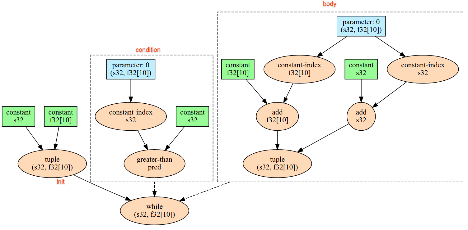
Lit un seul élément de données à partir de l'interface de flux Infeed implicite de l'appareil, en interprétant les données comme la forme donnée et sa mise en page, puis renvoie un XlaOp des données. Plusieurs opérations Infeed sont autorisées dans un calcul, mais il doit y avoir un ordre total parmi les opérations Infeed. Par exemple, deux flux Infeed dans le code ci-dessous ont un ordre total, car il existe une dépendance entre les boucles "while".
result1 = while (condition, init = init_value) {
  Infeed(shape)
}

result2 = while (condition, init = result1) {
  Infeed(shape)
}
Les formes tuples imbriquées ne sont pas acceptées. Pour une forme de tuple vide, l'opération Infeed est en fait une no-op et se poursuit sans lire les données du flux d'entrée de l'appareil.
Iota
Consultez également XlaBuilder::Iota.
Iota(shape, iota_dimension)
Crée un littéral constant sur l'appareil plutôt qu'un transfert d'hôte potentiellement volumineux. Crée un tableau avec une forme spécifiée et contient les valeurs commençant à zéro et incrémentées d'une unité le long de la dimension spécifiée. Pour les types à virgule flottante, le tableau produit est équivalent à ConvertElementType(Iota(...)), où Iota est de type intégral et que la conversion est de type à virgule flottante.
| Arguments | Type | Sémantique |
|---|---|---|
shape |
Shape |
Forme du tableau créé par Iota() |
iota_dimension |
int64 |
Dimension à incrémenter. |
Par exemple, Iota(s32[4, 8], 0) renvoie
  [[0, 0, 0, 0, 0, 0, 0, 0 ],
   [1, 1, 1, 1, 1, 1, 1, 1 ],
   [2, 2, 2, 2, 2, 2, 2, 2 ],
   [3, 3, 3, 3, 3, 3, 3, 3 ]]
Retours pour Iota(s32[4, 8], 1)
  [[0, 1, 2, 3, 4, 5, 6, 7 ],
   [0, 1, 2, 3, 4, 5, 6, 7 ],
   [0, 1, 2, 3, 4, 5, 6, 7 ],
   [0, 1, 2, 3, 4, 5, 6, 7 ]]
Map
Consultez également XlaBuilder::Map.
Map(operands..., computation)
| Arguments | Type | Sémantique |
|---|---|---|
operands |
séquence de N XlaOp |
N tableaux de types T0..T{N-1} |
computation |
XlaComputation |
un calcul de type T_0, T_1, .., T_{N + M -1} -> S avec N paramètres de type T et M de type arbitraire |
dimensions |
Tableau int64 |
tableau de dimensions de carte |
Applique une fonction scalaire sur les tableaux operands donnés, produisant ainsi un tableau aux mêmes dimensions, où chaque élément est le résultat de la fonction mappée appliquée aux éléments correspondants dans les tableaux d'entrée.
La fonction mappée est un calcul arbitraire avec la restriction selon laquelle elle comporte N entrées de type scalaire T et une seule sortie de type S. La sortie a les mêmes dimensions que les opérandes, si ce n'est que le type d'élément T est remplacé par S.
Par exemple, Map(op1, op2, op3, computation, par1) mappe elem_out <-
computation(elem1, elem2, elem3, par1) à chaque index (multidimensionnel) des tableaux d'entrée pour produire le tableau de sortie.
OptimizationBarrier
Empêche toute passe d'optimisation en déplaçant les calculs au-delà de la barrière.
Il garantit que toutes les entrées sont évaluées avant tout opérateur qui dépend des sorties de la barrière.
Coussinet
Consultez également XlaBuilder::Pad.
Pad(operand, padding_value, padding_config)
| Arguments | Type | Sémantique |
|---|---|---|
operand |
XlaOp |
tableau de type T |
padding_value |
XlaOp |
valeur scalaire de type T pour remplir la marge intérieure ajoutée |
padding_config |
PaddingConfig |
quantité de marge intérieure sur les deux bords (bas, haut) et entre les éléments de chaque dimension |
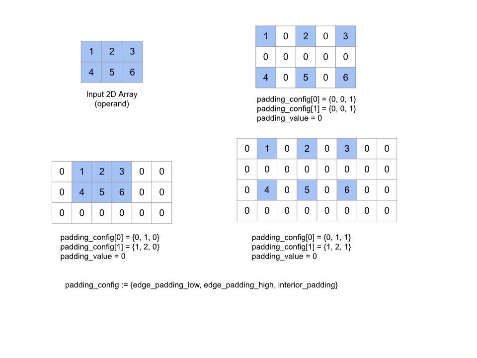
Développe le tableau operand donné en ajoutant une marge intérieure autour du tableau, ainsi qu'entre les éléments du tableau avec l'élément padding_value donné. padding_config spécifie la quantité de marge intérieure des bords et la marge intérieure intérieure pour chaque dimension.
PaddingConfig est un champ répété de PaddingConfigDimension, qui contient trois champs pour chaque dimension: edge_padding_low, edge_padding_high et interior_padding.
edge_padding_low et edge_padding_high spécifient la quantité de marge intérieure ajoutée dans la limite inférieure (à côté de l'index 0) et dans la limite supérieure (à côté de l'indice le plus élevé) de chaque dimension. La marge intérieure du bord peut être négative. La valeur absolue de la marge intérieure négative indique le nombre d'éléments à supprimer de la dimension spécifiée.
interior_padding spécifie la quantité de marge intérieure ajoutée entre deux éléments de chaque dimension. Elle ne peut pas être négative. La marge intérieure intérieure se produit de manière logique avant la marge intérieure du bord. Par conséquent, dans le cas d'une marge intérieure négative, les éléments sont supprimés de l'opérande de remplissage intérieur.
Il s'agit d'une opération no-op si les paires de marge intérieure de bordure sont toutes (0, 0) et que les valeurs de marge intérieure intérieure sont toutes égales à 0. La figure ci-dessous montre des exemples de différentes valeurs edge_padding et interior_padding pour un tableau à deux dimensions.
Recv
Consultez également XlaBuilder::Recv.
Recv(shape, channel_handle)
| Arguments | Type | Sémantique |
|---|---|---|
shape |
Shape |
forme des données à recevoir |
channel_handle |
ChannelHandle |
un identifiant unique pour chaque paire envoi/réception |
Reçoit les données de la forme donnée d'une instruction Send dans un autre calcul partageant le même identifiant de canal. Renvoie un XlaOp pour les données reçues.
L'API cliente de l'opération Recv représente une communication synchrone.
Cependant, l'instruction est décomposée en interne en deux instructions HLO (Recv et RecvDone) pour permettre les transferts de données asynchrones. Consultez également HloInstruction::CreateRecv et HloInstruction::CreateRecvDone.
Recv(const Shape& shape, int64 channel_id)
Alloue les ressources requises pour recevoir les données d'une instruction Send avec le même channel_id. Renvoie un contexte pour les ressources allouées, qui est utilisé par une instruction RecvDone suivante pour attendre la fin du transfert de données. Le contexte est un tuple de {tampon de réception (forme), identifiant de requête (U32)} et ne peut être utilisé que par une instruction RecvDone.
RecvDone(HloInstruction context)
Selon un contexte créé par une instruction Recv, attend la fin du transfert de données et renvoie les données reçues.
Réduire
Consultez également XlaBuilder::Reduce.
Applique une fonction de réduction à un ou plusieurs tableaux en parallèle.
Reduce(operands..., init_values..., computation, dimensions)
| Arguments | Type | Sémantique |
|---|---|---|
operands |
Séquence de N XlaOp |
N tableaux de types T_0, ..., T_{N-1}. |
init_values |
Séquence de N XlaOp |
N scalaires de types T_0, ..., T_{N-1}. |
computation |
XlaComputation |
un calcul de type T_0, ..., T_{N-1}, T_0, ..., T_{N-1} -> Collate(T_0, ..., T_{N-1}). |
dimensions |
Tableau int64 |
de dimensions à réduire. |
Où :
- N doit être supérieur ou égal à 1.
- Le calcul doit être "approximativement" associatif (voir ci-dessous).
- Tous les tableaux d'entrée doivent avoir les mêmes dimensions.
- Toutes les valeurs initiales doivent former une identité sous
computation. - Si la valeur est
N = 1,Collate(T)estT. - Si la valeur est
N > 1,Collate(T_0, ..., T_{N-1})est un tuple d'élémentsNde typeT.
Cette opération réduit une ou plusieurs dimensions de chaque tableau d'entrée en valeurs scalaires.
Le rang de chaque tableau renvoyé est rank(operand) - len(dimensions). Le résultat de l'opération est Collate(Q_0, ..., Q_N), où Q_i est un tableau de type T_i, dont les dimensions sont décrites ci-dessous.
Différents backends sont autorisés à réassocier le calcul de réduction. Cela peut entraîner des différences numériques, car certaines fonctions de réduction telles que l'addition ne sont pas associatives pour les floats. Toutefois, si la plage des données est limitée, l'addition à virgule flottante est suffisamment associative pour la plupart des utilisations pratiques.
Exemples
Lors de la réduction d'une dimension dans un seul tableau unidimensionnel avec des valeurs [10, 11,
12, 13], avec la fonction de réduction f (computation), le calcul est le suivant :
f(10, f(11, f(12, f(init_value, 13)))
mais il existe bien d'autres possibilités. Par exemple,
f(init_value, f(f(10, f(init_value, 11)), f(f(init_value, 12), f(init_value, 13))))
Voici un exemple de pseudo-code approximatif illustrant la mise en œuvre de la réduction, en utilisant la somme comme calcul de la réduction avec une valeur initiale de 0.
result_shape <- remove all dims in dimensions from operand_shape

# Iterate over all elements in result_shape. The number of r's here is equal
# to the rank of the result
for r0 in range(result_shape[0]), r1 in range(result_shape[1]), ...:
  # Initialize this result element
  result[r0, r1...] <- 0

  # Iterate over all the reduction dimensions
  for d0 in range(dimensions[0]), d1 in range(dimensions[1]), ...:
    # Increment the result element with the value of the operand's element.
    # The index of the operand's element is constructed from all ri's and di's
    # in the right order (by construction ri's and di's together index over the
    # whole operand shape).
    result[r0, r1...] += operand[ri... di]
Voici un exemple de réduction d'un tableau (matrice) 2D. La forme a le rang 2, la dimension 0 de taille 2 et la dimension 1 de taille 3:
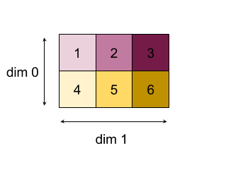
Conséquences de la réduction de 0 ou 1 des dimensions à l'aide d'une fonction "add" :
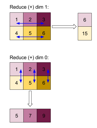
Notez que les deux résultats de réduction sont des tableaux unidimensionnels. Pour plus de commodité, l'une apparaît dans une colonne et l'autre sous forme de ligne.
Voici un exemple plus complexe : voici un tableau 3D. Son rang est 3, dimension 0 de taille 4, dimension 1 de taille 2 et dimension 2 de taille 3. Par souci de simplicité, les valeurs de 1 à 6 sont répliquées sur la dimension 0.
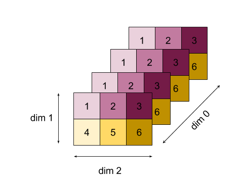
Comme dans l'exemple en 2D, nous pouvons réduire une seule dimension. Si nous réduisons la dimension 0, par exemple, nous obtenons un tableau de rang 2 dans lequel toutes les valeurs de la dimension 0 ont été pliées dans un scalaire:
|  4   8  12 |
| 16  20  24 |
Si nous réduisons la dimension 2, nous obtenons également un tableau de rang 2 dans lequel toutes les valeurs de la dimension 2 ont été pliées dans un scalaire:
| 6  15 |
| 6  15 |
| 6  15 |
| 6  15 |
Notez que l'ordre relatif entre les dimensions restantes dans l'entrée est conservé dans la sortie, mais certaines dimensions peuvent se voir attribuer de nouveaux nombres (puisque le rang change).
Nous pouvons également réduire plusieurs dimensions. La réduction des dimensions 0 et 1 génère le tableau 1D [20, 28, 36].
La réduction du tableau 3D dans toutes ses dimensions génère la valeur scalaire de 84.
Réduction variadique
Lorsque la valeur est N > 1, l'application de la fonction de réduction est légèrement plus complexe, car elle est appliquée simultanément à toutes les entrées. Les opérandes sont fournis au calcul dans l'ordre suivant:
- Exécuter la valeur réduite pour le premier opérande
- ...
- Exécuter la valeur réduite pour le n-ième opérande
- Valeur d'entrée pour le premier opérande
- ...
- Valeur d'entrée pour le n-ième opérande
Prenons l'exemple de la fonction de réduction suivante, qui permet de calculer les valeurs maximales et argmax d'un tableau unidimensionnel en parallèle:
f: (Float, Int, Float, Int) -> Float, Int
f(max, argmax, value, index):
  if value >= max:
    return (value, index)
  else:
    return (max, argmax)
Pour les tableaux d'entrée unidimensionnels V = Float[N], K = Int[N] et les valeurs d'initialisation I_V = Float, I_K = Int, le résultat f_(N-1) de la réduction dans la seule dimension d'entrée est équivalent à l'application récursive suivante:
f_0 = f(I_V, I_K, V_0, K_0)
f_1 = f(f_0.first, f_0.second, V_1, K_1)
...
f_(N-1) = f(f_(N-2).first, f_(N-2).second, V_(N-1), K_(N-1))
L'application de cette réduction à un tableau de valeurs et à un tableau d'indices séquentiels (iota) co-itéra les tableaux et renverra un tuple contenant la valeur maximale et l'index correspondant.
ReducePrecision
Consultez également XlaBuilder::ReducePrecision.
Modélise l'effet de la conversion des valeurs à virgule flottante dans un format de précision inférieure (par exemple, IEEE-FP16) et à son format d'origine. Le nombre de bits d'exposant et de mantisse au format de précision inférieure peut être spécifié de manière arbitraire, bien que toutes les tailles de bits puissent ne pas être compatibles avec toutes les implémentations matérielles.
ReducePrecision(operand, mantissa_bits, exponent_bits)
| Arguments | Type | Sémantique |
|---|---|---|
operand |
XlaOp |
tableau de type à virgule flottante T. |
exponent_bits |
int32 |
nombre de bits d'exposant dans un format de précision inférieure |
mantissa_bits |
int32 |
nombre de bits de mantisse dans un format de précision inférieure |
Le résultat est un tableau de type T. Les valeurs d'entrée sont arrondies à la valeur la plus proche représentable par le nombre donné de bits de mantisse (à l'aide de la sémantique "jointe à pair"), et toutes les valeurs qui dépassent la plage spécifiée par le nombre de bits d'exposant sont limitées à l'infini positif ou négatif. Les valeurs NaN sont conservées, bien qu'elles puissent être converties en valeurs NaN canoniques.
Le format de précision inférieure doit avoir au moins un bit d'exposant (afin de distinguer une valeur nulle d'une infinité, car tous deux ont une mantisse nulle) et doit comporter un nombre non négatif de bits de mantisse. Le nombre de bits d'exposant ou de mantisse peut dépasser la valeur correspondante pour le type T. La partie correspondante de la conversion est alors simplement une no-op.
ReduceScatter
Consultez également XlaBuilder::ReduceScatter.
Réduit la dispersion est une opération collective qui effectue de manière efficace une réduction d'impact, puis disperse le résultat en le divisant en blocs shard_count le long de l'élément scatter_dimension, et l'instance répliquée i dans le groupe d'instances répliquées reçoit le fragment ith.
ReduceScatter(operand, computation, scatter_dim, shard_count,
replica_group_ids, channel_id)
| Arguments | Type | Sémantique |
|---|---|---|
operand |
XlaOp |
Tableau ou tuple de tableaux non vide à réduire sur le nombre d'instances répliquées. |
computation |
XlaComputation |
Calcul de la réduction |
scatter_dimension |
int64 |
Dimension à disperser. |
shard_count |
int64 |
Nombre de blocs à diviser scatter_dimension |
replica_groups |
vecteur de vecteurs de int64 |
Groupes entre lesquels les réductions sont effectuées |
channel_id |
(Facultatif) int64 |
ID de canal facultatif pour la communication entre les modules |
- Lorsque
operandest un tuple de tableaux, la réduction de la dispersion est effectuée sur chaque élément du tuple. replica_groupsest une liste de groupes d'instances répliquées entre lesquels la réduction est effectuée (l'ID de l'instance répliquée de l'instance répliquée actuelle peut être récupéré à l'aide deReplicaId). L'ordre des instances répliquées dans chaque groupe détermine l'ordre dans lequel le résultat de la réduction complète sera dispersé.replica_groupsdoit être vide (auquel cas toutes les instances répliquées appartiennent à un seul groupe) ou contenir le même nombre d'éléments que le nombre d'instances répliquées. Lorsqu'il y a plusieurs groupes d'instances répliquées, ils doivent tous avoir la même taille. Par exemple,replica_groups = {0, 2}, {1, 3}effectue une réduction entre les instances répliquées0et2, ainsi que1et3, puis disperse le résultat.shard_countest la taille de chaque groupe d'instances répliquées. Nous en avons besoin dans les cas oùreplica_groupsest vide. Sireplica_groupsn'est pas vide,shard_countdoit être égal à la taille de chaque groupe d'instances répliquées.channel_idest utilisé pour la communication entre les modules: seules les opérationsreduce-scatterayant le mêmechannel_idpeuvent communiquer entre elles.
La forme de sortie correspond à la forme d'entrée avec la scatter_dimension réduite de shard_count fois. Par exemple, s'il existe deux instances répliquées et que l'opérande possède respectivement les valeurs [1.0, 2.25] et [3.0, 5.25] sur les deux instances répliquées, la valeur de sortie de cette opération où scatter_dim est 0 sera [4.0] pour la première instance répliquée et [7.5] pour la deuxième.
ReduceWindow
Consultez également XlaBuilder::ReduceWindow.
Applique une fonction de réduction à tous les éléments de chaque fenêtre d'une séquence de N tableaux multidimensionnels, produisant ainsi un seul ou un tuple de N tableaux multidimensionnels en sortie. Chaque tableau de sortie contient le même nombre d'éléments que le nombre de positions valides de la fenêtre. Une couche de pooling peut être exprimée sous la forme d'un ReduceWindow. Comme pour Reduce, le computation appliqué reçoit toujours le init_values à gauche.
ReduceWindow(operands..., init_values..., computation, window_dimensions,
window_strides, padding)
| Arguments | Type | Sémantique |
|---|---|---|
operands |
N XlaOps |
Séquence de N tableaux multidimensionnels de types T_0,..., T_{N-1}, chacun représentant la zone de base sur laquelle la fenêtre est placée. |
init_values |
N XlaOps |
N valeurs de départ de la réduction, une pour chacun des N opérandes. Pour en savoir plus, consultez Réduire. |
computation |
XlaComputation |
Fonction de réduction de type T_0, ..., T_{N-1}, T_0, ..., T_{N-1} -> Collate(T_0, ..., T_{N-1}), à appliquer aux éléments de chaque fenêtre de tous les opérandes d'entrée. |
window_dimensions |
ArraySlice<int64> |
tableau d'entiers pour les valeurs de dimension de fenêtre |
window_strides |
ArraySlice<int64> |
tableau d'entiers pour les valeurs de pas de fenêtre |
base_dilations |
ArraySlice<int64> |
tableau d'entiers pour les valeurs de dilation de base |
window_dilations |
ArraySlice<int64> |
tableau d'entiers pour les valeurs de dilatation de la fenêtre |
padding |
Padding |
Type de marge intérieure pour la fenêtre (Padding::kSame, qui crée la même forme de sortie pour avoir la même forme de sortie que l'entrée si le pas a la valeur 1, ou Padding::kValid, qui n'utilise pas de marge intérieure et "arrête" la fenêtre lorsqu'elle ne rentre plus) |
Où :
- N doit être supérieur ou égal à 1.
- Tous les tableaux d'entrée doivent avoir les mêmes dimensions.
- Si la valeur est
N = 1,Collate(T)estT. - Si la valeur est
N > 1,Collate(T_0, ..., T_{N-1})est un tuple d'élémentsNde type(T0,...T{N-1}).
La figure et le code ci-dessous illustrent un exemple d'utilisation de ReduceWindow. L'entrée est une
matrice de taille [4x6], et window_dimensions et window_stride_dimensions correspondent à [2x3].
// Create a computation for the reduction (maximum).
XlaComputation max;
{
  XlaBuilder builder(client_, "max");
  auto y = builder.Parameter(0, ShapeUtil::MakeShape(F32, {}), "y");
  auto x = builder.Parameter(1, ShapeUtil::MakeShape(F32, {}), "x");
  builder.Max(y, x);
  max = builder.Build().value();
}

// Create a ReduceWindow computation with the max reduction computation.
XlaBuilder builder(client_, "reduce_window_2x3");
auto shape = ShapeUtil::MakeShape(F32, {4, 6});
auto input = builder.Parameter(0, shape, "input");
builder.ReduceWindow(
    input,
    /*init_val=*/builder.ConstantLiteral(LiteralUtil::MinValue(F32)),
    *max,
    /*window_dimensions=*/{2, 3},
    /*window_stride_dimensions=*/{2, 3},
    Padding::kValid);
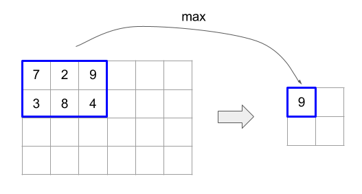
Un pas de 1 dans une dimension indique que la position d'une fenêtre dans la dimension est à 1 élément de sa fenêtre adjacente. Pour qu'aucune fenêtre ne se chevauche, window_stride_dimensions doit être égal à window_dimensions. La figure ci-dessous illustre l'utilisation de deux valeurs de pas différentes. La marge intérieure est appliquée à chaque dimension de l'entrée, et les calculs sont les mêmes que si l'entrée venait avec les dimensions qu'elle a après la marge intérieure.
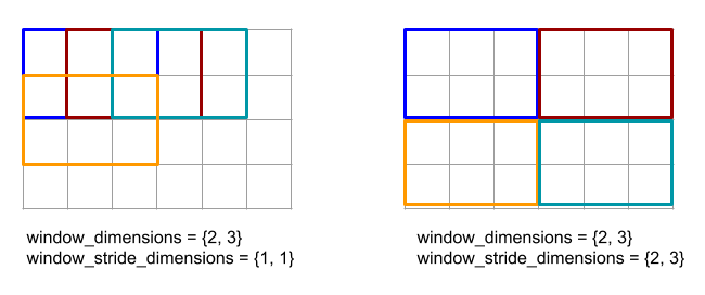
Pour un exemple de marge intérieure non négligeable, envisagez de calculer la valeur minimale de réduction de la fenêtre (la valeur initiale est MAX_FLOAT) avec la dimension 3 et de placer 2 sur le tableau d'entrée [10000, 1000, 100, 10, 1]. La marge intérieure kValid calcule les valeurs minimales sur deux fenêtres valides: [10000, 1000, 100] et [100, 10, 1], ce qui génère la sortie [100, 1]. La marge intérieure kSame remplit d'abord le tableau de sorte que la forme après la fenêtre de réduction soit identique à l'entrée pour le pas 1 en ajoutant les éléments initiaux des deux côtés, ce qui donne [MAX_VALUE, 10000, 1000, 100, 10, 1,
MAX_VALUE]. L'exécution de la fonction "réduction de la fenêtre" sur le tableau rempli fonctionne sur trois fenêtres [MAX_VALUE, 10000, 1000], [1000, 100, 10] et [10, 1, MAX_VALUE], et avec un rendement [1000, 10, 1].
L'ordre d'évaluation de la fonction de réduction est arbitraire et peut être non déterministe. Par conséquent, la fonction de réduction ne doit pas être trop sensible à la réassociation. Pour en savoir plus, consultez la discussion sur l'associativité dans le contexte de Reduce.
ReplicaId
Consultez également XlaBuilder::ReplicaId.
Renvoie l'identifiant unique (scalaire U32) de l'instance répliquée.
ReplicaId()
L'ID unique de chaque instance répliquée est un entier non signé situé dans l'intervalle [0, N), où N correspond au nombre d'instances répliquées. Étant donné que toutes les instances répliquées exécutent le même programme, un appel ReplicaId() dans le programme renvoie une valeur différente sur chaque instance répliquée.
Remodeler
Consultez également XlaBuilder::Reshape et l'opération Collapse.
Remanie les dimensions d'un tableau dans une nouvelle configuration.
Reshape(operand, new_sizes)
Reshape(operand, dimensions, new_sizes)
| Arguments | Type | Sémantique |
|---|---|---|
operand |
XlaOp |
tableau de type T |
dimensions |
Vecteur int64 |
l'ordre dans lequel les dimensions sont réduites |
new_sizes |
Vecteur int64 |
vecteur de tailles de nouvelles dimensions |
D'un point de vue conceptuel, cette méthode consiste d'abord à aplatir un tableau en un vecteur unidimensionnel de valeurs de données, puis à affiner ce vecteur dans une nouvelle forme. Les arguments d'entrée sont un tableau arbitraire de type T, un vecteur de constante de temps de compilation d'indices de dimension et un vecteur de constante de temps de compilation de tailles de dimension pour le résultat.
Les valeurs du vecteur dimension, si elles sont fournies, doivent être une permutation de toutes les dimensions de T. Si elles ne sont pas fournies, la valeur par défaut est {0, ..., rank - 1}. L'ordre des dimensions dans dimensions va de la dimension la plus lente (la plus majeure) à la dimension la plus rapide (la plus mineure) dans l'imbrication de boucle, ce qui réduit le tableau d'entrée en une seule dimension. Le vecteur new_sizes détermine la taille du tableau de sortie. La valeur à l'indice 0 dans new_sizes correspond à la taille de la dimension 0, la valeur à l'indice 1 est à la taille de la dimension 1, et ainsi de suite. Le produit des dimensions new_size doit être égal au produit des tailles des dimensions de l'opérande. Lorsque vous affinez le tableau réduit pour obtenir le tableau multidimensionnel défini par new_sizes, les dimensions de new_sizes sont classées de la variation la plus lente (la plus importante) à la plus la plus rapide (la plus mineure).
Par exemple, supposons que "v" soit un tableau de 24 éléments:
let v = f32[4x2x3] { { {10, 11, 12}, {15, 16, 17} },
                    { {20, 21, 22}, {25, 26, 27} },
                    { {30, 31, 32}, {35, 36, 37} },
                    { {40, 41, 42}, {45, 46, 47} } };

In-order collapse:
let v012_24 = Reshape(v, {0,1,2}, {24});
then v012_24 == f32[24] {10, 11, 12, 15, 16, 17, 20, 21, 22, 25, 26, 27,
                         30, 31, 32, 35, 36, 37, 40, 41, 42, 45, 46, 47};

let v012_83 = Reshape(v, {0,1,2}, {8,3});
then v012_83 == f32[8x3] { {10, 11, 12}, {15, 16, 17},
                          {20, 21, 22}, {25, 26, 27},
                          {30, 31, 32}, {35, 36, 37},
                          {40, 41, 42}, {45, 46, 47} };

Out-of-order collapse:
let v021_24 = Reshape(v, {1,2,0}, {24});
then v012_24 == f32[24]  {10, 20, 30, 40, 11, 21, 31, 41, 12, 22, 32, 42,
                          15, 25, 35, 45, 16, 26, 36, 46, 17, 27, 37, 47};

let v021_83 = Reshape(v, {1,2,0}, {8,3});
then v021_83 == f32[8x3] { {10, 20, 30}, {40, 11, 21},
                          {31, 41, 12}, {22, 32, 42},
                          {15, 25, 35}, {45, 16, 26},
                          {36, 46, 17}, {27, 37, 47} };


let v021_262 = Reshape(v, {1,2,0}, {2,6,2});
then v021_262 == f32[2x6x2] { { {10, 20}, {30, 40},
                              {11, 21}, {31, 41},
                              {12, 22}, {32, 42} },
                             { {15, 25}, {35, 45},
                              {16, 26}, {36, 46},
                              {17, 27}, {37, 47} } };
Dans un cas particulier, la modification de forme peut transformer un tableau à un seul élément en scalaire, et inversement. Par exemple,
Reshape(f32[1x1] { {5} }, {0,1}, {}) == 5;
Reshape(5, {}, {1,1}) == f32[1x1] { {5} };
Retour (inverse)
Consultez également XlaBuilder::Rev.
Rev(operand, dimensions)
| Arguments | Type | Sémantique |
|---|---|---|
operand |
XlaOp |
tableau de type T |
dimensions |
ArraySlice<int64> |
de dimensions à inverser |
Inverse l'ordre des éléments du tableau operand selon la dimensions spécifiée, générant un tableau de sortie de même forme. Chaque élément du tableau d'opérandes à un indice multidimensionnel est stocké dans le tableau de sortie à un indice transformé. L'indice multidimensionnel est transformé en inversant
l'index dans chaque dimension à inverser (autrement dit, si une dimension de taille N est l'une des dimensions inverses, son index i est transformé en N - 1 - i).
L'opération Rev permet, entre autres, d'inverser le tableau de pondérations de convolution selon les dimensions des deux fenêtres lors du calcul du gradient dans les réseaux de neurones.
RngNormal
Consultez également XlaBuilder::RngNormal.
Construit une sortie d'une forme donnée avec des nombres aléatoires générés suivant la \(N(\mu, \sigma)\) distribution normale. Les paramètres \(\mu\) et \(\sigma\), ainsi que la forme de sortie, doivent être de type élémentaire à virgule flottante. De plus, les paramètres doivent avoir une valeur scalaire.
RngNormal(mu, sigma, shape)
| Arguments | Type | Sémantique |
|---|---|---|
mu |
XlaOp |
Scalaire de type T spécifiant la moyenne des nombres générés |
sigma |
XlaOp |
Scalaire de type T spécifiant l'écart type de la valeur générée |
shape |
Shape |
Forme de sortie de type T |
RngUniform
Consultez également XlaBuilder::RngUniform.
Construit la sortie d'une forme donnée avec des nombres aléatoires générés après la distribution uniforme sur l'intervalle \([a,b)\). Les paramètres et le type d'élément de sortie doivent être de type booléen, intégral ou à virgule flottante, et les types doivent être cohérents. Les backends de processeur et de GPU ne sont actuellement compatibles qu'avec F64, F32, F16, BF16, S64, U64, S32 et U32. De plus, les paramètres doivent avoir une valeur scalaire. Si \(b <= a\) , le résultat est défini par l'implémentation.
RngUniform(a, b, shape)
| Arguments | Type | Sémantique |
|---|---|---|
a |
XlaOp |
Scalaire de type T spécifiant la limite inférieure de l'intervalle |
b |
XlaOp |
Scalaire de type T spécifiant la limite supérieure de l'intervalle |
shape |
Shape |
Forme de sortie de type T |
RngBitGenerator
Génère une sortie avec une forme donnée remplie de bits aléatoires uniformes à l'aide de l'algorithme spécifié (ou par défaut du backend), puis renvoie un état mis à jour (avec la même forme que l'état initial) ainsi que les données aléatoires générées.
L'état initial est l'état initial de la génération actuelle de nombres aléatoires. Cette valeur, ainsi que la forme et les valeurs valides requises, dépendent de l'algorithme utilisé.
La sortie sera forcément une fonction déterministe de l'état initial, mais il n'est pas garanti qu'elle soit déterministe entre les backends et les différentes versions du compilateur.
RngBitGenerator(algorithm, key, shape)
| Arguments | Type | Sémantique |
|---|---|---|
algorithm |
RandomAlgorithm |
Algorithme de PRNG à utiliser. |
initial_state |
XlaOp |
État initial de l'algorithme de PRNG. |
shape |
Shape |
Forme de sortie pour les données générées. |
Valeurs disponibles pour algorithm:
rng_default: algorithme spécifique au backend avec des exigences de forme spécifiques au backend.rng_three_fry: algorithme de PRNG basé sur un compteur ThreeFry La formeinitial_stateestu64[2]avec des valeurs arbitraires. Salmon et al. SC, 2011. Avec des nombres aléatoires parallèles, c'est très simple: 1, 2, 3.rng_philox: algorithme Philox permettant de générer des nombres aléatoires en parallèle La formeinitial_stateestu64[3]avec des valeurs arbitraires. Salmon et al. SC, 2011. Avec des nombres aléatoires parallèles, c'est très simple: 1, 2, 3.
Nuage de points
L'opération de dispersion XLA génère une séquence de résultats correspondant aux valeurs du tableau d'entrée operands, avec plusieurs tranches (aux index spécifiés par scatter_indices) mises à jour avec la séquence de valeurs dans updates à l'aide de update_computation.
Consultez également XlaBuilder::Scatter.
scatter(operands..., scatter_indices, updates..., update_computation,
index_vector_dim, update_window_dims, inserted_window_dims,
scatter_dims_to_operand_dims)
| Arguments | Type | Sémantique |
|---|---|---|
operands |
Séquence de N XlaOp |
N tableaux de types T_0, ..., T_N dans lesquels la dispersion est appliquée. |
scatter_indices |
XlaOp |
Tableau contenant les indices de départ des tranches sur lesquelles la distribution doit s'appliquer. |
updates |
Séquence de N XlaOp |
N tableaux de types T_0, ..., T_N. updates[i] contient les valeurs à utiliser pour diffuser operands[i]. |
update_computation |
XlaComputation |
Calcul à utiliser pour combiner les valeurs existantes dans le tableau d'entrée et les mises à jour lors de la diffusion. Ce calcul doit être de type T_0, ..., T_N, T_0, ..., T_N -> Collate(T_0, ..., T_N). |
index_vector_dim |
int64 |
Dimension dans scatter_indices contenant les index de départ. |
update_window_dims |
ArraySlice<int64> |
Ensemble des dimensions de la forme updates qui sont des dimensions de fenêtre. |
inserted_window_dims |
ArraySlice<int64> |
Ensemble des dimensions de la fenêtre qui doit être insérée dans la forme updates. |
scatter_dims_to_operand_dims |
ArraySlice<int64> |
Carte de dimensions entre les indices de dispersion et l'espace d'indice de l'opérande. Ce tableau est interprété comme mappant i à scatter_dims_to_operand_dims[i] . Elle doit être de type un à un et total. |
indices_are_sorted |
bool |
Indique si le tri des index est garanti par l'appelant. |
Où :
- N doit être supérieur ou égal à 1.
operands[0], ...,operands[N-1] doit tous avoir les mêmes dimensions.updates[0], ...,updates[N-1] doit tous avoir les mêmes dimensions.- Si la valeur est
N = 1,Collate(T)estT. - Si la valeur est
N > 1,Collate(T_0, ..., T_N)est un tuple d'élémentsNde typeT.
Si index_vector_dim est égal à scatter_indices.rank, nous considérons implicitement que scatter_indices a une dimension 1 à la fin.
Nous définissons update_scatter_dims de type ArraySlice<int64> comme l'ensemble des dimensions de la forme updates qui ne sont pas dans update_window_dims, dans l'ordre croissant.
Les arguments de dispersion doivent respecter les contraintes suivantes:
Chaque tableau
updatesdoit être de rangupdate_window_dims.size + scatter_indices.rank - 1.Les limites de la dimension
idans chaque tableauupdatesdoivent respecter ce qui suit:- Si
iest présent dansupdate_window_dims(c'est-à-dire égal àupdate_window_dims[k] pour certainsk), la limite de la dimensionidansupdatesne doit pas dépasser la limite correspondante deoperandaprès avoir pris en compteinserted_window_dims(par exemple,adjusted_window_bounds[k], oùadjusted_window_boundscontient les limites deoperandavec les limites des indexinserted_window_dimssupprimées). - Si
iest présent dansupdate_scatter_dims(c'est-à-dire,update_scatter_dims[k] pour certainsk), la limite de la dimensionidansupdatesdoit être égale à la limite correspondante descatter_indices, en ignorantindex_vector_dim(par exemple,scatter_indices.shape.dims[k], sik<index_vector_dimetscatter_indices.shape.dims[k+1] dans le cas contraire).
- Si
update_window_dimsdoit être dans l'ordre croissant, ne pas avoir de numéros de dimension répétés et être compris dans la plage[0, updates.rank).inserted_window_dimsdoit être dans l'ordre croissant, ne pas avoir de numéros de dimension répétés et être compris dans la plage[0, operand.rank).operand.rankdoit être égal à la somme deupdate_window_dims.sizeetinserted_window_dims.size.scatter_dims_to_operand_dims.sizedoit être égal àscatter_indices.shape.dims[index_vector_dim], et ses valeurs doivent être comprises dans la plage[0, operand.rank).
Pour un indice U donné dans chaque tableau updates, l'index I correspondant dans le tableau operands correspondant auquel cette mise à jour doit être appliquée est calculé comme suit:
- Soit
G= {U[k] pourkdansupdate_scatter_dims}. UtilisezGpour rechercher un vecteur d'indiceSdans le tableauscatter_indices, de sorte queS[i] =scatter_indices[Combine(G,i)] où Combine(A, b) insère b aux positionsindex_vector_dimdans A. - Créez un index
Sindansoperandà l'aide deSen dispersantSà l'aide de la mapscatter_dims_to_operand_dims. Plus formellement :Sin[scatter_dims_to_operand_dims[k]] =S[k] sik<scatter_dims_to_operand_dims.size.Sin[_] =0dans les autres cas.
- Créez un indice
Windans chaque tableauoperandsen dispersant les indices au niveau deupdate_window_dimsdansUen fonction deinserted_window_dims. Plus formellement :Win[window_dims_to_operand_dims(k)] =U[k] sikse trouve dansupdate_window_dims, oùwindow_dims_to_operand_dimsest la fonction monotone avec le domaine [0,update_window_dims.size) et la plage [0,operand.rank) \inserted_window_dims. (Par exemple, siupdate_window_dims.sizeest4,operand.rankest6etinserted_window_dimsest {0,2},window_dims_to_operand_dimsest {0→1,1→3,2→4,3→5}.)Win[_] =0dans les autres cas.
Icorrespond àWin+Sin, où + correspond à l'addition au niveau de l'élément.
En résumé, l'opération de dispersion peut être définie comme suit.
- Initialisez
outputavecoperands, c'est-à-dire pour tous les indexJ, pour tous les indicesOdans le tableauoperands[J] :
output[J][O] =operands[J][O] - Pour chaque indice
Udu tableauupdates[J] et l'index correspondantOdans le tableauoperand[J], siOest un indice valide pouroutput:
(output[0][O], ...,output[N-1][O]) =update_computation(output[0][O], ..., ,output[N-1][O],updates[0][U], ...,updates[N-1][U])
L'ordre dans lequel les mises à jour sont appliquées est non déterministe. Ainsi, lorsque plusieurs indices dans updates font référence au même index dans operands, la valeur correspondante dans output est non déterministe.
Notez que le premier paramètre transmis dans update_computation sera toujours la valeur actuelle du tableau output et que le deuxième paramètre correspondra toujours à la valeur du tableau updates. Ceci est particulièrement important dans les cas où update_computation n'est pas commutatif.
Si indices_are_sorted est défini sur "true", XLA peut supposer que les start_indices sont triés (dans l'ordre croissant de start_index_map) par l'utilisateur. Si ce n'est pas le cas, la sémantique est définie.
De façon informelle, l'opération de dispersion peut être considérée comme l'inverse de l'opération de regroupement, c'est-à-dire qu'elle met à jour les éléments de l'entrée extraits par l'opération de collecte correspondante.
Pour obtenir une description informelle et détaillée, consultez la section "Description informelle" sous Gather.
Sélectionner
Consultez également XlaBuilder::Select.
Construit un tableau de sortie à partir des éléments de deux tableaux d'entrée, en fonction des valeurs d'un tableau de prédicats.
Select(pred, on_true, on_false)
| Arguments | Type | Sémantique |
|---|---|---|
pred |
XlaOp |
tableau de type PRED |
on_true |
XlaOp |
tableau de type T |
on_false |
XlaOp |
tableau de type T |
Les tableaux on_true et on_false doivent avoir la même forme. Il s'agit également de la forme du tableau de sortie. Le tableau pred doit avoir la même dimension que on_true et on_false, avec le type d'élément PRED.
Pour chaque élément P de pred, l'élément correspondant du tableau de sortie est extrait de on_true si la valeur de P est true et de on_false si la valeur de P est false. En tant que forme limitée de diffusion, pred peut être un scalaire de type PRED. Dans ce cas, le tableau de sortie est entièrement extrait de on_true si pred est true, et de on_false si pred est false.
Exemple avec un pred non scalaire:
let pred: PRED[4] = {true, false, false, true};
let v1: s32[4] = {1, 2, 3, 4};
let v2: s32[4] = {100, 200, 300, 400};
==>
Select(pred, v1, v2) = s32[4]{1, 200, 300, 4};
Exemple avec un pred scalaire:
let pred: PRED = true;
let v1: s32[4] = {1, 2, 3, 4};
let v2: s32[4] = {100, 200, 300, 400};
==>
Select(pred, v1, v2) = s32[4]{1, 2, 3, 4};
Les sélections entre tuples sont acceptées. À cette fin, les tuples sont considérés comme des types scalaires. Si on_true et on_false sont des tuples (qui doivent avoir la même forme), pred doit être un scalaire de type PRED.
SelectAndScatter
Consultez également XlaBuilder::SelectAndScatter.
Cette opération peut être considérée comme une opération composite qui calcule d'abord ReduceWindow sur le tableau operand pour sélectionner un élément dans chaque fenêtre, puis disperse le tableau source entre les index des éléments sélectionnés pour construire un tableau de sortie ayant la même forme que le tableau d'opérandes. La fonction binaire select permet de sélectionner un élément dans chaque fenêtre en l'appliquant à chaque fenêtre. Elle est appelée avec la propriété selon laquelle le vecteur d'index du premier paramètre est lexicographiquement inférieur au vecteur d'index du deuxième paramètre. La fonction select renvoie true si le premier paramètre est sélectionné et renvoie false si le deuxième est sélectionné. La fonction doit maintenir la transitivité (par exemple, si select(a, b) et select(b, c) sont true, alors select(a, c) est également true) afin que l'élément sélectionné ne dépende pas de l'ordre des éléments parcourus pour une fenêtre donnée.
La fonction scatter est appliquée à chaque index sélectionné dans le tableau de sortie. Elle nécessite deux paramètres scalaires:
- Valeur actuelle à l'index sélectionné dans le tableau de sortie
- Valeur de dispersion de
sourcequi s'applique à l'index sélectionné
Elle combine les deux paramètres et renvoie une valeur scalaire permettant de mettre à jour la valeur au niveau de l'index sélectionné dans le tableau de sortie. Initialement, tous les index du tableau de sortie sont définis sur init_value.
Le tableau de sortie a la même forme que le tableau operand, et le tableau source doit avoir la même forme qu'à la suite de l'application d'une opération ReduceWindow sur le tableau operand. SelectAndScatter permet de rétropropager les valeurs de gradient d'une couche de pooling dans un réseau de neurones.
SelectAndScatter(operand, select, window_dimensions, window_strides,
padding, source, init_value, scatter)
| Arguments | Type | Sémantique |
|---|---|---|
operand |
XlaOp |
tableau de type T sur lequel les fenêtres glissent |
select |
XlaComputation |
Calcul binaire de type T, T -> PRED à appliquer à tous les éléments de chaque fenêtre. Renvoie true si le premier paramètre est sélectionné et false si le deuxième paramètre est sélectionné. |
window_dimensions |
ArraySlice<int64> |
tableau d'entiers pour les valeurs de dimension de fenêtre |
window_strides |
ArraySlice<int64> |
tableau d'entiers pour les valeurs de pas de fenêtre |
padding |
Padding |
Type de marge intérieure pour la fenêtre (Padding::kSame ou Padding::kValid) |
source |
XlaOp |
tableau de type T avec les valeurs à disperser |
init_value |
XlaOp |
valeur scalaire de type T pour la valeur initiale du tableau de sortie |
scatter |
XlaComputation |
Calcul binaire de type T, T -> T, pour appliquer chaque élément source à nuage de points avec son élément de destination |
La figure ci-dessous montre des exemples d'utilisation de SelectAndScatter, dans laquelle la fonction select calcule la valeur maximale parmi ses paramètres. Notez que lorsque les fenêtres se chevauchent, comme dans la figure (2) ci-dessous, un index du tableau operand peut être sélectionné plusieurs fois par différentes fenêtres. Dans la figure, l'élément de valeur 9 est sélectionné par les deux fenêtres supérieures (bleu et rouge), et la fonction d'addition binaire scatter génère l'élément de sortie de valeur 8 (2 + 6).
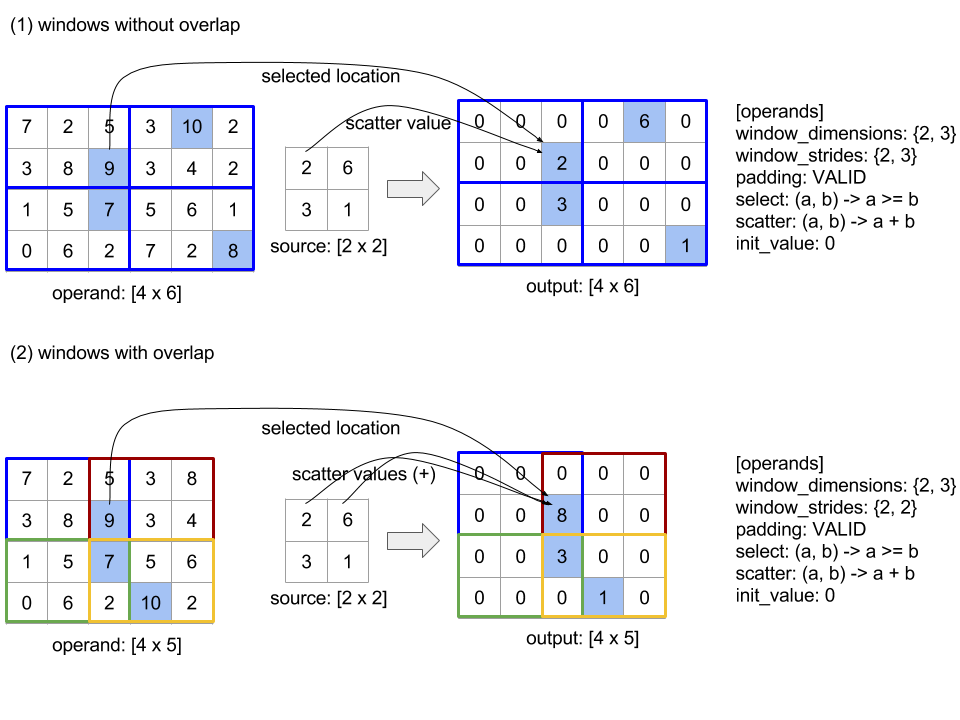
L'ordre d'évaluation de la fonction scatter est arbitraire et peut être non déterministe. Par conséquent, la fonction scatter ne doit pas être trop sensible à la réassociation. Pour en savoir plus, consultez la discussion sur l'associativité dans le contexte de Reduce.
Envoyer
Consultez également XlaBuilder::Send.
Send(operand, channel_handle)
| Arguments | Type | Sémantique |
|---|---|---|
operand |
XlaOp |
données à envoyer (tableau de type T) |
channel_handle |
ChannelHandle |
un identifiant unique pour chaque paire envoi/réception |
Envoie les données d'opérande fournies à une instruction Recv dans un autre calcul qui partage le même identifiant de canal. Ne renvoie aucune donnée.
Comme pour l'opération Recv, l'API cliente de l'opération Send représente une communication synchrone. Elle est décomposée en interne en deux instructions HLO (Send et SendDone) pour permettre les transferts de données asynchrones. Consultez également HloInstruction::CreateSend et HloInstruction::CreateSendDone.
Send(HloInstruction operand, int64 channel_id)
Lance un transfert asynchrone de l'opérande vers les ressources allouées par l'instruction Recv avec le même ID de canal. Renvoie un contexte qui est utilisé par une instruction SendDone suivante pour attendre la fin du transfert de données. Le contexte est un tuple de {opérande (forme), identifiant de requête (U32)} et ne peut être utilisé que par une instruction SendDone.
SendDone(HloInstruction context)
Compte tenu d'un contexte créé par une instruction Send, attend la fin du transfert de données. L'instruction ne renvoie aucune donnée.
Programmation des instructions pour la chaîne
L'ordre d'exécution des quatre instructions pour chaque canal (Recv, RecvDone, Send, SendDone) est le suivant.
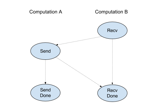
Recva lieu avant leSendSenda lieu avant leRecvDoneRecva lieu avant leRecvDoneSenda lieu avant leSendDone
Lorsque les compilateurs de backend génèrent une programmation linéaire pour chaque calcul qui communique via des instructions de canal, il ne doit pas y avoir de cycles entre les calculs. Par exemple, les programmations ci-dessous entraînent des interblocages.
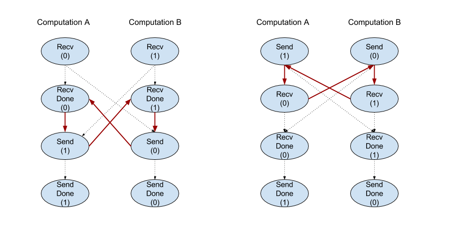
Tranche
Consultez également XlaBuilder::Slice.
Le découpage extrait un sous-tableau du tableau d'entrée. Le sous-tableau a le même rang que l'entrée et contient les valeurs à l'intérieur d'un cadre de délimitation au sein du tableau d'entrée, où les dimensions et les index du cadre de délimitation sont fournis en tant qu'arguments pour l'opération de tranche.
Slice(operand, start_indices, limit_indices, strides)
| Arguments | Type | Sémantique |
|---|---|---|
operand |
XlaOp |
Tableau à N dimensions de type T |
start_indices |
ArraySlice<int64> |
Liste des N entiers contenant les index de départ de la tranche pour chaque dimension. Les valeurs doivent être supérieures ou égales à zéro. |
limit_indices |
ArraySlice<int64> |
Liste des N entiers contenant les index de fin (exclus) de la tranche pour chaque dimension. Chaque valeur doit être supérieure ou égale à la valeur start_indices correspondant à la dimension et inférieure ou égale à la taille de la dimension. |
strides |
ArraySlice<int64> |
Liste de N entiers qui détermine le pas d'entrée de la tranche. Le segment sélectionne tous les éléments strides[d] de la dimension d. |
Exemple unidimensionnel:
let a = {0.0, 1.0, 2.0, 3.0, 4.0}
Slice(a, {2}, {4}) produces:
  {2.0, 3.0}
Exemple en deux dimensions:
let b =
 { {0.0,  1.0,  2.0},
   {3.0,  4.0,  5.0},
   {6.0,  7.0,  8.0},
   {9.0, 10.0, 11.0} }

Slice(b, {2, 1}, {4, 3}) produces:
  { { 7.0,  8.0},
    {10.0, 11.0} }
Trier
Consultez également XlaBuilder::Sort.
Sort(operands, comparator, dimension, is_stable)
| Arguments | Type | Sémantique |
|---|---|---|
operands |
ArraySlice<XlaOp> |
Opérandes à trier. |
comparator |
XlaComputation |
Le calcul de comparaison à utiliser. |
dimension |
int64 |
Dimension selon laquelle le tri est effectué. |
is_stable |
bool |
Indique si le tri stable doit être utilisé. |
Si un seul opérande est fourni:
Si l'opérande est un Tensor de rang 1 (un tableau), le résultat est un tableau trié. Si vous souhaitez trier le tableau dans l'ordre croissant, le comparateur doit effectuer une comparaison "inférieur à". Officiellement, une fois le tableau trié, il contient pour toutes les positions d'index
i, javeci < jquecomparator(value[i], value[j]) = comparator(value[j], value[i]) = falseoucomparator(value[i], value[j]) = true.Si l'opérande a un rang plus élevé, il est trié en fonction de la dimension fournie. Par exemple, pour un Tensor de rang 2 (une matrice), une valeur de dimension de
0trie indépendamment chaque colonne, et une valeur de dimension1trie indépendamment chaque ligne. Si aucun numéro de dimension n'est fourni, la dernière dimension est choisie par défaut. Pour la dimension triée, le même ordre de tri s'applique que dans le cas de rang-1.
Si des opérandes n > 1 sont fournis:
Tous les opérandes
ndoivent être des Tensors de mêmes dimensions. Les types d'éléments des Tensors peuvent être différents.Tous les opérandes sont triés ensemble, et non individuellement. Conceptuellement, les opérandes sont traités comme un tuple. Lorsque vous vérifiez si les éléments de chaque opérande aux positions d'index
ietjdoivent être échangés, le comparateur est appelé avec les paramètres scalaires2 * n, où le paramètre2 * kcorrespond à la valeur à la positionide l'opérandek-thet le paramètre2 * k + 1à la valeur à la positionjde l'opérandek-th. En règle générale, le comparateur compare les paramètres2 * ket2 * k + 1entre eux et peut utiliser d'autres paires de paramètres comme points de rupture.Le résultat est un tuple qui se compose des opérandes dans l'ordre trié (le long de la dimension fournie, comme ci-dessus). L'opérande
i-thdu tuple correspond à l'opérandei-thde Sort.
Par exemple, s'il existe trois opérandes operand0 = [3, 1], operand1 = [42, 50] et operand2 = [-3.0, 1.1], et que le comparateur ne compare que les valeurs de operand0 avec "inférieur à", la sortie du tri est le tuple ([1, 3], [50, 42], [1.1, -3.0]).
Si is_stable est défini sur "true", le tri est stable. En d'autres termes, si des éléments sont considérés comme égaux par le comparateur, l'ordre relatif des valeurs égales est conservé. Deux éléments e1 et e2 sont égaux si et seulement si comparator(e1, e2) = comparator(e2, e1) = false. Par défaut, is_stable est défini sur "false".
Transpose
Consultez également l'opération tf.reshape.
Transpose(operand)
| Arguments | Type | Sémantique |
|---|---|---|
operand |
XlaOp |
Opérande à transposer. |
permutation |
ArraySlice<int64> |
Comment réactiver les dimensions |
Permute les dimensions de l'opérande avec la permutation donnée, donc ∀ i . 0 ≤ i < rank ⇒ input_dimensions[permutation[i]] = output_dimensions[i].
C'est la même chose que Reshape(opérande, permutation, Permute(permutation, opérande.shape.dimensions)).
TriangularSolve
Consultez également XlaBuilder::TriangularSolve.
Résoudre des systèmes d'équations linéaires comportant des matrices de coefficients triangulaires inférieurs ou supérieurs par substitution ou contre-substitution. En utilisant des dimensions principales, cette routine résout l'un des systèmes matriciels op(a) * x =
b, ou x * op(a) = b, pour la variable x, en fonction de a et b, où op(a) est op(a) = a, op(a) = Transpose(a) ou op(a) = Conj(Transpose(a)).
TriangularSolve(a, b, left_side, lower, unit_diagonal, transpose_a)
| Arguments | Type | Sémantique |
|---|---|---|
a |
XlaOp |
un rang > 2 tableau de type complexe ou à virgule flottante avec la forme [..., M, M]. |
b |
XlaOp |
un tableau de rang > 2 du même type avec la forme [..., M, K] si left_side est "true", [..., K, M] dans le cas contraire. |
left_side |
bool |
indique s'il faut résoudre un système de la forme op(a) * x = b (true) ou x * op(a) = b (false). |
lower |
bool |
choisir d'utiliser le triangle supérieur ou inférieur de a. |
unit_diagonal |
bool |
Si la valeur est true, les éléments diagonaux de a sont considérés comme 1 et ne sont pas accessibles. |
transpose_a |
Transpose |
choisir d'utiliser a tel quel, de le transposer ou d'utiliser sa transposition conjuguée. |
Les données d'entrée sont lues uniquement à partir du triangle inférieur/supérieur de a, en fonction de la valeur de lower. Les valeurs de l'autre triangle sont ignorées. Les données de sortie sont renvoyées dans le même triangle. Les valeurs de l'autre triangle sont définies par l'implémentation et peuvent être n'importe quoi.
Si le rang de a et b est supérieur à 2, ils sont traités comme des lots de matrices, où toutes, à l'exception des deux dimensions mineures, sont des dimensions de lot. a et b doivent avoir les mêmes dimensions de lot.
Tuple
Consultez également XlaBuilder::Tuple.
tuple contenant un nombre variable de poignées de données, chacun ayant sa propre forme.
C'est semblable à std::tuple en C++. D'un point de vue conceptuel:
let v: f32[10] = f32[10]{0, 1, 2, 3, 4, 5, 6, 7, 8, 9};
let s: s32 = 5;
let t: (f32[10], s32) = tuple(v, s);
Les tuples peuvent être décomposés (accessibles) via l'opération GetTupleElement.
Bien que
Consultez également XlaBuilder::While.
While(condition, body, init)
| Arguments | Type | Sémantique |
|---|---|---|
condition |
XlaComputation |
XlaComputation de type T -> PRED qui définit la condition d'arrêt de la boucle. |
body |
XlaComputation |
XlaComputation de type T -> T qui définit le corps de la boucle. |
init |
T |
Valeur initiale pour le paramètre condition et body. |
Exécute body de manière séquentielle jusqu'à l'échec de condition. Cette méthode est semblable à une boucle "while" classique dans de nombreux autres langages, à l'exception des différences et des restrictions indiquées ci-dessous.
- Un nœud
Whilerenvoie une valeur de typeT, qui est le résultat de la dernière exécution debody. - La forme du type
Test déterminée de manière statique et doit être identique dans toutes les itérations.
Les paramètres T des calculs sont initialisés avec la valeur init lors de la première itération et sont automatiquement mis à jour vers le nouveau résultat de body à chaque itération suivante.
L'un des principaux cas d'utilisation du nœud While consiste à implémenter l'exécution répétée de l'entraînement dans les réseaux de neurones. Le pseudo-code simplifié est illustré ci-dessous avec un graphique qui représente le calcul. Vous trouverez ce code dans while_test.cc.
Le type T dans cet exemple est un Tuple composé d'un int32 pour le nombre d'itérations et d'un vector[10] pour l'accumulateur. Pendant 1 000 itérations, la boucle continue d'ajouter un vecteur constant à l'accumulateur.
// Pseudocode for the computation.
init = {0, zero_vector[10]} // Tuple of int32 and float[10].
result = init;
while (result(0) < 1000) {
  iteration = result(0) + 1;
  new_vector = result(1) + constant_vector[10];
  result = {iteration, new_vector};
}