در زیر معنای عملیات تعریف شده در رابط XlaBuilder را شرح می دهد. به طور معمول، این عملیات یک به یک به عملیات تعریف شده در رابط RPC در xla_data.proto نگاشت.
نکته ای در مورد نامگذاری: نوع داده تعمیم یافته ای که XLA با آن سروکار دارد، یک آرایه N بعدی است که عناصری از نوع یکنواخت (مانند شناور ۳۲ بیتی) را در خود نگه می دارد. در سراسر مستندات، آرایه برای نشان دادن یک آرایه با ابعاد دلخواه استفاده می شود. برای راحتی، موارد خاص نام های خاص و آشناتری دارند. به عنوان مثال یک بردار یک آرایه 1 بعدی و یک ماتریس یک آرایه دو بعدی است.
گذشته از همه اینها
XlaBuilder::AfterAll نیز ببینید.
AfterAll تعداد متغیری توکن را می گیرد و یک توکن تولید می کند. توکنها انواع اولیهای هستند که میتوان آنها را بین عملیاتهای جانبی قرار داد تا سفارش را اجرا کنند. AfterAll می توان به عنوان پیوندی از نشانه ها برای سفارش عملیات پس از یک مجموعه عملیات استفاده کرد.
AfterAll(operands)
| استدلال ها | تایپ کنید | مفاهیم |
|---|---|---|
operands | XlaOp | تعداد متغیر توکن ها |
همه جمع شوند
XlaBuilder::AllGather نیز ببینید.
الحاق بین کپی ها را انجام می دهد.
AllGather(operand, all_gather_dim, shard_count, replica_group_ids, channel_id)
| استدلال ها | تایپ کنید | مفاهیم |
|---|---|---|
operand | XlaOp | آرایه ای برای الحاق بین کپی ها |
all_gather_dim | int64 | بعد الحاق |
replica_groups | بردار بردارهای int64 | گروه هایی که الحاق بین آنها انجام می شود |
channel_id | اختیاری int64 | شناسه کانال اختیاری برای ارتباط متقابل ماژول |
-
replica_groupsلیستی از گروههای replica است که الحاق بین آنها انجام میشود (شناسه replica برای ماکت فعلی را میتوان با استفاده ازReplicaIdبازیابی کرد). ترتیب تکرارها در هر گروه تعیین کننده ترتیب قرار گرفتن ورودی های آنها در نتیجه است.replica_groupsیا باید خالی باشند (در این صورت همه کپیها متعلق به یک گروه واحد هستند که از0تاN - 1مرتب شدهاند)، یا دارای همان تعداد عناصر با تعداد کپیها باشند. برای مثال،replica_groups = {0, 2}, {1, 3}الحاق بین replica های0و2و1و3را انجام می دهد. -
shard_countاندازه هر گروه ماکت است. در مواردی کهreplica_groupsخالی هستند به این نیاز داریم. -
channel_idبرای ارتباط متقابل ماژول استفاده می شود: فقط عملیاتall-gatherبا همانchannel_idمی توانند با یکدیگر ارتباط برقرار کنند.
شکل خروجی شکل ورودی با all_gather_dim است که shard_count بار بزرگتر شده است. به عنوان مثال، اگر دو replica وجود داشته باشد و عملوند دارای مقدار [1.0, 2.5] و [3.0, 5.25] به ترتیب روی دو replica باشد، آنگاه مقدار خروجی از این عملیات که در آن all_gather_dim 0 است [1.0, 2.5, 3.0, 5.25] خواهد بود. [1.0, 2.5, 3.0, 5.25] در هر دو ماکت.
همه کاهش
XlaBuilder::AllReduce نیز ببینید.
یک محاسبات سفارشی در بین کپی ها انجام می دهد.
AllReduce(operand, computation, replica_group_ids, channel_id)
| استدلال ها | تایپ کنید | مفاهیم |
|---|---|---|
operand | XlaOp | آرایه یا چند تایی از آرایههای خالی برای کاهش بین ماکتها |
computation | XlaComputation | محاسبه کاهش |
replica_groups | بردار بردارهای int64 | گروه هایی که بین آنها کاهش ها انجام می شود |
channel_id | اختیاری int64 | شناسه کانال اختیاری برای ارتباط متقابل ماژول |
- هنگامی که
operandچند آرایه است، کاهش همه روی هر عنصر تاپل انجام می شود. -
replica_groupsفهرستی از گروههای replica است که بین آنها کاهش انجام میشود (شناسه replica برای replica فعلی را میتوان با استفاده ازReplicaIdبازیابی کرد).replica_groupsیا باید خالی باشد (در این صورت همه replica ها متعلق به یک گروه واحد هستند)، یا دارای همان تعداد عناصر با تعداد Replica ها باشند. برای مثال،replica_groups = {0, 2}, {1, 3}بین کپیهای0و2و1و3کاهش میدهد. -
channel_idبرای ارتباطات متقابل ماژول استفاده میشود: فقط عملیاتهایall-reduceبا همانchannel_idمیتوانند با یکدیگر ارتباط برقرار کنند.
شکل خروجی همان شکل ورودی است. به عنوان مثال، اگر دو replica وجود داشته باشد و عملوند دارای مقدار [1.0, 2.5] و [3.0, 5.25] به ترتیب روی دو replica باشد، آنگاه مقدار خروجی از این عملیات و محاسبه جمع در هر دو [4.0, 7.75] خواهد بود. ماکت ها اگر ورودی یک تاپلی باشد، خروجی نیز یک تاپل است.
محاسبه نتیجه AllReduce مستلزم داشتن یک ورودی از هر ماکت است، بنابراین اگر یک ماکت یک گره AllReduce را بیشتر از دیگری اجرا کند، آنگاه ماکت قبلی برای همیشه منتظر خواهد ماند. از آنجایی که کپیها همه یک برنامه را اجرا میکنند، راههای زیادی برای این کار وجود ندارد، اما زمانی ممکن است که شرایط حلقه while به دادههای ورودی بستگی داشته باشد و دادههایی که وارد میشوند باعث شوند حلقه while بارها تکرار شود. روی یک ماکت نسبت به دیگری
AllToAll
XlaBuilder::AllToAll نیز ببینید.
AllToAll یک عملیات جمعی است که داده ها را از همه هسته ها به همه هسته ها ارسال می کند. دو فاز دارد:
- فاز پراکندگی. در هر هسته، عملوند به تعداد بلوکهای
split_countدر امتدادsplit_dimensionsتقسیم میشود، و بلوکها به همه هستهها پراکنده میشوند، به عنوان مثال، بلوک ith به هسته i ارسال میشود. - مرحله جمع آوری هر هسته بلوک های دریافتی را در امتداد
concat_dimensionبه هم متصل می کند.
هسته های شرکت کننده را می توان توسط:
-
replica_groups: هر ReplicaGroup حاوی لیستی از Replica IDهای شرکت کننده در محاسبه است (شناسه replica برای replica فعلی را می توان با استفاده ازReplicaIdبازیابی کرد). AllToAll در زیر گروه ها به ترتیب مشخص شده اعمال خواهد شد. برای مثال،replica_groups = { {1,2,3}, {4,5,0} }به این معنی است که یک AllToAll در کپیهای{1, 2, 3}و در مرحله جمعآوری اعمال میشود و بلوکهای دریافتی به همان ترتیب 1، 2، 3 الحاق شود. سپس، AllToAll دیگری در کپی های 4، 5، 0 اعمال می شود، و ترتیب الحاق نیز 4، 5، 0 است. اگرreplica_groupsخالی باشد، همه کپی ها متعلق به یک هستند. گروه، به ترتیب الحاق ظاهرشان.
پیش نیازها:
- اندازه بعد عملوند در
split_dimensionبرsplit_countقابل تقسیم است. - شکل عملوند تاپلی نیست.
AllToAll(operand, split_dimension, concat_dimension, split_count, replica_groups)
| استدلال ها | تایپ کنید | مفاهیم |
|---|---|---|
operand | XlaOp | n آرایه ورودی بعدی |
split_dimension | int64 | مقداری در بازه [0, n) که ابعادی را که عملوند در امتداد آن تقسیم میشود نامگذاری میکند |
concat_dimension | int64 | مقداری در بازه [0, n) که ابعادی را که بلوک های تقسیم شده در امتداد آن به هم پیوسته اند نام می برد. |
split_count | int64 | تعداد هسته هایی که در این عملیات شرکت می کنند. اگر replica_groups خالی است، این باید تعداد replica ها باشد. در غیر این صورت، این باید برابر با تعداد کپی در هر گروه باشد. |
replica_groups | وکتور ReplicaGroup | هر گروه حاوی لیستی از شناسه های ماکت است. |
در زیر نمونه ای از Alltoall را نشان می دهد.
XlaBuilder b("alltoall");
auto x = Parameter(&b, 0, ShapeUtil::MakeShape(F32, {4, 16}), "x");
AllToAll(x, /*split_dimension=*/1, /*concat_dimension=*/0, /*split_count=*/4);
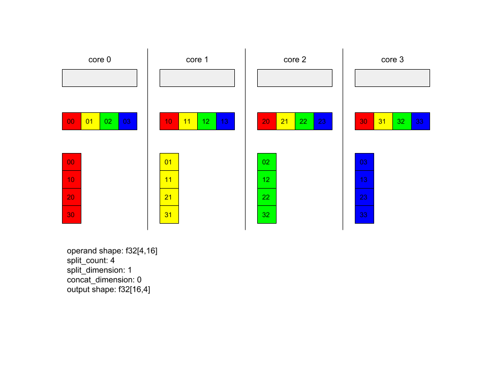
در این مثال، 4 هسته در Alltoall شرکت دارند. در هر هسته، عملوند در امتداد بعد 0 به 4 قسمت تقسیم می شود، بنابراین هر قسمت دارای شکل f32 [4،4] است. 4 قسمت در تمام هسته ها پراکنده شده اند. سپس هر هسته قطعات دریافتی را در امتداد ابعاد 1 به ترتیب هسته 0-4 به هم متصل می کند. بنابراین خروجی هر هسته دارای شکل f32 [16,4] است.
BatchNormGrad
همچنین XlaBuilder::BatchNormGrad و مقاله نرمال سازی دسته اصلی را برای توضیح دقیق الگوریتم ببینید.
گرادیان های هنجار دسته ای را محاسبه می کند.
BatchNormGrad(operand, scale, mean, variance, grad_output, epsilon, feature_index)
| استدلال ها | تایپ کنید | مفاهیم |
|---|---|---|
operand | XlaOp | n آرایه بعدی باید نرمال شود (x) |
scale | XlaOp | آرایه 1 بعدی (\(\gamma\)) |
mean | XlaOp | آرایه 1 بعدی (\(\mu\)) |
variance | XlaOp | آرایه 1 بعدی (\(\sigma^2\)) |
grad_output | XlaOp | گرادیان ها به BatchNormTraining (\(\nabla y\)) منتقل شد |
epsilon | float | مقدار اپسیلون (\(\epsilon\)) |
feature_index | int64 | شاخص به بعد ویژگی در operand |
برای هر ویژگی در بعد ویژگی ( feature_index شاخص بعد ویژگی در operand است)، این عملیات گرادیان ها را با توجه به operand ، offset و scale در تمام ابعاد دیگر محاسبه می کند. feature_index باید یک شاخص معتبر برای بعد ویژگی در operand باشد.
سه گرادیان با فرمول های زیر تعریف می شوند (با فرض یک آرایه 4 بعدی به عنوان operand و با شاخص بعد ویژگی l ، اندازه دسته ای m و اندازه های فضایی w و h ):
\[ \begin{split} c_l&= \frac{1}{mwh}\sum_{i=1}^m\sum_{j=1}^w\sum_{k=1}^h \left( \nabla y_{ijkl} \frac{x_{ijkl} - \mu_l}{\sigma^2_l+\epsilon} \right) \\\\ d_l&= \frac{1}{mwh}\sum_{i=1}^m\sum_{j=1}^w\sum_{k=1}^h \nabla y_{ijkl} \\\\ \nabla x_{ijkl} &= \frac{\gamma_{l} }{\sqrt{\sigma^2_{l}+\epsilon} } \left( \nabla y_{ijkl} - d_l - c_l (x_{ijkl} - \mu_{l}) \right) \\\\ \nabla \gamma_l &= \sum_{i=1}^m\sum_{j=1}^w\sum_{k=1}^h \left( \nabla y_{ijkl} \frac{x_{ijkl} - \mu_l}{\sqrt{\sigma^2_{l}+\epsilon} } \right) \\\\\ \nabla \beta_l &= \sum_{i=1}^m\sum_{j=1}^w\sum_{k=1}^h \nabla y_{ijkl} \end{split} \]
mean و variance ورودی ها مقادیر گشتاورها را در ابعاد دسته ای و فضایی نشان می دهد.
نوع خروجی سه دسته است:
| خروجی ها | تایپ کنید | مفاهیم |
|---|---|---|
grad_operand | XlaOp | گرادیان با توجه به operand ورودی ($\nabla x$) |
grad_scale | XlaOp | گرادیان با توجه به scale ورودی ($\nabla \gamma$) |
grad_offset | XlaOp | گرادیان با توجه به offset ورودی ($\nabla \beta$) |
BatchNormInference
همچنین XlaBuilder::BatchNormInference و مقاله نرمال سازی دسته اصلی را برای توضیح دقیق الگوریتم ببینید.
یک آرایه را در ابعاد دسته ای و فضایی عادی می کند.
BatchNormInference(operand, scale, offset, mean, variance, epsilon, feature_index)
| استدلال ها | تایپ کنید | مفاهیم |
|---|---|---|
operand | XlaOp | n آرایه بعدی عادی شود |
scale | XlaOp | آرایه 1 بعدی |
offset | XlaOp | آرایه 1 بعدی |
mean | XlaOp | آرایه 1 بعدی |
variance | XlaOp | آرایه 1 بعدی |
epsilon | float | ارزش اپسیلون |
feature_index | int64 | شاخص به بعد ویژگی در operand |
برای هر ویژگی در بعد ویژگی ( feature_index شاخص بعد ویژگی در operand است)، این عملیات میانگین و واریانس را در تمام ابعاد دیگر محاسبه می کند و از میانگین و واریانس برای عادی سازی هر عنصر در operand استفاده می کند. feature_index باید یک شاخص معتبر برای بعد ویژگی در operand باشد.
BatchNormInference معادل فراخوانی BatchNormTraining بدون محاسبه mean و variance برای هر دسته است. در عوض از mean ورودی و variance به عنوان مقادیر تخمینی استفاده می کند. هدف از این عملیات کاهش تأخیر در استنتاج است، از این رو BatchNormInference نامیده می شود.
خروجی یک آرایه n بعدی و نرمال شده با همان شکل operand ورودی است.
BatchNormTraining
همچنین XlaBuilder::BatchNormTraining و the original batch normalization paper برای توضیح دقیق الگوریتم ببینید.
یک آرایه را در ابعاد دسته ای و فضایی عادی می کند.
BatchNormTraining(operand, scale, offset, epsilon, feature_index)
| استدلال ها | تایپ کنید | مفاهیم |
|---|---|---|
operand | XlaOp | n آرایه بعدی باید نرمال شود (x) |
scale | XlaOp | آرایه 1 بعدی (\(\gamma\)) |
offset | XlaOp | آرایه 1 بعدی (\(\beta\)) |
epsilon | float | مقدار اپسیلون (\(\epsilon\)) |
feature_index | int64 | شاخص به بعد ویژگی در operand |
برای هر ویژگی در بعد ویژگی ( feature_index شاخص بعد ویژگی در operand است)، این عملیات میانگین و واریانس را در تمام ابعاد دیگر محاسبه می کند و از میانگین و واریانس برای عادی سازی هر عنصر در operand استفاده می کند. feature_index باید یک شاخص معتبر برای بعد ویژگی در operand باشد.
الگوریتم برای هر دسته در operand \(x\) که شامل m عناصر با w و h به اندازه ابعاد فضایی است (با فرض اینکه operand یک آرایه 4 بعدی است) به شرح زیر است:
میانگین دسته ای \(\mu_l\) را برای هر ویژگی
lدر بعد ویژگی محاسبه می کند:\(\mu_l=\frac{1}{mwh}\sum_{i=1}^m\sum_{j=1}^w\sum_{k=1}^h x_{ijkl}\)واریانس دسته ای \(\sigma^2_l\)را محاسبه می کند: $\sigma^2 l=\frac{1}{mwh}\sum {i=1}^m\sum {j=1}^w\sum {k=1}^h ( x_{ijkl} - \mu_l)^2$
عادی، مقیاس و جابجایی:\(y_{ijkl}=\frac{\gamma_l(x_{ijkl}-\mu_l)}{\sqrt[2]{\sigma^2_l+\epsilon} }+\beta_l\)
مقدار اپسیلون، معمولاً یک عدد کوچک، برای جلوگیری از خطاهای تقسیم بر صفر اضافه می شود.
نوع خروجی سه تایی XlaOp است:
| خروجی ها | تایپ کنید | مفاهیم |
|---|---|---|
output | XlaOp | n آرایه بعدی با همان شکل operand ورودی (y) |
batch_mean | XlaOp | آرایه 1 بعدی (\(\mu\)) |
batch_var | XlaOp | آرایه 1 بعدی (\(\sigma^2\)) |
batch_mean و batch_var گشتاورهایی هستند که در ابعاد دسته ای و فضایی با استفاده از فرمول های بالا محاسبه می شوند.
BitcastConvertType
XlaBuilder::BitcastConvertType را نیز ببینید.
مشابه یک tf.bitcast در TensorFlow، عملیات بیتکست عنصری را از شکل داده به شکل هدف انجام می دهد. اندازه ورودی و خروجی باید مطابقت داشته باشند: به عنوان مثال، عناصر s32 از طریق روال بیتکست به عناصر f32 تبدیل میشوند و یک عنصر s32 به چهار عنصر s8 تبدیل میشود. بیتکست بهعنوان یک بازیگر سطح پایین پیادهسازی میشود، بنابراین ماشینهایی با نمایشهای ممیز شناور متفاوت نتایج متفاوتی خواهند داشت.
BitcastConvertType(operand, new_element_type)
| استدلال ها | تایپ کنید | مفاهیم |
|---|---|---|
operand | XlaOp | آرایه از نوع T با کم نور D |
new_element_type | PrimitiveType | نوع U |
ابعاد عملوند و شکل هدف باید مطابقت داشته باشند، جدای از آخرین بعد که با نسبت اندازه اولیه قبل و بعد از تبدیل تغییر می کند.
نوع عنصر مبدا و مقصد نباید چند تایی باشد.
تبدیل بیتکست به نوع اولیه با عرض های مختلف
دستور BitcastConvert HLO از حالتی پشتیبانی می کند که اندازه عنصر خروجی نوع T' با اندازه عنصر ورودی T برابر نباشد. از آنجایی که کل عملیات از نظر مفهومی یک بیتکست است و بایتهای زیرین را تغییر نمیدهد، شکل عنصر خروجی باید تغییر کند. برای B = sizeof(T), B' = sizeof(T') ، دو حالت ممکن وجود دارد.
ابتدا، وقتی B > B' ، شکل خروجی یک بعد جزئی جدید به اندازه B/B' می گیرد. مثلا:
f16[10,2]{1,0} %output = f16[10,2]{1,0} bitcast-convert(f32[10]{0} %input)
این قانون برای اسکالرهای موثر یکسان است:
f16[2]{0} %output = f16[2]{0} bitcast-convert(f32[] %input)
روش دیگر، برای B' > B ، دستورالعمل نیاز دارد که آخرین بعد منطقی شکل ورودی برابر با B'/B باشد، و این بعد در طول تبدیل حذف میشود:
f32[10]{0} %output = f32[10]{0} bitcast-convert(f16[10,2]{1,0} %input)
توجه داشته باشید که تبدیل بین پهنای بیت های مختلف عنصری نیست.
پخش
XlaBuilder::Broadcast نیز ببینید.
با کپی کردن داده ها در آرایه، ابعاد را به آرایه اضافه می کند.
Broadcast(operand, broadcast_sizes)
| استدلال ها | تایپ کنید | مفاهیم |
|---|---|---|
operand | XlaOp | آرایه برای کپی کردن |
broadcast_sizes | ArraySlice<int64> | اندازه های ابعاد جدید |
ابعاد جدید در سمت چپ درج می شوند، یعنی اگر broadcast_sizes دارای مقادیر {a0, ..., aN} و شکل عملوند دارای ابعاد {b0, ..., bM} باشد، شکل خروجی دارای ابعاد {a0, ..., aN, b0, ..., bM} .
ابعاد جدید به کپی هایی از عملوند ایندکس می شود، به عنوان مثال
output[i0, ..., iN, j0, ..., jM] = operand[j0, ..., jM]
به عنوان مثال، اگر operand اسکالر f32 با مقدار 2.0f باشد، و broadcast_sizes {2, 3} باشد، نتیجه آرایه ای با شکل f32[2, 3] خواهد بود و تمام مقادیر در نتیجه 2.0f خواهد بود.
BroadcastInDim
XlaBuilder::BroadcastInDim نیز ببینید.
اندازه و رتبه یک آرایه را با کپی کردن داده ها در آرایه گسترش می دهد.
BroadcastInDim(operand, out_dim_size, broadcast_dimensions)
| استدلال ها | تایپ کنید | مفاهیم |
|---|---|---|
operand | XlaOp | آرایه برای کپی کردن |
out_dim_size | ArraySlice<int64> | اندازه ابعاد شکل هدف |
broadcast_dimensions | ArraySlice<int64> | هر بعد از شکل عملوند مربوط به کدام بعد در شکل هدف است |
مشابه Broadcast، اما امکان افزودن ابعاد در هر نقطه و گسترش ابعاد موجود با اندازه 1 را می دهد.
operand به شکل توصیف شده توسط out_dim_size پخش می شود. broadcast_dimensions ابعاد operand را به ابعاد شکل هدف نگاشت میکند، یعنی بعد i'م عملوند به بعد broadcast_dimension[i]'مین شکل خروجی نگاشت میشود. ابعاد operand باید اندازه 1 داشته باشد یا به اندازه ابعاد در شکل خروجی که به آن نگاشت شده اند باشد. ابعاد باقیمانده با ابعاد اندازه 1 پر می شود. پخش با ابعاد منحط سپس در امتداد این ابعاد منحط پخش می شود تا به شکل خروجی برسد. معناشناسی به طور مفصل در صفحه پخش توضیح داده شده است.
زنگ زدن
XlaBuilder::Call نیز ببینید.
محاسبه ای را با آرگومان های داده شده فراخوانی می کند.
Call(computation, args...)
| استدلال ها | تایپ کنید | مفاهیم |
|---|---|---|
computation | XlaComputation | محاسبات نوع T_0, T_1, ..., T_{N-1} -> S با N پارامتر از نوع دلخواه |
args | دنباله ای از N XlaOp s | N آرگومان از نوع دلخواه |
آریتی و انواع args باید با پارامترهای computation مطابقت داشته باشد. بدون args مجاز است.
چولسکی
XlaBuilder::Cholesky نیز ببینید.
تجزیه Cholesky دسته ای از ماتریس های قطعی مثبت متقارن (Hermitian) را محاسبه می کند.
Cholesky(a, lower)
| استدلال ها | تایپ کنید | مفاهیم |
|---|---|---|
a | XlaOp | یک آرایه رتبه > 2 از نوع پیچیده یا ممیز شناور. |
lower | bool | از مثلث بالایی یا پایینی a استفاده کنیم. |
اگر lower true باشد، ماتریس های مثلثی پایین l به گونه ای محاسبه می کند که $a = l باشد. l^T$. اگر lower false باشد، ماتریسهای مثلثی بالا u بهگونهای محاسبه میکند که\(a = u^T . u\).
بسته به مقدار lower ، داده های ورودی فقط از مثلث پایین/بالایی a خوانده می شود. مقادیر از مثلث دیگر نادیده گرفته می شوند. داده های خروجی در همان مثلث برگردانده می شوند. مقادیر در مثلث دیگر با پیاده سازی تعریف شده اند و ممکن است هر چیزی باشند.
اگر رتبه a بزرگتر از 2 باشد، a به عنوان دسته ای از ماتریس ها در نظر گرفته می شود، که در آن همه ابعاد به جز 2 جزئی، ابعاد دسته ای هستند.
اگر a متقارن (Hermitian) مثبت قطعی نباشد، نتیجه اجرا تعریف می شود.
گیره
XlaBuilder::Clamp نیز ببینید.
یک عملوند را در محدوده بین یک مقدار حداقل و حداکثر قرار می دهد.
Clamp(min, operand, max)
| استدلال ها | تایپ کنید | مفاهیم |
|---|---|---|
min | XlaOp | آرایه از نوع T |
operand | XlaOp | آرایه از نوع T |
max | XlaOp | آرایه از نوع T |
با توجه به یک عملوند و مقادیر حداقل و حداکثر، اگر در محدوده بین حداقل و حداکثر باشد، عملوند را برمیگرداند، در غیر این صورت اگر عملوند زیر این محدوده باشد، مقدار حداقل و اگر عملوند بالاتر از این محدوده باشد، مقدار حداکثر را برمیگرداند. یعنی clamp(a, x, b) = min(max(a, x), b) .
هر سه آرایه باید یک شکل باشند. از طرف دیگر، به عنوان یک شکل محدود پخش ، min و/یا max میتواند یک اسکالر از نوع T باشد.
مثال با min و max اسکالر:
let operand: s32[3] = {-1, 5, 9};
let min: s32 = 0;
let max: s32 = 6;
==>
Clamp(min, operand, max) = s32[3]{0, 5, 6};
سقوط - فروپاشی
همچنین XlaBuilder::Collapse و عملیات tf.reshape را ببینید.
ابعاد یک آرایه را در یک بعد جمع می کند.
Collapse(operand, dimensions)
| استدلال ها | تایپ کنید | مفاهیم |
|---|---|---|
operand | XlaOp | آرایه از نوع T |
dimensions | وکتور int64 | به ترتیب، زیر مجموعه های متوالی از ابعاد T. |
Collapse زیر مجموعه داده شده از ابعاد عملوند را با یک بعد منفرد جایگزین می کند. آرگومان های ورودی یک آرایه دلخواه از نوع T و یک بردار ثابت-زمان کامپایل از شاخص های بعد هستند. شاخصهای ابعاد باید یک مرتبه (اعداد ابعاد کم تا زیاد)، زیرمجموعهای متوالی از ابعاد T باشند. بنابراین، {0، 1، 2}، {0، 1}، یا {1، 2} همه مجموعههای ابعاد معتبر هستند، اما {1، 0} یا {0، 2} نیستند. آنها با یک بعد جدید جایگزین می شوند، در همان موقعیت در ترتیب ابعادی که جایگزین می شوند، با اندازه ابعاد جدید برابر با حاصلضرب اندازه های ابعاد اصلی. کمترین عدد بعد در dimensions ، کندترین بعد متغیر (بزرگترین) در لانه حلقه است که این ابعاد را جمع می کند، و بالاترین عدد بعد سریعترین تغییر (فرع ترین) است. در صورت نیاز به سفارش جمعبندی کلیتر، عملگر tf.reshape را ببینید.
به عنوان مثال، فرض کنید v آرایه ای از 24 عنصر باشد:
let v = f32[4x2x3] { { {10, 11, 12},  {15, 16, 17} },
{ {20, 21, 22},  {25, 26, 27} },
{ {30, 31, 32},  {35, 36, 37} },
{ {40, 41, 42},  {45, 46, 47} } };

// Collapse to a single dimension, leaving one dimension.
let v012 = Collapse(v, {0,1,2});
then v012 == f32[24] {10, 11, 12, 15, 16, 17,
20, 21, 22, 25, 26, 27,
30, 31, 32, 35, 36, 37,
40, 41, 42, 45, 46, 47};

// Collapse the two lower dimensions, leaving two dimensions.
let v01 = Collapse(v, {0,1});
then v01 == f32[4x6] { {10, 11, 12, 15, 16, 17},
{20, 21, 22, 25, 26, 27},
{30, 31, 32, 35, 36, 37},
{40, 41, 42, 45, 46, 47} };

// Collapse the two higher dimensions, leaving two dimensions.
let v12 = Collapse(v, {1,2});
then v12 == f32[8x3] { {10, 11, 12},
{15, 16, 17},
{20, 21, 22},
{25, 26, 27},
{30, 31, 32},
{35, 36, 37},
{40, 41, 42},
{45, 46, 47} };
CollectivePermute
XlaBuilder::CollectivePermute را نیز ببینید.
CollectivePermute یک عملیات جمعی است که داده های متقاطع را ارسال و دریافت می کند.
CollectivePermute(operand, source_target_pairs)
| استدلال ها | تایپ کنید | مفاهیم |
|---|---|---|
operand | XlaOp | n آرایه ورودی بعدی |
source_target_pairs | بردار <int64, int64> | لیستی از جفت های (source_replica_id، target_replica_id). برای هر جفت، عملوند از replica مبدا به replica هدف ارسال می شود. |
توجه داشته باشید که محدودیت های زیر برای source_target_pair وجود دارد:
- هر دو جفت نباید شناسه ماکت هدف یکسانی داشته باشند، و نباید شناسه ماکت منبع یکسانی داشته باشند.
- اگر یک Replica id در هیچ جفتی هدف نباشد، خروجی آن ماکت یک تانسور متشکل از 0(s) با همان شکل ورودی است.
الحاق
XlaBuilder::ConcatInDim را نیز ببینید.
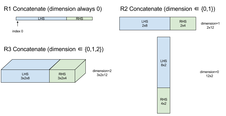
Concatenate یک آرایه از چند عملوند آرایه می سازد. آرایه با هر یک از عملوندهای آرایه ورودی (که باید هم رتبه یکدیگر باشند) رتبه یکسانی دارد و آرگومان ها را به ترتیبی که مشخص کرده اند، در خود دارد.
Concatenate(operands..., dimension)
| استدلال ها | تایپ کنید | مفاهیم |
|---|---|---|
operands | دنباله ای از N XlaOp | N آرایه از نوع T با ابعاد [L0, L1, ...]. به N >= 1 نیاز دارد. |
dimension | int64 | مقداری در بازه [0, N) که ابعادی را که باید بین operands الحاق شود نام میبرد. |
به استثنای dimension همه ابعاد باید یکسان باشند. این به این دلیل است که XLA از آرایههای "راگ" پشتیبانی نمیکند. همچنین توجه داشته باشید که مقادیر رتبه-0 را نمی توان به هم متصل کرد (زیرا نام بعدی که در آن الحاق اتفاق می افتد غیرممکن است).
مثال 1 بعدی:
Concat({ {2, 3}, {4, 5}, {6, 7} }, 0)
>>> {2, 3, 4, 5, 6, 7}
مثال دو بعدی:
let a = {
{1, 2},
{3, 4},
{5, 6},
};
let b = {
{7, 8},
};
Concat({a, b}, 0)
>>> {
{1, 2},
{3, 4},
{5, 6},
{7, 8},
}
نمودار:
مشروط
XlaBuilder::Conditional نیز ببینید.
Conditional(pred, true_operand, true_computation, false_operand, false_computation)
| استدلال ها | تایپ کنید | مفاهیم |
|---|---|---|
pred | XlaOp | اسکالر از نوع PRED |
true_operand | XlaOp | آرگومان نوع \(T_0\) |
true_computation | XlaComputation | محاسبات Xla از نوع \(T_0 \to S\) |
false_operand | XlaOp | آرگومان نوع \(T_1\) |
false_computation | XlaComputation | محاسبات Xla از نوع \(T_1 \to S\) |
اگر pred true باشد true_computation اگر pred false باشد false_computation را اجرا میکند و نتیجه را برمیگرداند.
true_computation باید در یک آرگومان واحد از نوع \(T_0\) باشد و با true_operand که باید از همان نوع باشد فراخوانی می شود. false_computation باید یک آرگومان منفرد از نوع \(T_1\) داشته باشد و با false_operand که باید از همان نوع باشد فراخوانی می شود. نوع مقدار بازگشتی true_computation و false_computation باید یکسان باشد.
توجه داشته باشید که فقط یکی از true_computation و false_computation بسته به مقدار pred اجرا خواهد شد.
Conditional(branch_index, branch_computations, branch_operands)
| استدلال ها | تایپ کنید | مفاهیم |
|---|---|---|
branch_index | XlaOp | اسکالر از نوع S32 |
branch_computations | دنباله N XlaComputation | محاسبات Xla از نوع \(T_0 \to S , T_1 \to S , ..., T_{N-1} \to S\) |
branch_operands | دنباله ای از N XlaOp | آرگومان های نوع \(T_0 , T_1 , ..., T_{N-1}\) |
branch_computations[branch_index] را اجرا می کند و نتیجه را برمی گرداند. اگر branch_index یک S32 است که < 0 یا >= N است، branch_computations[N-1] به عنوان شاخه پیشفرض اجرا میشود.
هر branch_computations[b] باید یک آرگومان واحد از نوع \(T_b\) داشته باشد و با branch_operands[b] که باید از همان نوع باشند فراخوانی می شود. نوع مقدار بازگشتی هر branch_computations[b] باید یکسان باشد.
توجه داشته باشید که بسته به مقدار branch_index فقط یکی از branch_computations اجرا میشود.
تبدیل (پیچیدگی)
XlaBuilder::Conv نیز ببینید.
به عنوان ConvWithGeneralPadding، اما بالشتک به صورت مختصر به صورت SAME یا VALID مشخص می شود. همان بالشتک ورودی ( lhs ) را با صفر میپوشاند تا در صورت عدم توجه به گام برداشتن، خروجی همان شکل ورودی را داشته باشد. VALID padding به سادگی به معنای عدم وجود بالشتک است.
ConvWithGeneralPadding (کانولوشن)
XlaBuilder::ConvWithGeneralPadding را نیز ببینید.
یک پیچیدگی از نوع مورد استفاده در شبکه های عصبی را محاسبه می کند. در اینجا، یک کانولوشن را می توان به عنوان یک پنجره n بعدی در نظر گرفت که در یک ناحیه پایه n بعدی حرکت می کند و یک محاسبه برای هر موقعیت احتمالی پنجره انجام می شود.
| استدلال ها | تایپ کنید | مفاهیم |
|---|---|---|
lhs | XlaOp | رتبه n+2 آرایه ورودی |
rhs | XlaOp | رتبه n+2 آرایه از وزن هسته |
window_strides | ArraySlice<int64> | آرایه دوم از گام های هسته |
padding | ArraySlice< pair<int64,int64>> | آرایه دوم از بالشتک (کم، زیاد). |
lhs_dilation | ArraySlice<int64> | آرایه فاکتور اتساع nd lhs |
rhs_dilation | ArraySlice<int64> | آرایه فاکتور اتساع nd rhs |
feature_group_count | int64 | تعداد گروه های ویژگی |
batch_group_count | int64 | تعداد گروه های دسته ای |
n تعداد ابعاد فضایی باشد. آرگومان lhs یک آرایه رتبه ای n+2 است که ناحیه پایه را توصیف می کند. این ورودی نامیده می شود، حتی اگر البته rhs نیز یک ورودی است. در یک شبکه عصبی، اینها فعال سازی های ورودی هستند. ابعاد n+2 به ترتیب زیر است:
-
batch: هر مختصات در این بعد یک ورودی مستقل را نشان می دهد که کانولوشن برای آن انجام می شود. -
z/depth/features: هر موقعیت (y,x) در ناحیه پایه دارای یک بردار مرتبط با آن است که به این بعد می رود. -
spatial_dims:nبعد فضایی را توصیف می کند که ناحیه پایه ای را که پنجره در آن حرکت می کند را مشخص می کند.
آرگومان rhs یک آرایه رتبه ای n+2 است که فیلتر/هسته/پنجره کانولوشنال را توصیف می کند. ابعاد به این ترتیب است:
-
output-z: بعدzخروجی. -
input-z: اندازه این بعد ضربدرfeature_group_countباید با اندازهzدر lh برابر باشد. -
spatial_dims:nبعد فضایی را توصیف می کند که پنجره دومی را که در ناحیه پایه حرکت می کند، تعریف می کند.
آرگومان window_strides گام پنجره کانولوشن را در ابعاد فضایی مشخص می کند. به عنوان مثال، اگر گام در اولین بعد فضایی 3 باشد، پنجره را فقط می توان در مختصاتی قرار داد که اولین شاخص فضایی بر 3 بخش پذیر باشد.
آرگومان padding مقدار padding صفر را که باید در ناحیه پایه اعمال شود را مشخص می کند. مقدار padding می تواند منفی باشد -- قدر مطلق padding منفی تعداد عناصری را که باید قبل از انجام کانولوشن از بعد مشخص شده حذف شوند، نشان می دهد. padding[0] padding را برای بعد y و padding[1] padding را برای بعد x مشخص می کند. هر جفت دارای بالشتک کم به عنوان عنصر اول و بالشتک بالا به عنوان عنصر دوم است. لایه کم در جهت شاخص های پایین تر اعمال می شود در حالی که بالشتک بالا در جهت شاخص های بالاتر اعمال می شود. به عنوان مثال، اگر padding[1] (2,3) باشد، در بعد فضایی دوم 2 صفر در سمت چپ و 3 صفر در سمت راست وجود خواهد داشت. استفاده از padding معادل درج همان مقادیر صفر در ورودی ( lhs ) قبل از انجام کانولوشن است.
آرگومان های lhs_dilation و rhs_dilation ضریب اتساع را مشخص می کنند که به ترتیب برای lhs و rhs در هر بعد فضایی اعمال می شود. اگر ضریب اتساع در یک بعد فضایی d باشد، سوراخهای d-1 به طور ضمنی بین هر یک از ورودیهای آن بعد قرار میگیرند و اندازه آرایه را افزایش میدهند. سوراخ ها با یک مقدار no-op پر شده اند که برای کانولوشن به معنای صفر است.
به اتساع rhs پیچیدگی آتروس نیز گفته می شود. برای جزئیات بیشتر، tf.nn.atrous_conv2d را ببینید. اتساع lhs را کانولوشن انتقالی نیز می گویند. برای جزئیات بیشتر، tf.nn.conv2d_transpose را ببینید.
آرگومان feature_group_count (مقدار پیش فرض 1) می تواند برای کانولوشن های گروه بندی شده استفاده شود. feature_group_count باید مقسومکننده بعد ویژگی ورودی و خروجی باشد. اگر feature_group_count بزرگتر از 1 باشد، به این معنی است که از نظر مفهومی بعد ویژگی ورودی و خروجی و بعد ویژگی خروجی rhs به طور مساوی به گروه های بسیاری از feature_group_count تقسیم می شوند، که هر گروه متشکل از دنباله ای متوالی از ویژگی ها است. بعد ویژگی ورودی rhs باید برابر با بعد ویژگی ورودی lhs تقسیم بر feature_group_count باشد (بنابراین از قبل اندازه یک گروه از ویژگی های ورودی را دارد). گروه های i-ام با هم برای محاسبه feature_group_count برای بسیاری از کانولوشن های جداگانه استفاده می شوند. نتایج این پیچیدگی ها در بعد ویژگی خروجی به هم متصل می شوند.
برای کانولوشن عمیق، آرگومان feature_group_count روی بعد ویژگی ورودی تنظیم میشود و فیلتر از [filter_height, filter_width, in_channels, channel_multiplier] به [filter_height, filter_width, 1, in_channels * channel_multiplier] تغییر شکل میدهد. برای جزئیات بیشتر، tf.nn.depthwise_conv2d را ببینید.
آرگومان batch_group_count (مقدار پیشفرض 1) را میتوان برای فیلترهای گروهبندیشده در حین انتشار پسانداز استفاده کرد. batch_group_count باید مقسومکنندهای برای اندازه lhs (ورودی) بعد دسته باشد. اگر batch_group_count بزرگتر از 1 باشد، به این معنی است که بعد دسته خروجی باید به اندازه input batch / batch_group_count باشد. batch_group_count باید مقسومکننده اندازه ویژگی خروجی باشد.
شکل خروجی دارای این ابعاد است، به ترتیب:
-
batch: اندازه این بعد ضربدرbatch_group_countباید با اندازه بعدbatchبر حسب lh برابر باشد. -
z: اندازهoutput-zدر هسته (rhs). -
spatial_dims: یک مقدار برای هر قرار دادن معتبر پنجره کانولوشنال.

شکل بالا نحوه کار فیلد batch_group_count را نشان می دهد. به طور موثر، ما هر دسته lhs را به گروه های batch_group_count تقسیم می کنیم و همین کار را برای ویژگی های خروجی انجام می دهیم. سپس، برای هر یک از این گروهها، کانولوشنهای زوجی انجام میدهیم و خروجی را در امتداد بعد ویژگی خروجی به هم متصل میکنیم. معنای عملیاتی همه ابعاد دیگر (ویژگی و فضایی) یکسان باقی می ماند.
محل قرارگیری معتبر پنجره کانولوشن با گامها و اندازه ناحیه پایه پس از بالشتک تعیین میشود.
برای توصیف کاری که یک کانولوشن انجام می دهد، یک کانولوشن 2 بعدی را در نظر بگیرید و چند مختصات batch ثابت، z ، y ، x را در خروجی انتخاب کنید. سپس (y,x) موقعیت یک گوشه از پنجره در ناحیه پایه است (مثلاً گوشه سمت چپ بالا، بسته به نحوه تفسیر ابعاد فضایی). اکنون یک پنجره 2 بعدی داریم که از ناحیه پایه گرفته شده است، جایی که هر نقطه 2 بعدی به یک بردار 1 بعدی مرتبط است، بنابراین یک کادر سه بعدی دریافت می کنیم. از هسته کانولوشنال، از آنجایی که مختصات خروجی z ثابت کردیم، یک جعبه 3 بعدی نیز داریم. ابعاد دو جعبه یکسان است، بنابراین میتوانیم مجموع حاصلضربهای عنصر را بین دو جعبه بگیریم (شبیه به حاصل ضرب نقطهای). این مقدار خروجی است.
توجه داشته باشید که اگر output-z به عنوان مثال 5 باشد، هر موقعیت از پنجره 5 مقدار در خروجی به بعد z خروجی تولید می کند. این مقادیر در قسمتی از هسته کانولوشنال استفاده شده متفاوت است - یک جعبه 3 بعدی جداگانه از مقادیر برای هر مختصات output-z استفاده می شود. بنابراین می توانید آن را به عنوان 5 پیچ مجزا با یک فیلتر متفاوت برای هر یک از آنها در نظر بگیرید.
در اینجا شبه کد برای یک کانولوشن دو بعدی با بالشتک و گام برداشتن آمده است:
for (b, oz, oy, ox) {  // output coordinates
  value = 0;
  for (iz, ky, kx) {  // kernel coordinates and input z
    iy = oy*stride_y + ky - pad_low_y;
    ix = ox*stride_x + kx - pad_low_x;
    if ((iy, ix) inside the base area considered without padding) {
      value += input(b, iz, iy, ix) * kernel(oz, iz, ky, kx);
    }
  }
  output(b, oz, oy, ox) = value;
}
ConvertElementType
XlaBuilder::ConvertElementType نیز ببینید.
شبیه به عنصر static_cast در C++، عملیات تبدیل عنصری را از شکل داده به شکل هدف انجام می دهد. ابعاد باید مطابقت داشته باشند، و تبدیل از نظر عنصر است. به عنوان مثال، عناصر s32 از طریق یک روال تبدیل s32 به f32 به عناصر f32 تبدیل می شوند.
ConvertElementType(operand, new_element_type)
| استدلال ها | تایپ کنید | مفاهیم |
|---|---|---|
operand | XlaOp | آرایه از نوع T با کم نور D |
new_element_type | PrimitiveType | نوع U |
ابعاد عملوند و شکل هدف باید مطابقت داشته باشند. نوع عنصر مبدا و مقصد نباید چند تایی باشد.
تبدیلی مانند T=s32 به U=f32 یک روال عادی تبدیل درون به شناور مانند دور به نزدیکترین زوج را انجام می دهد.
let a: s32[3] = {0, 1, 2};
let b: f32[3] = convert(a, f32);
then b == f32[3]{0.0, 1.0, 2.0}
CrossReplicaSum
AllReduce با محاسبات جمع انجام می دهد.
تماس سفارشی
XlaBuilder::CustomCall نیز ببینید.
یک تابع ارائه شده توسط کاربر را در یک محاسبات فراخوانی کنید.
CustomCall(target_name, args..., shape)
| استدلال ها | تایپ کنید | مفاهیم |
|---|---|---|
target_name | string | نام تابع یک دستورالعمل فراخوانی منتشر می شود که این نام نماد را هدف قرار می دهد. |
args | دنباله ای از N XlaOp s | N آرگومان از نوع دلخواه که به تابع ارسال می شود. |
shape | Shape | شکل خروجی تابع |
امضای تابع بدون توجه به آریت یا نوع آرگ ها یکسان است:
extern "C" void target_name(void* out, void** in);
به عنوان مثال، اگر CustomCall به صورت زیر استفاده شود:
let x = f32[2] {1,2};
let y = f32[2x3] { {10, 20, 30}, {40, 50, 60} };

CustomCall("myfunc", {x, y}, f32[3x3])
در اینجا نمونه ای از پیاده سازی myfunc آمده است:
extern "C" void myfunc(void* out, void** in) {
  float (&x)[2] = *static_cast<float(*)[2]>(in[0]);
  float (&y)[2][3] = *static_cast<float(*)[2][3]>(in[1]);
  EXPECT_EQ(1, x[0]);
  EXPECT_EQ(2, x[1]);
  EXPECT_EQ(10, y[0][0]);
  EXPECT_EQ(20, y[0][1]);
  EXPECT_EQ(30, y[0][2]);
  EXPECT_EQ(40, y[1][0]);
  EXPECT_EQ(50, y[1][1]);
  EXPECT_EQ(60, y[1][2]);
  float (&z)[3][3] = *static_cast<float(*)[3][3]>(out);
  z[0][0] = x[1] + y[1][0];
  // ...
}
عملکرد ارائه شده توسط کاربر نباید عوارض جانبی داشته باشد و اجرای آن باید بدون قدرت باشد.
نقطه
XlaBuilder::Dot نیز ببینید.
Dot(lhs, rhs)
| استدلال ها | تایپ کنید | مفاهیم |
|---|---|---|
lhs | XlaOp | آرایه از نوع T |
rhs | XlaOp | آرایه از نوع T |
معنای دقیق این عملیات به رتبه های عملوندها بستگی دارد:
| ورودی | خروجی | مفاهیم |
|---|---|---|
بردار [n] بردار dot [n] | اسکالر | محصول نقطه برداری |
ماتریس [mxk] بردار dot [k] | بردار [m] | ضرب ماتریس بردار |
ماتریس [mxk] ماتریس dot [kxn] | ماتریس [mxn] | ضرب ماتریس-ماتریس |
این عملیات مجموع محصولات را در بعد دوم lhs (یا اولین بعد اگر دارای رتبه 1 باشد) و بعد اول rhs انجام می دهد. اینها ابعاد «قراردادی» هستند. ابعاد انقباض lhs و rhs باید به یک اندازه باشند. در عمل، می توان از آن برای انجام محصولات نقطه ای بین بردارها، ضرب بردار/ماتریس یا ضرب ماتریس/ماتریس استفاده کرد.
DotGeneral
XlaBuilder::DotGeneral نیز ببینید.
DotGeneral(lhs, rhs, dimension_numbers)
| استدلال ها | تایپ کنید | مفاهیم |
|---|---|---|
lhs | XlaOp | آرایه از نوع T |
rhs | XlaOp | آرایه از نوع T |
dimension_numbers | DotDimensionNumbers | قرارداد و شماره ابعاد دسته ای |
مشابه Dot است، اما اجازه می دهد تا اعداد انقباض و ابعاد دسته ای برای هر دو lhs و rhs مشخص شود.
| فیلدهای DotDimensionNumbers | تایپ کنید | مفاهیم |
|---|---|---|
lhs_contracting_dimensions | تکرار int64 | اعداد ابعاد انقباض lhs |
rhs_contracting_dimensions | تکرار int64 | اعداد ابعاد انقباض rhs |
lhs_batch_dimensions | تکرار int64 | اعداد ابعاد دسته ای lhs |
rhs_batch_dimensions | تکرار int64 | اعداد ابعاد دسته ای rhs |
DotGeneral مجموع محصولات را بر روی ابعاد انقباضی مشخص شده در dimension_numbers انجام می دهد.
اعداد ابعاد انقباض مرتبط از lhs و rhs لازم نیست یکسان باشند، بلکه باید ابعاد یکسانی داشته باشند.
مثال با اعداد ابعاد قراردادی:
lhs = { {1.0, 2.0, 3.0},
{4.0, 5.0, 6.0} }

rhs = { {1.0, 1.0, 1.0},
{2.0, 2.0, 2.0} }

DotDimensionNumbers dnums;
dnums.add_lhs_contracting_dimensions(1);
dnums.add_rhs_contracting_dimensions(1);

DotGeneral(lhs, rhs, dnums) -> { {6.0, 12.0},
{15.0, 30.0} }
اعداد ابعاد دسته مرتبط از lhs و rhs باید ابعاد یکسانی داشته باشند.
مثال با اعداد ابعاد دسته ای (متریس اندازه دسته 2، 2x2):
lhs = { { {1.0, 2.0},
{3.0, 4.0} },
{ {5.0, 6.0},
{7.0, 8.0} } }

rhs = { { {1.0, 0.0},
{0.0, 1.0} },
{ {1.0, 0.0},
{0.0, 1.0} } }

DotDimensionNumbers dnums;
dnums.add_lhs_contracting_dimensions(2);
dnums.add_rhs_contracting_dimensions(1);
dnums.add_lhs_batch_dimensions(0);
dnums.add_rhs_batch_dimensions(0);

DotGeneral(lhs, rhs, dnums) -> { { {1.0, 2.0},
{3.0, 4.0} },
{ {5.0, 6.0},
{7.0, 8.0} } }
| ورودی | خروجی | مفاهیم |
|---|---|---|
[b0، m، k] dot [b0، k، n] | [b0، m، n] | دسته ای متمول |
[b0، b1، m، k] dot [b0، b1، k، n] | [b0، b1، m، n] | دسته ای متمول |
نتیجه می شود که عدد بعد حاصل با بعد دسته ای شروع می شود، سپس بعد lhs غیر انقباضی/غیر دسته ای و در نهایت بعد rhs غیر انقباضی/غیر دسته ای.
DynamicSlice
XlaBuilder::DynamicSlice نیز ببینید.
DynamicSlice یک آرایه فرعی را از آرایه ورودی در start_indices پویا استخراج می کند. اندازه برش در هر بعد در size_indices ارسال می شود که نقطه پایان فواصل برش انحصاری در هر بعد را مشخص می کند: [شروع، شروع + اندازه). شکل start_indices باید رتبه == 1 باشد، با اندازه ابعاد برابر با رتبه operand .
DynamicSlice(operand, start_indices, size_indices)
| استدلال ها | تایپ کنید | مفاهیم |
|---|---|---|
operand | XlaOp | آرایه بعدی N از نوع T |
start_indices | دنباله ای از N XlaOp | فهرست N اعداد صحیح اسکالر حاوی شاخص های آغازین برش برای هر بعد. مقدار باید بزرگتر یا مساوی صفر باشد. |
size_indices | ArraySlice<int64> | لیستی از N اعداد صحیح حاوی اندازه برش برای هر بعد. هر مقدار باید به شدت بزرگتر از صفر باشد و اندازه شروع + باید کوچکتر یا مساوی با اندازه ابعاد باشد تا از بسته شدن اندازه ابعاد مدول جلوگیری شود. |
شاخصهای موثر برش با اعمال تبدیل زیر برای هر شاخص i در [1, N) قبل از انجام برش محاسبه میشوند:
start_indices[i] = clamp(start_indices[i], 0, operand.dimension_size[i] - size_indices[i])
این تضمین می کند که برش استخراج شده همیشه با توجه به آرایه عملوند داخل کران باشد. اگر قبل از اعمال تبدیل، برش داخل کران باشد، تبدیل اثری ندارد.
مثال 1 بعدی:
let a = {0.0, 1.0, 2.0, 3.0, 4.0}
let s = {2}

DynamicSlice(a, s, {2}) produces:
{2.0, 3.0}
مثال دو بعدی:
let b =
{ {0.0,  1.0,  2.0},
{3.0,  4.0,  5.0},
{6.0,  7.0,  8.0},
{9.0, 10.0, 11.0} }
let s = {2, 1}

DynamicSlice(b, s, {2, 2}) produces:
{ { 7.0,  8.0},
{10.0, 11.0} }
DynamicUpdateSlice
XlaBuilder::DynamicUpdateSlice نیز ببینید.
DynamicUpdateSlice نتیجه ای تولید می کند که مقدار operand آرایه ورودی است، با یک update تکه ای که در start_indices بازنویسی می شود. شکل update شکل زیر آرایه نتیجه را که به روز می شود تعیین می کند. شکل start_indices باید رتبه == 1 باشد ، با اندازه ابعاد برابر با درجه operand .
DynamicUpdateSlice(operand, update, start_indices)
| استدلال ها | تایپ کنید | مفاهیم |
|---|---|---|
operand | XlaOp | n آرایه بعدی از نوع t |
update | XlaOp | n آرایه ابعادی از نوع T حاوی بروزرسانی برش. هر بعد از شکل به روزرسانی باید کاملاً بیشتر از صفر باشد و شروع + به روزرسانی باید کمتر یا مساوی با اندازه عمل برای هر بعد باشد تا از تولید شاخص های بروزرسانی خارج از محدوده جلوگیری شود. |
start_indices | دنباله n XlaOp | لیست عدد صحیح مقیاس n حاوی شاخص های شروع برش برای هر بعد. مقدار باید بیشتر از صفر باشد یا برابر باشد. |
شاخص های برش موثر با استفاده از تحول زیر برای هر شاخص i در [1, N) قبل از انجام برش محاسبه می شوند:
start_indices[i] = clamp(start_indices[i], 0, operand.dimension_size[i] - update.dimension_size[i])
این تضمین می کند که برش به روز شده همیشه با توجه به آرایه اپراند در محدوده است. اگر برش قبل از اعمال تحول در محدوده باشد ، تحول هیچ تاثیری ندارد.
مثال 1 بعدی:
let a = {0.0, 1.0, 2.0, 3.0, 4.0}
let u = {5.0, 6.0}
let s = {2}

DynamicUpdateSlice(a, u, s) produces:
{0.0, 1.0, 5.0, 6.0, 4.0}
مثال 2 بعدی:
let b =
{ {0.0,  1.0,  2.0},
{3.0,  4.0,  5.0},
{6.0,  7.0,  8.0},
{9.0, 10.0, 11.0} }
let u =
{ {12.0,  13.0},
{14.0,  15.0},
{16.0,  17.0} }

let s = {1, 1}

DynamicUpdateSlice(b, u, s) produces:
{ {0.0,  1.0,  2.0},
{3.0, 12.0, 13.0},
{6.0, 14.0, 15.0},
{9.0, 16.0, 17.0} }
عملیات حسابی باینری عناصر عاقلانه
همچنین به XlaBuilder::Add .
مجموعه ای از عملیات حسابی باینری عناصر عناصر پشتیبانی می شود.
Op(lhs, rhs)
جایی که Op یکی از Add (افزودنی) ، Sub (تفریق) ، Mul (ضرب) ، Div (تقسیم) ، Rem (باقیمانده) ، Max (حداکثر) ، Min (حداقل) ، LogicalAnd (منطقی و) یا LogicalOr (منطقی است. یا).
| استدلال ها | تایپ کنید | مفاهیم |
|---|---|---|
lhs | XlaOp | عمل سمت چپ: آرایه ای از نوع t |
rhs | XlaOp | عمل سمت راست: آرایه ای از نوع t |
شکل استدلال ها باید مشابه یا سازگار باشد. مستندات پخش راجع به سازگاری اشکال به معنای آن را ببینید. نتیجه یک عملیات دارای شکل است که نتیجه پخش دو آرایه ورودی است. در این نوع ، عملیات بین آرایه های رده های مختلف پشتیبانی نمی شود ، مگر اینکه یکی از عملیات ها یک مقیاس باشد.
هنگامی که Op Rem است ، نشانه نتیجه از سود سهام گرفته می شود و مقدار مطلق نتیجه همیشه کمتر از ارزش مطلق تقسیم کننده است.
سرریز تقسیم بندی عدد صحیح (تقسیم/تقسیم امضا نشده/باقیمانده توسط صفر یا تقسیم شده/باقیمانده از INT_SMIN با -1 ) مقدار مشخصی را تولید می کند.
یک نوع جایگزین با پشتیبانی پخش از رتبه های مختلف برای این عملیات وجود دارد:
Op(lhs, rhs, broadcast_dimensions)
جایی که Op همان فوق است. این نوع از عملیات باید برای عملیات حسابی بین آرایه های رده های مختلف (مانند اضافه کردن ماتریس به یک بردار) استفاده شود.
Operand broadcast_dimensions اضافی بخشی از اعداد صحیح است که برای گسترش رتبه عملیات درجه پایین تا درجه عملکرد بالاتر از درجه بالاتر استفاده می شود. broadcast_dimensions ابعاد شکل درجه پایین را به ابعاد شکل بالاتر از طبقه بندی می کند. ابعاد بدون استفاده از شکل گسترش یافته با ابعاد اندازه یک پر شده است. پخش ابعاد انحطاطی سپس شکل ها را در طول این ابعاد انحطاط پخش می کند تا شکل های هر دو عمل را برابر کند. معناشناسی به تفصیل در صفحه پخش شرح داده شده است.
عملیات مقایسه عناصر عاقلانه
همچنین به XlaBuilder::Eq مراجعه کنید.
مجموعه ای از عملیات مقایسه باینری عناصر استاندارد پشتیبانی می شود. توجه داشته باشید که معانی مقایسه IEEE 754 استاندارد شناور هنگام مقایسه انواع نقطه شناور اعمال می شود.
Op(lhs, rhs)
جایی که Op یکی از Eq (برابر) ، Ne (برابر با) ، Ge (بیشتر یا برابر-از قبل) ، Gt (بیشتر از حد) ، Le (کمتر یا برابر-از Lt ) است. (کمتر از). مجموعه دیگری از اپراتورها ، eqtotalorder ، netotalorder ، getotalorder ، gttotalorder ، letotalorder و lttotalorder ، عملکردهای یکسانی را ارائه می دهند ، به جز اینکه آنها علاوه بر این از یک مرتبه کامل در شماره های شناور پشتیبانی می کنند ، با اجرای -NAN <-inf <-finite <-00 <+0 < +محدود < +inf < +nan.
| استدلال ها | تایپ کنید | مفاهیم |
|---|---|---|
lhs | XlaOp | عمل سمت چپ: آرایه ای از نوع t |
rhs | XlaOp | عمل سمت راست: آرایه ای از نوع t |
شکل استدلال ها باید مشابه یا سازگار باشد. مستندات پخش راجع به سازگاری اشکال به معنای آن را ببینید. نتیجه یک عملیات دارای یک شکل است که نتیجه پخش دو آرایه ورودی با نوع PRED است. در این نوع ، عملیات بین آرایه های رده های مختلف پشتیبانی نمی شود ، مگر اینکه یکی از عملیات ها یک مقیاس باشد.
یک نوع جایگزین با پشتیبانی پخش از رتبه های مختلف برای این عملیات وجود دارد:
Op(lhs, rhs, broadcast_dimensions)
جایی که Op همان فوق است. این نوع از عملیات باید برای مقایسه بین آرایه های رده های مختلف (مانند اضافه کردن ماتریس به یک بردار) استفاده شود.
Operand broadcast_dimensions اضافی ، قطعه ای از اعداد صحیح است که ابعاد استفاده را برای پخش اپراند ها مشخص می کند. معناشناسی به تفصیل در صفحه پخش شرح داده شده است.
توابع غیر عینی
Xlabuilder از این توابع Unary عناصر عاقلانه پشتیبانی می کند:
Abs(operand) عناصر عاقلانه ABS x -> |x| .
Ceil(operand) CEIL عنصر عناوین x -> ⌈x⌉ .
Cos(operand) Cosine عناصر عاقل x -> cos(x) .
Exp(operand) Element Wise Natural Exponential x -> e^x .
Floor(operand) طبقه عناصر x -> ⌊x⌋ .
Imag(operand) بخش خیالی عناصر عاقلانه از یک شکل پیچیده (یا واقعی). x -> imag(x) . اگر عملگر یک نوع نقطه شناور است ، 0 را برمی گرداند.
IsFinite(operand) آزمایش می کند که آیا هر عنصر از operand محدود است ، یعنی بی نهایت مثبت یا منفی نیست و NaN نیست. آرایه ای از مقادیر PRED را با همان شکل ورودی برمی گرداند ، جایی که هر عنصر true است اگر و فقط اگر عنصر ورودی مربوطه محدود باشد.
Log(operand) عناصر طبیعی لگاریتم طبیعی x -> ln(x) .
LogicalNot(operand) عناصر منطقی منطقی نیست x -> !(x) .
محاسبات عملکرد لجستیک Logistic(operand) عناصر عناوین x -> logistic(x) .
PopulationCount(operand) تعداد بیت های تعیین شده در هر عنصر از operand را محاسبه می کند.
Neg(operand) NEGATION عناوین عناوین x -> -x .
بخش Real(operand) عناصر واقعی از یک شکل پیچیده (یا واقعی). x -> real(x) . اگر عملگر یک نوع نقطه شناور است ، همان مقدار را برمی گرداند.
Rsqrt(operand) متقابل عنصر از عملیات ریشه مربع x -> 1.0 / sqrt(x) .
Sign(operand) عملیات عاقلانه عناصر x -> sgn(x) که در آن
\[\text{sgn}(x) = \begin{cases} -1 & x < 0\\ -0 & x = -0\\ NaN & x = NaN\\ +0 & x = +0\\ 1 & x > 0 \end{cases}\]
با استفاده از اپراتور مقایسه نوع عنصر operand .
Sqrt(operand) عملیات ریشه مربع عناصر x -> sqrt(x) .
Cbrt(operand) عملیات ریشه مکعب عناصر عناصر x -> cbrt(x) .
Tanh(operand) عناصر عاقل Hyperbolic Tangent x -> tanh(x) .
Round(operand) گرد و دور عناصر ، از صفر دور می شود.
RoundNearestEven(operand) گرد و دور عناوین ، با نزدیکترین.
| استدلال ها | تایپ کنید | مفاهیم |
|---|---|---|
operand | XlaOp | عمل به عملکرد |
این تابع برای هر عنصر در آرایه operand اعمال می شود و در نتیجه آرایه ای با همان شکل ایجاد می شود. اجازه می دهد تا operand مقیاس پذیر باشد (رتبه 0).
Fft
عملیات XLA FFT تبدیل های فوریه رو به جلو و معکوس را برای ورودی ها/خروجی های واقعی و پیچیده پیاده سازی می کند. FFT های چند بعدی در حداکثر 3 محور پشتیبانی می شوند.
همچنین به XlaBuilder::Fft مراجعه کنید.
| استدلال ها | تایپ کنید | مفاهیم |
|---|---|---|
operand | XlaOp | آرایه ای که ما فوریه در حال تحول هستیم. |
fft_type | FftType | جدول زیر را ببینید. |
fft_length | ArraySlice<int64> | طول دامنه زمان محورها در حال تغییر است. این به طور خاص برای IRFFT برای اندازه گیری سمت راست محور داخلی مورد نیاز است ، زیرا RFFT(fft_length=[16]) شکل خروجی مشابه RFFT(fft_length=[17]) . |
FftType | مفاهیم |
|---|---|
FFT | FFT مجتمع به جلو به کمپلکس. شکل بدون تغییر است. |
IFFT | FFT مجتمع معکوس به کمپلکس. شکل بدون تغییر است. |
RFFT | FFT واقعی به کمپلکس. شکل محور درونی به fft_length[-1] // 2 + 1 اگر fft_length[-1] یک مقدار غیر صفر باشد ، کاهش می یابد و قسمت کونژوگه معکوس شده از سیگنال تبدیل شده را فراتر از فرکانس nyquist حذف می کند. |
IRFFT | FFT معکوس واقعی به پیچیده (یعنی پیچیده می شود ، واقعی را برمی گرداند). اگر fft_length[-1] fft_length[-1] مقدار غیر صفر باشد ، شکل از محور درونی به fft_l طول [-1] گسترش می یابد ، و بخشی از سیگنال تبدیل شده را فراتر از فرکانس nyquist از ترکیب معکوس 1 تا fft_length[-1] // 2 + 1 استنباط می کند. fft_length[-1] // 2 + 1 مدخل. |
FFT چند بعدی
هنگامی که بیش از 1 fft_length فراهم شود ، این معادل استفاده از آبشار عملیات FFT برای هر یک از محورهای داخلی است. توجه داشته باشید که برای موارد واقعی و پیچیده و پیچیده ، تبدیل محور درونی (به طور مؤثر) ابتدا انجام می شود (RFFT ؛ آخرین برای irfft) ، به همین دلیل محور درونی ترین اندازه ای است که اندازه را تغییر می دهد. سپس تبدیل سایر محورها پیچیده و پیچیده خواهد بود.
جزئیات پیاده سازی
CPU FFT توسط Tensorfft Eigen پشتیبانی می شود. GPU FFT از کافه استفاده می کند.
جمع آوری
عملیات گنجشک XLA چندین برش (هر قطعه در یک جبران زمان بالقوه متفاوت) از یک آرایه ورودی را بخیه می کند.
معناشناسی عمومی
همچنین به XlaBuilder::Gather کنید. برای توضیحات بصری تر ، به بخش "توضیحات غیررسمی" در زیر مراجعه کنید.
gather(operand, start_indices, offset_dims, collapsed_slice_dims, slice_sizes, start_index_map)
| استدلال ها | تایپ کنید | مفاهیم |
|---|---|---|
operand | XlaOp | آرایه ای که از آن جمع می شویم. |
start_indices | XlaOp | آرایه حاوی شاخص های شروع برش هایی که جمع می کنیم. |
index_vector_dim | int64 | بعد در start_indices که "حاوی" شاخص های شروع است. برای توضیحات مفصل به زیر مراجعه کنید. |
offset_dims | ArraySlice<int64> | مجموعه ابعاد در شکل خروجی که به آرایه ای که از عمل شده است ، جبران می شود. |
slice_sizes | ArraySlice<int64> | slice_sizes[i] مرزهای برش در ابعاد i است. |
collapsed_slice_dims | ArraySlice<int64> | مجموعه ابعاد در هر برش که از بین می رود. این ابعاد باید اندازه 1 داشته باشد. |
start_index_map | ArraySlice<int64> | نقشه ای که نحوه ترسیم شاخص ها را در start_indices به شاخص های حقوقی به عملگر توصیف می کند. |
indices_are_sorted | bool | این که آیا شاخص ها تضمین شده توسط تماس گیرنده تضمین شده است. |
unique_indices | bool | این که آیا شاخص ها توسط تماس گیرنده منحصر به فرد هستند. |
برای راحتی ، ما ابعاد را در آرایه خروجی در offset_dims به عنوان batch_dims برچسب نمی زنیم.
خروجی مجموعه ای از رتبه بندی batch_dims.size + offset_dims.size است.
operand.rank باید با مبلغ offset_dims.size و collapsed_slice_dims.size برابر باشد. همچنین ، slice_sizes.size باید برابر با operand.rank باشد.
اگر index_vector_dim برابر با start_indices.rank باشد. ما به طور ضمنی start_indices را در نظر می گیریم که دارای یک بعد 1 باشد (یعنی اگر start_indices از شکل [6,7] و index_vector_dim 2 است ، ما به طور ضمنی شکل start_indices را در نظر می گیریم [6,7,1] ).
مرزهای آرایه خروجی در طول بعد i به شرح زیر محاسبه می شود:
اگر
iدرbatch_dimsحضور داشته باشم (یعنی برای برخی ازk) باbatch_dims[k]برابر است) ، ما مرزهای ابعاد مربوطه را ازstart_indices.shapeانتخاب می کنیم ، پرش ازindex_vector_dim(IEstart_indices.shape.dims[k] اگرk<index_vector_dimand and and k] k]start_indices.shape.dims[k+1] در غیر این صورت).If
iis present inoffset_dims(ie equal tooffset_dims[k] for somek) then we pick the corresponding bound out ofslice_sizesafter accounting forcollapsed_slice_dims(ie we pickadjusted_slice_sizes[k] whereadjusted_slice_sizesisslice_sizeswith the bounds at indicescollapsed_slice_dimsremoved ).
به طور رسمی ، شاخص Operand In مربوط به شاخص Out داده شده به شرح زیر محاسبه می شود:
اجازه دهید
G= {Out[k] برایkدرbatch_dims. ازGاستفاده کنید تا یک بردار را از بین ببرد به گونه ای کهS[i] =start_indices[ترکیب (G،i)] که در آن ترکیب (G، b) b را درindex_vector_dimدرج می کندS: اگرGخالی باشد ،S=start_indices.با استفاده
inoperandSبا استفاده ازstart_index_mapیک شاخص شروعSدر استفاده ازSبا استفاده از S ایجاد کنید. دقیق تر:Sin[start_index_map[k]] =S[k] اگرk<start_index_map.size.Sin[_] =0در غیر این صورت.
با پراکندگی شاخص ها
inابعاد افست درOutبا توجه به مجموعهcollapsed_slice_dimsیک شاخصOبه داخلoperandکنید. دقیق تر:Oin[remapped_offset_dims(k)] =Out[offset_dims[k]] اگرk<offset_dims.size(remapped_offset_dimsدر زیر تعریف شده است).Oin[_] =0در غیر این صورت.
InOin+Sاست کهinآن + علاوه بر این عنصر است.
remapped_offset_dims یک تابع یکنواخت با دامنه است [ 0 ، offset_dims.size ) و دامنه [ 0 ، operand.rank ) \ collapsed_slice_dims . بنابراین اگر ، به عنوان مثال ، offset_dims.size 4 ، operand.rank 6 است و collapsed_slice_dims { 0 ، 2 } سپس remapped_offset_dims { 0 → 1 ، 1 → 3 ، 2 → 4 ، 3 → 5 است.
اگر indices_are_sorted روی درست تنظیم شده باشد ، XLA می تواند فرض کند که start_indices توسط کاربر مرتب شده است (به ترتیب صعودی start_index_map ). اگر آنها نباشند ، معناشناسی اجرا تعریف شده است.
اگر unique_indices روی درست تنظیم شده باشد ، XLA می تواند فرض کند که تمام عناصر پراکنده به صورت منحصر به فرد هستند. بنابراین XLA می تواند از عملیات غیر اتمی استفاده کند. اگر unique_indices روی درست تنظیم شده باشد و شاخص ها پراکنده باشند ، منحصر به فرد نیست ، معناشناسی پیاده سازی تعریف شده است.
توضیحات غیررسمی و نمونه ها
به طور غیررسمی ، هر شاخص در آرایه Out با یک عنصر E در آرایه Operand مطابقت دارد ، که به شرح زیر محاسبه می شود:
ما از ابعاد دسته ای در
Outاستفاده می کنیم تا یک شاخص شروع را ازstart_indicesجستجو کنیم.ما از
start_index_mapاستفاده می کنیم تا شاخص شروع (اندازه آن ممکن است کمتر از عمل باشد) را به یک شاخص شروع "کامل" بهoperandتبدیل کنیم.ما با استفاده از شاخص شروع کامل ، یک برش را با اندازه
slice_sizesاز بین می بریم.ما با فروپاشی ابعاد
collapsed_slice_dimsبرش را تغییر شکل می دهیم. از آنجا که تمام ابعاد برش در حال سقوط باید محدود 1 باشد ، این تغییر شکل همیشه قانونی است.ما از ابعاد Offset in
Outاستفاده می کنیم تا به این برش بپیوندیم تا عنصر ورودی ،E، مربوط به INDEXOutرا بدست آوریم.
index_vector_dim روی start_indices.rank - 1 در تمام نمونه هایی که در زیر آمده است تنظیم شده است. مقادیر جالب تر برای index_vector_dim عملیات را به طور اساسی تغییر نمی دهد ، بلکه نمایش بصری را دست و پا گیر می کند.
برای به دست آوردن شهود در مورد چگونگی متناسب با همه موارد فوق ، بیایید به نمونه ای بپردازیم که 5 برش شکل [8,6] را از یک آرایه [16,11] جمع می کند. موقعیت یک برش به آرایه [16,11] را می توان به عنوان یک بردار شاخص شکل S64[2] نشان داد ، بنابراین مجموعه 5 موقعیت را می توان به عنوان یک آرایه S64[5,2] نشان داد.
سپس رفتار عملیات جمع آوری می تواند به عنوان یک تحول شاخص نشان داده شود که [ G ، O 0 ، O 1 ] ، یک شاخص در شکل خروجی را نشان می دهد و آن را به روش زیر به یک عنصر در آرایه ورودی می رساند:

ابتدا یک وکتور ( X ، Y ) را از آرایه شاخص های جمع آوری با استفاده از G انتخاب می کنیم. عنصر موجود در آرایه خروجی در فهرست [ G ، O 0 ، O 1 ] سپس عنصر موجود در آرایه ورودی در فهرست [ X + O 0 ، Y + O 1 ] است.
slice_sizes [8,6] است که دامنه O 0 و O 1 را تعیین می کند ، و این به نوبه خود مرزهای برش را تعیین می کند.
این عملیات جمع آوری به عنوان یک برش دینامیکی دسته ای با G به عنوان بعد دسته ای عمل می کند.
شاخص های جمع آوری ممکن است چند بعدی باشد. به عنوان مثال ، یک نسخه کلی تر از مثال فوق با استفاده از آرایه شکل "جمع آوری شاخص ها" [4,5,2] شاخص هایی مانند این را ترجمه می کند:

باز هم ، این به عنوان یک برش دینامیکی دسته ای G 0 و G 1 به عنوان ابعاد دسته ای عمل می کند. اندازه برش هنوز [8,6] است.
عملیات جمع آوری در XLA معنایی غیررسمی را که در بالا به روشهای زیر ذکر شده است ، تعمیم می دهد:
ما می توانیم پیکربندی کنیم که ابعاد در شکل خروجی ابعاد جبران (ابعاد حاوی
O0،O1در آخرین مثال) است. ابعاد دسته ای خروجی (ابعاد حاویG0،G1در آخرین مثال) به عنوان ابعاد خروجی تعریف شده اند که ابعاد جبران نمی شوند.تعداد ابعاد جبران خروجی صریحاً در شکل خروجی ممکن است از رتبه ورودی کوچکتر باشد. این ابعاد "گمشده" ، که صریحاً به عنوان
collapsed_slice_dimsذکر شده است ، باید اندازه برش1داشته باشند. از آنجا که آنها اندازه برش1دارند ، تنها شاخص معتبر برای آنها0است و انتخاب آنها ابهام را معرفی نمی کند.برش استخراج شده از آرایه "جمع آوری شاخص ها" ((
X،Y) در آخرین مثال) ممکن است عناصر کمتری نسبت به رتبه آرایه ورودی داشته باشد ، و یک نقشه برداری صریح نشان می دهد که چگونه باید این شاخص گسترش یابد تا دارای رتبه مشابه ورودی باشد .
به عنوان مثال نهایی ، ما از (2) و (3) برای اجرای tf.gather_nd استفاده می کنیم:

G 0 و G 1 برای برش دادن شاخص شروع از آرایه شاخص های جمع آوری طبق معمول استفاده می شود ، به جز شاخص شروع فقط یک عنصر ، X . به طور مشابه ، فقط یک شاخص جبران خروجی با مقدار O 0 وجود دارد. با این حال ، قبل از استفاده به عنوان شاخص در آرایه ورودی ، اینها مطابق با "جمع آوری فهرست" ( start_index_map در توضیحات رسمی) و "نقشه برداری افست" ( remapped_offset_dims در توضیحات رسمی) در [ X ، 0 ] و [گسترش می یابد. 0 ، O 0 ] به ترتیب ، اضافه کردن به [ X ، O 0 ]. به عبارت دیگر ، شاخص خروجی [ G 0 ، G 1 ، O 0 ] نقشه به شاخص ورودی [ GatherIndices [ G 0 ، G 1 ، 0 ] ، O 0 ] که معناشناسی را برای tf.gather_nd به ما می دهد.
slice_sizes برای این مورد [1,11] است. به طور شهودی این بدان معناست که هر شاخص X در آرایه های گنجانه یک ردیف کامل را انتخاب می کند و نتیجه آن هماهنگی همه این ردیف ها است.
getDimensionsize
همچنین XlaBuilder::GetDimensionSize مراجعه کنید.
اندازه ابعاد داده شده از عمل را برمی گرداند. عملگر باید به شکل آرایه ای باشد.
GetDimensionSize(operand, dimension)
| استدلال ها | تایپ کنید | مفاهیم |
|---|---|---|
operand | XlaOp | آرایه ورودی بعدی N |
dimension | int64 | یک مقدار در فاصله [0, n) که بعد را مشخص می کند |
setDimensionsize
همچنین XlaBuilder::SetDimensionSize مراجعه کنید.
اندازه پویا از ابعاد داده شده XLAOP را تعیین می کند. عملگر باید به شکل آرایه ای باشد.
SetDimensionSize(operand, size, dimension)
| استدلال ها | تایپ کنید | مفاهیم |
|---|---|---|
operand | XlaOp | n آرایه ورودی بعدی. |
size | XlaOp | Int32 نشان دهنده اندازه پویا زمان اجرا است. |
dimension | int64 | مقدار در فاصله [0, n) که بعد را مشخص می کند. |
به عنوان نتیجه از طریق عمل ، با ابعاد پویا توسط کامپایلر ردیابی می شود.
مقادیر خالی شده توسط OPS کاهش پایین دست نادیده گرفته می شود.
let v: f32[10] = f32[10]{1, 2, 3, 4, 5, 6, 7, 8, 9, 10};
let five: s32 = 5;
let six: s32 = 6;

// Setting dynamic dimension size doesn't change the upper bound of the static
// shape.
let padded_v_five: f32[10] = set_dimension_size(v, five, /*dimension=*/0);
let padded_v_six: f32[10] = set_dimension_size(v, six, /*dimension=*/0);

// sum == 1 + 2 + 3 + 4 + 5
let sum:f32[] = reduce_sum(padded_v_five);
// product == 1 * 2 * 3 * 4 * 5
let product:f32[] = reduce_product(padded_v_five);

// Changing padding size will yield different result.
// sum == 1 + 2 + 3 + 4 + 5 + 6
let sum:f32[] = reduce_sum(padded_v_six);
گلی
همچنین به XlaBuilder::GetTupleElement مراجعه کنید.
ایندکس ها را به یک Tuple با یک مقدار کامپایل-زمان ثابت.
مقدار باید یک زمان کامپایل باشد تا استنباط شکل بتواند نوع مقدار حاصل را تعیین کند.
این مشابه با std::get<int N>(t) در C ++ است. مفهومی:
let v: f32[10] = f32[10]{0, 1, 2, 3, 4, 5, 6, 7, 8, 9};
let s: s32 = 5;
let t: (f32[10], s32) = tuple(v, s);
let element_1: s32 = gettupleelement(t, 1);  // Inferred shape matches s32.
همچنین tf.tuple مراجعه کنید.
تغذیه کنید
همچنین به XlaBuilder::Infeed مراجعه کنید.
Infeed(shape)
| بحث و جدل | تایپ کنید | مفاهیم |
|---|---|---|
shape | Shape | شکل داده های خوانده شده از رابط Infeed. قسمت طرح شکل باید تنظیم شود تا با طرح داده های ارسال شده به دستگاه مطابقت داشته باشد. در غیر این صورت رفتار آن تعریف نشده است. |
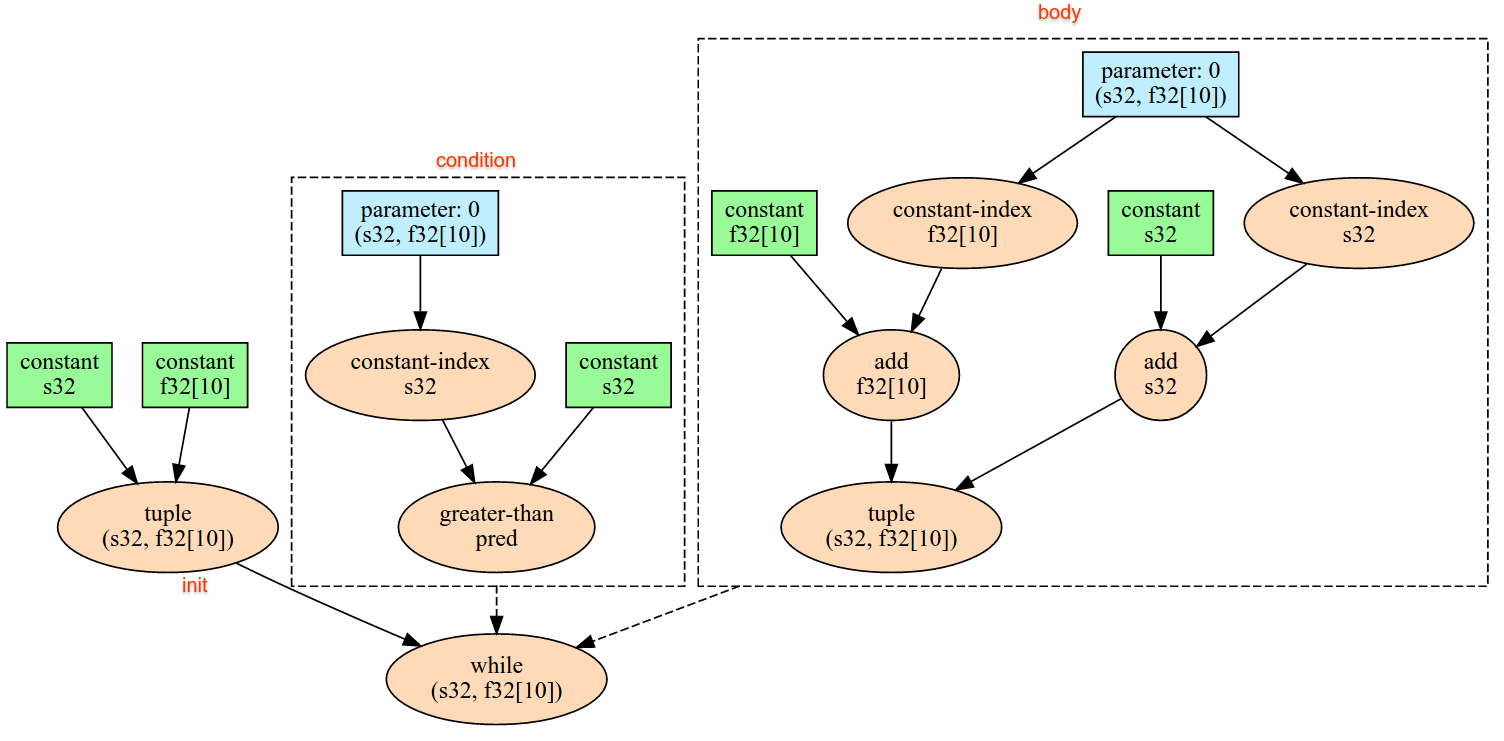
یک مورد داده واحد را از رابط جریان ضمنی infeed دستگاه می خواند ، داده ها را به عنوان شکل داده شده و طرح آن تفسیر می کند و یک XlaOp از داده ها را برمی گرداند. عملیات چندگانه عفونی در یک محاسبه مجاز است ، اما باید در بین عملیات غیرقانونی یک ترتیب کامل وجود داشته باشد. به عنوان مثال ، دو عفونی در کد زیر یک سفارش کلی دارند زیرا بین حلقه های در حالی که وابستگی وجود دارد.
result1 = while (condition, init = init_value) {
  Infeed(shape)
}

result2 = while (condition, init = result1) {
  Infeed(shape)
}
اشکال توله تو در تو در تو پشتیبانی نمی شود. برای یک شکل خالی خالی ، عملیات infeed به طور موثری بدون OP است و بدون خواندن اطلاعاتی از مواد مخدر از دستگاه ، ادامه می یابد.
آیوتا
همچنین به XlaBuilder::Iota مراجعه کنید.
Iota(shape, iota_dimension)
به جای انتقال میزبان بالقوه بزرگ ، یک تحت اللفظی ثابت در دستگاه ایجاد می کند. آرایه ای را ایجاد می کند که شکل مشخص شده و مقادیر را از صفر شروع کرده و توسط یک در طول بعد مشخص شده افزایش می یابد. برای انواع نقطه شناور ، آرایه تولید شده معادل ConvertElementType(Iota(...)) است که Iota از نوع انتگرال است و تبدیل به نوع نقطه شناور است.
| استدلال ها | تایپ کنید | مفاهیم |
|---|---|---|
shape | Shape | شکل آرایه ایجاد شده توسط Iota() |
iota_dimension | int64 | ابعاد افزایش در امتداد. |
به عنوان مثال ، Iota(s32[4, 8], 0) برمی گردد
  [[0, 0, 0, 0, 0, 0, 0, 0 ],
   [1, 1, 1, 1, 1, 1, 1, 1 ],
   [2, 2, 2, 2, 2, 2, 2, 2 ],
   [3, 3, 3, 3, 3, 3, 3, 3 ]]
Iota(s32[4, 8], 1) برمی گردد
  [[0, 1, 2, 3, 4, 5, 6, 7 ],
   [0, 1, 2, 3, 4, 5, 6, 7 ],
   [0, 1, 2, 3, 4, 5, 6, 7 ],
   [0, 1, 2, 3, 4, 5, 6, 7 ]]
نقشه
همچنین به XlaBuilder::Map مراجعه کنید.
Map(operands..., computation)
| استدلال ها | تایپ کنید | مفاهیم |
|---|---|---|
operands | دنباله n XlaOp s | n آرایه های انواع t 0..t {n-1} |
computation | XlaComputation | محاسبه نوع T_0, T_1, .., T_{N + M -1} -> S با پارامترهای N نوع T و M از نوع دلخواه |
dimensions | آرایه int64 | مجموعه ای از ابعاد نقشه |
یک عملکرد مقیاس را بر روی آرایه های operands داده شده اعمال می کند ، و آرایه ای از ابعاد مشابه را تولید می کند که در آن هر عنصر نتیجه عملکرد نقشه برداری شده برای عناصر مربوطه در آرایه های ورودی است.
عملکرد نقشه برداری یک محاسبات دلخواه با محدودیت است که دارای N ورودی از نوع Scalar T و یک خروجی واحد با نوع S است. خروجی ابعاد مشابهی با عملکردها دارد به جز اینکه نوع عنصر t با S. جایگزین می شود
به عنوان مثال: Map(op1, op2, op3, computation, par1) elem_out <- computation(elem1, elem2, elem3, par1) در هر شاخص (چند بعدی) در آرایه های ورودی برای تولید آرایه خروجی نقشه می کند.
بهینه سازی
هرگونه بهینه سازی را از محاسبات متحرک در سد عبور می دهد.
تضمین می کند که تمام ورودی ها قبل از هر اپراتوری که به خروجی سد بستگی دارند ارزیابی می شوند.
پد
همچنین به XlaBuilder::Pad مراجعه کنید.
Pad(operand, padding_value, padding_config)
| استدلال ها | تایپ کنید | مفاهیم |
|---|---|---|
operand | XlaOp | آرایه ای از نوع T |
padding_value | XlaOp | مقیاس T برای پر کردن بالشتک اضافه شده |
padding_config | PaddingConfig | مقدار بالشتک در هر دو لبه (کم ، زیاد) و بین عناصر هر بعد |
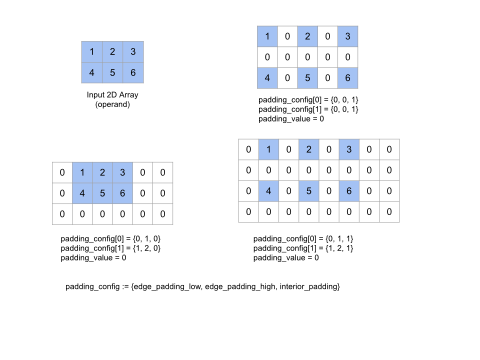
آرایه operand داده شده را با بالشتک در اطراف آرایه و همچنین بین عناصر آرایه با padding_value داده شده گسترش می دهد. padding_config میزان بالشتک لبه و بالشتک داخلی را برای هر بعد مشخص می کند.
PaddingConfig یک میدان مکرر از PaddingConfigDimension است که شامل سه زمینه برای هر بعد است: edge_padding_low ، edge_padding_high و interior_padding .
edge_padding_low و edge_padding_high به ترتیب مقدار بالشتک اضافه شده در سطح پایین (در کنار شاخص 0) و سطح بالا (در کنار بالاترین شاخص) هر بعد را مشخص کنید. مقدار بالشتک لبه می تواند منفی باشد - مقدار مطلق بالشتک منفی تعداد عناصر را برای حذف از بعد مشخص شده نشان می دهد.
interior_padding میزان بالشتک اضافه شده بین هر دو عنصر در هر بعد را مشخص می کند. ممکن است منفی نباشد. بالشتک داخلی به طور منطقی قبل از بالشتک لبه رخ می دهد ، بنابراین در صورت وجود بالشتک لبه منفی ، عناصر از عمل داخلی داخلی خارج می شوند.
این عملیات بدون هیچ گونه OPE است اگر جفت لبه های لبه همه (0 ، 0) و مقادیر بالشتک داخلی همه 0 باشد. شکل زیر نمونه هایی از مقادیر مختلف edge_padding و interior_padding را برای یک آرایه دو بعدی نشان می دهد.
Recv
همچنین به XlaBuilder::Recv مراجعه کنید.
Recv(shape, channel_handle)
| استدلال ها | تایپ کنید | مفاهیم |
|---|---|---|
shape | Shape | شکل داده ها برای دریافت |
channel_handle | ChannelHandle | شناسه منحصر به فرد برای هر جفت ارسال/recv |
داده های شکل داده شده را از یک دستورالعمل Send در یک محاسبات دیگر که همان دسته کانال را به اشتراک می گذارد ، دریافت می کند. یک XLAOP را برای داده های دریافت شده برمی گرداند.
API مشتری از عملیات Recv نشان دهنده ارتباط همزمان است. با این حال ، دستورالعمل در داخل به 2 دستورالعمل HLO ( Recv و RecvDone ) تجزیه می شود تا انتقال داده های ناهمزمان را فعال کند. همچنین به HloInstruction::CreateRecv و HloInstruction::CreateRecvDone مراجعه کنید.
Recv(const Shape& shape, int64 channel_id)
منابع مورد نیاز برای دریافت داده ها را از یک دستورالعمل Send با همان کانال_ید اختصاص می دهد. زمینه ای را برای منابع اختصاص داده شده باز می گرداند ، که توسط یک دستورالعمل RecvDone زیر استفاده می شود تا منتظر تکمیل انتقال داده باشد. متن یک tuple of {دریافت بافر (شکل) ، شناسه درخواست (U32) است و فقط با یک دستورالعمل RecvDone قابل استفاده است.
RecvDone(HloInstruction context)
با توجه به زمینه ای که توسط یک دستورالعمل Recv ایجاد شده است ، منتظر است تا انتقال داده ها تکمیل و داده های دریافت شده را بازگرداند.
كاهش دادن
همچنین به XlaBuilder::Reduce .
یک عملکرد کاهش را به صورت موازی به یک یا چند آرایه اعمال می کند.
Reduce(operands..., init_values..., computation, dimensions)
| استدلال ها | تایپ کنید | مفاهیم |
|---|---|---|
operands | دنباله n XlaOp | n آرایه های انواع T_0, ..., T_{N-1} . |
init_values | دنباله n XlaOp | n مقیاس از انواع T_0, ..., T_{N-1} . |
computation | XlaComputation | محاسبه نوع T_0, ..., T_{N-1}, T_0, ..., T_{N-1} -> Collate(T_0, ..., T_{N-1}) . |
dimensions | آرایه int64 | آرایه ای از ابعاد بدون هماهنگ برای کاهش. |
جایی که:
- n لازم است بیشتر یا برابر با 1 باشد.
- محاسبه باید "تقریباً" انجمنی باشد (به تصویر زیر مراجعه کنید).
- تمام آرایه های ورودی باید ابعاد یکسانی داشته باشند.
- تمام مقادیر اولیه باید تحت
computationهویت تشکیل دهند. - اگر
N = 1،Collate(T)Tاست. - اگر
N > 1،Collate(T_0, ..., T_{N-1})یک قطعه از عناصرNاز نوعTاست.
این عمل یک یا چند بعد از هر آرایه ورودی را به مقیاس ها کاهش می دهد. رتبه هر آرایه برگشتی rank(operand) - len(dimensions) است. خروجی OP Collate(Q_0, ..., Q_N) که در آن Q_i مجموعه ای از نوع T_i است که ابعاد آن در زیر شرح داده شده است.
باکترهای مختلف مجاز به ارتباط مجدد محاسبات کاهش هستند. این می تواند به تفاوت های عددی منجر شود ، زیرا برخی از کارکردهای کاهش مانند علاوه بر این برای شناور نیستند. با این حال ، اگر دامنه داده ها محدود باشد ، اضافه کردن نقطه شناور به اندازه کافی نزدیک است که برای بیشتر مصارف عملی انجمنی باشد.
مثال ها
هنگام کاهش در یک بعد در یک آرایه 1D واحد با مقادیر [10, 11, 12, 13] ، با عملکرد کاهش f (این computation است) سپس می تواند محاسبه شود
f(10, f(11, f(12, f(init_value, 13)))
اما بسیاری از امکانات دیگر نیز وجود دارد ، به عنوان مثال
f(init_value, f(f(10, f(init_value, 11)), f(f(init_value, 12), f(init_value, 13))))
در زیر یک نمونه شبه شبه خشن از نحوه اجرای کاهش ، با استفاده از جمع بندی به عنوان محاسبه کاهش با مقدار اولیه 0 است.
result_shape <- remove all dims in dimensions from operand_shape

# Iterate over all elements in result_shape. The number of r's here is equal
# to the rank of the result
for r0 in range(result_shape[0]), r1 in range(result_shape[1]), ...:
  # Initialize this result element
  result[r0, r1...] <- 0

  # Iterate over all the reduction dimensions
  for d0 in range(dimensions[0]), d1 in range(dimensions[1]), ...:
    # Increment the result element with the value of the operand's element.
    # The index of the operand's element is constructed from all ri's and di's
    # in the right order (by construction ri's and di's together index over the
    # whole operand shape).
    result[r0, r1...] += operand[ri... di]
در اینجا نمونه ای از کاهش یک آرایه 2D (ماتریس) آورده شده است. شکل دارای رتبه 2 ، ابعاد 0 از اندازه 2 و ابعاد 1 اندازه 3 است:
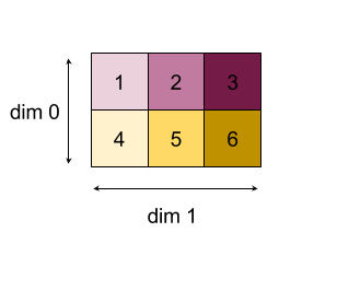
نتایج کاهش ابعاد 0 یا 1 با عملکرد "افزودن":
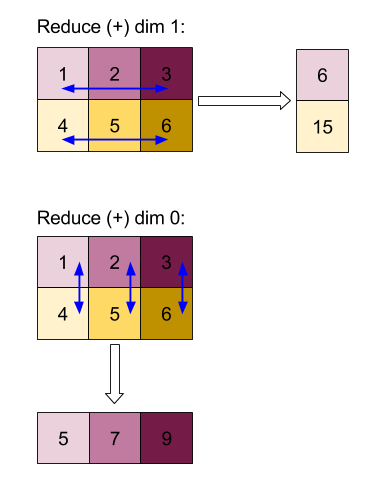
توجه داشته باشید که هر دو نتیجه کاهش آرایه 1D هستند. نمودار یکی را به عنوان ستون و دیگری به عنوان ردیف فقط برای راحتی بصری نشان می دهد.
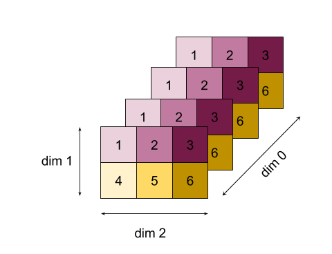
برای مثال پیچیده تر ، در اینجا یک آرایه سه بعدی وجود دارد. رتبه آن 3 ، ابعاد 0 از اندازه 4 ، ابعاد اندازه 2 و ابعاد 2 اندازه 3 است. برای سادگی ، مقادیر 1 تا 6 در ابعاد 0 تکرار می شوند.
به طور مشابه با مثال 2D ، ما می توانیم فقط یک بعد را کاهش دهیم. به عنوان مثال اگر ابعاد 0 را کاهش دهیم ، یک آرایه رتبه 2 را دریافت می کنیم که تمام مقادیر در ابعاد 0 در یک مقیاس قرار گرفتند:
|  4   8  12 |
| 16  20  24 |
اگر ابعاد 2 را کاهش دهیم ، ما یک آرایه رتبه 2 نیز می گیریم که تمام مقادیر در ابعاد 2 در یک مقیاس قرار گرفتند:
| 6  15 |
| 6  15 |
| 6  15 |
| 6  15 |
توجه داشته باشید که ترتیب نسبی بین ابعاد باقیمانده در ورودی در خروجی حفظ می شود ، اما برخی از ابعاد ممکن است اعداد جدیدی را اختصاص دهند (از آنجا که رتبه تغییر می کند).
ما همچنین می توانیم چندین بعد کاهش دهیم. ابعاد کاهش افزودنی 0 و 1 آرایه 1D را تولید می کند [20, 28, 36] .
کاهش آرایه سه بعدی در تمام ابعاد آن ، مقیاس 84 را تولید می کند.
وارییدیک کاهش
هنگامی که N > 1 ، کاهش کاربرد عملکرد کمی پیچیده تر است ، زیرا همزمان در تمام ورودی ها اعمال می شود. عملیات به ترتیب زیر به محاسبات عرضه می شود:
- در حال اجرا مقدار کاهش یافته برای اولین عمل
- ...
- در حال اجرا مقدار کاهش یافته برای عملیات N'TH
- مقدار ورودی برای اولین عمل
- ...
- مقدار ورودی برای عملیات N'TH
به عنوان مثال ، عملکرد کاهش زیر را در نظر بگیرید ، که می تواند برای محاسبه حداکثر و argmax یک آرایه 1-D به طور موازی استفاده شود:
f: (Float, Int, Float, Int) -> Float, Int
f(max, argmax, value, index):
  if value >= max:
    return (value, index)
  else:
    return (max, argmax)
برای آرایه های ورودی 1-D V = Float[N], K = Int[N] ، و مقادیر اولیه I_V = Float, I_K = Int ، نتیجه f_(N-1) کاهش در ابعاد تنها ورودی معادل با برنامه بازگشتی زیر:
f_0 = f(I_V, I_K, V_0, K_0)
f_1 = f(f_0.first, f_0.second, V_1, K_1)
...
f_(N-1) = f(f_(N-2).first, f_(N-2).second, V_(N-1), K_(N-1))
با استفاده از این کاهش در مجموعه ای از مقادیر ، و مجموعه ای از شاخص های پی در پی (IE IOTA) ، بر روی آرایه ها همزمان می شود و یک تاپل حاوی حداکثر مقدار و شاخص تطبیق را باز می گرداند.
کاهش ویژگی
همچنین به XlaBuilder::ReducePrecision مراجعه کنید.
تأثیر تبدیل مقادیر نقطه شناور به فرمت با دقت پایین (مانند IEEE-FP16) و بازگشت به قالب اصلی. تعداد بیت های نماینده و Mantissa در قالب با دقت پایین می تواند به طور خودسرانه مشخص شود ، اگرچه ممکن است تمام اندازه بیت در تمام پیاده سازی های سخت افزاری پشتیبانی نشود.
ReducePrecision(operand, mantissa_bits, exponent_bits)
| استدلال ها | تایپ کنید | مفاهیم |
|---|---|---|
operand | XlaOp | آرایه ای از نوع نقطه شناور T . |
exponent_bits | int32 | تعداد بیت های نماینده در قالب با دقت پایین |
mantissa_bits | int32 | تعداد بیت های مانتیسا در قالب با دقت پایین |
نتیجه آرایه ای از نوع T است. مقادیر ورودی به نزدیکترین مقدار قابل نمایش با تعداد مشخصی از بیت های مانتیسا (با استفاده از معانی "حتی" حتی ") و هر مقداری که بیش از دامنه مشخص شده توسط تعداد بیت های نمایشی باشد ، به بی نهایت مثبت یا منفی می چسبند. مقادیر NaN حفظ می شوند ، اگرچه ممکن است به مقادیر متعارف NaN تبدیل شوند.
قالب با دقت پایین باید حداقل یک بیت نماینده داشته باشد (برای تشخیص مقدار صفر از بی نهایت ، زیرا هر دو دارای یک مانتیسا صفر هستند) و باید تعداد غیر منفی از بیت های مانتیسا داشته باشند. تعداد بیت های نماینده یا Mantissa ممکن است از مقدار مربوطه برای نوع T فراتر رود. بخش مربوط به تبدیل به سادگی یک OP است.
کاسته
همچنین به XlaBuilder::ReduceScatter مراجعه کنید.
RuduceScatter یک عمل جمعی است که به طور مؤثر یک Allreduce را انجام می دهد و سپس با تقسیم آن به بلوک های shard_count در امتداد scatter_dimension و Replica i در گروه Replica ، ith را دریافت می کند.
ReduceScatter(operand, computation, scatter_dim, shard_count, replica_group_ids, channel_id)
| استدلال ها | تایپ کنید | مفاهیم |
|---|---|---|
operand | XlaOp | آرایه یا یک آرایه غیر خالی برای کاهش ماکت ها. |
computation | XlaComputation | محاسبات کاهش |
scatter_dimension | int64 | بعد برای پراکندگی. |
shard_count | int64 | تعداد بلوک ها برای تقسیم scatter_dimension |
replica_groups | بردار بردارهای int64 | گروه هایی که بین آنها کاهش می یابد |
channel_id | اختیاری int64 | شناسه کانال اختیاری برای ارتباط متقابل ماژول |
- هنگامی که
operandیک آرایه از آرایه ها است ، پراکندگی کاهش بر روی هر عنصر Tuple انجام می شود. -
replica_groupsلیستی از گروه های ماکت است که بین آنها کاهش می یابد (شناسه ماکت برای ماکت فعلی می تواند با استفاده ازReplicaIdبازیابی شود). ترتیب ماکت ها در هر گروه ترتیب ترتیب پراکنده شدن نتیجه تمام کاهش را تعیین می کند.replica_groupsیا باید خالی باشد (در این صورت همه ماکت ها متعلق به یک گروه واحد هستند) ، یا حاوی همان تعداد عناصر به عنوان تعداد ماکت ها هستند. هنگامی که بیش از یک گروه ماکت وجود دارد ، همه آنها باید از یک اندازه باشند. به عنوان مثال ،replica_groups = {0, 2}, {1, 3}کاهش بین ماکت های0و2و1و3را انجام می دهد و سپس نتیجه را پراکنده می کند. -
shard_countاندازه هر گروه ماکت است. ما در مواردی کهreplica_groupsخالی هستند ، به این نیاز داریم. اگرreplica_groupsخالی نباشند ،shard_countباید برابر با اندازه هر گروه ماکت باشد. -
channel_idبرای ارتباطات متقابل ماژول استفاده می شود: فقط عملیاتreduce-scatterبا همانchannel_idمی تواند با یکدیگر ارتباط برقرار کند.
شکل خروجی شکل ورودی با scatter_dimension ساخته شده shard_count Times کوچکتر است. به عنوان مثال ، اگر دو ماکت وجود داشته باشد و عملگر دارای مقدار [1.0, 2.25] و [3.0, 5.25] به ترتیب در دو ماکت باشد ، سپس مقدار خروجی از این OP که در آن scatter_dim 0 خواهد بود [4.0] برای اولین بار خواهد بود ماکت و [7.5] برای ماکت دوم.
Window را کاهش دهید
همچنین به XlaBuilder::ReduceWindow مراجعه کنید.
یک تابع کاهش را برای همه عناصر در هر پنجره از یک دنباله از آرایه های چند بعدی N اعمال می کند ، و یک قطعه قطعه از آرایه های چند بعدی N را به عنوان خروجی تولید می کند. هر آرایه خروجی تعداد عناصر مشابهی با تعداد موقعیت های معتبر پنجره دارد. یک لایه استخر را می توان به عنوان یک ReduceWindow بیان کرد. مشابه Reduce ، computation کاربردی همیشه در سمت چپ init_values منتقل می شود.
ReduceWindow(operands..., init_values..., computation, window_dimensions, window_strides, padding)
| استدلال ها | تایپ کنید | مفاهیم |
|---|---|---|
operands | N XlaOps | دنباله ای از آرایه های چند بعدی N از انواع T_0,..., T_{N-1} ، هر کدام نمایانگر ناحیه پایه ای هستند که پنجره روی آن قرار گرفته است. |
init_values | N XlaOps | مقادیر شروع N برای کاهش ، یکی برای هر یک از عملیات N. برای جزئیات بیشتر به کاهش مراجعه کنید. |
computation | XlaComputation | عملکرد کاهش نوع T_0, ..., T_{N-1}, T_0, ..., T_{N-1} -> Collate(T_0, ..., T_{N-1}) برای اعمال در عناصر در هر پنجره از تمام عملیات ورودی. |
window_dimensions | ArraySlice<int64> | آرایه عدد صحیح برای مقادیر ابعاد پنجره |
window_strides | ArraySlice<int64> | مجموعه ای از اعداد صحیح برای مقادیر قدم پنجره |
base_dilations | ArraySlice<int64> | آرایه اعداد صحیح برای مقادیر اتساع پایه |
window_dilations | ArraySlice<int64> | آرایه اعداد صحیح برای مقادیر اتساع پنجره |
padding | Padding | نوع بالشتک برای پنجره (بالشتک :: ksame ، که به گونه ای است که اگر قدم 1 باشد ، شکل خروجی یکسان را دارد ، یا padding :: kvalid ، که از بدون استفاده از بالشتک استفاده می کند و یک بار دیگر پنجره را متوقف نمی کند) |
جایی که:
- n لازم است بیشتر یا برابر با 1 باشد.
- تمام آرایه های ورودی باید ابعاد یکسانی داشته باشند.
- اگر
N = 1،Collate(T)Tاست. - اگر
N > 1،Collate(T_0, ..., T_{N-1})یک قطعه از عناصرNاز نوع(T0,...T{N-1})است.
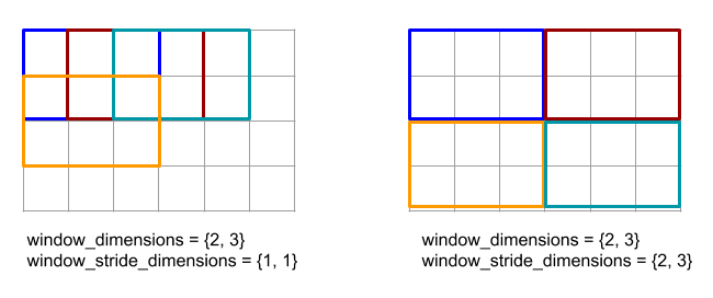
در زیر کد و شکل نمونه ای از استفاده از ReduceWindow را نشان می دهد. ورودی یک ماتریس با اندازه است [4x6] و هر دو Window_Dimensions و Window_Stride_dimensions [2x3] هستند.
// Create a computation for the reduction (maximum).
XlaComputation max;
{
  XlaBuilder builder(client_, "max");
  auto y = builder.Parameter(0, ShapeUtil::MakeShape(F32, {}), "y");
  auto x = builder.Parameter(1, ShapeUtil::MakeShape(F32, {}), "x");
  builder.Max(y, x);
  max = builder.Build().value();
}

// Create a ReduceWindow computation with the max reduction computation.
XlaBuilder builder(client_, "reduce_window_2x3");
auto shape = ShapeUtil::MakeShape(F32, {4, 6});
auto input = builder.Parameter(0, shape, "input");
builder.ReduceWindow(
    input,
    /*init_val=*/builder.ConstantLiteral(LiteralUtil::MinValue(F32)),
    *max,
    /*window_dimensions=*/{2, 3},
    /*window_stride_dimensions=*/{2, 3},
    Padding::kValid);
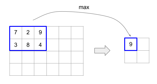
Stride of 1 در یک بعد مشخص می کند که موقعیت یک پنجره در ابعاد 1 عنصر دور از پنجره مجاور آن است. به منظور مشخص کردن که هیچ ویندوز با یکدیگر همپوشانی ندارد ، window_stride_dimensions باید برابر با Window_Dimensions باشد. شکل زیر استفاده از دو مقدار قدم متفاوت را نشان می دهد. بالشتک برای هر بعد از ورودی اعمال می شود و محاسبات همان است که هرچه ورودی با ابعاد موجود پس از بالشتک وارد شود.
For a non-trivial padding example, consider computing reduce-window minimum (initial value is MAX_FLOAT ) with dimension 3 and stride 2 over the input array [10000, 1000, 100, 10, 1] . Padding kValid computes minimums over two valid windows: [10000, 1000, 100] and [100, 10, 1] , resulting in the output [100, 1] . Padding kSame first pads the array so that the shape after the reduce-window would be the same as input for stride one by adding initial elements on both sides, getting [MAX_VALUE, 10000, 1000, 100, 10, 1, MAX_VALUE] . Running reduce-window over the padded array operates on three windows [MAX_VALUE, 10000, 1000] , [1000, 100, 10] , [10, 1, MAX_VALUE] , and yields [1000, 10, 1] .
The evaluation order of the reduction function is arbitrary and may be non-deterministic. Therefore, the reduction function should not be overly sensitive to reassociation. See the discussion about associativity in the context of Reduce for more details.
ReplicaId
See also XlaBuilder::ReplicaId .
Returns the unique ID (U32 scalar) of the replica.
ReplicaId()
The unique ID of each replica is an unsigned integer in the interval [0, N) , where N is the number of replicas. Since all the replicas are running the same program, a ReplicaId() call in the program will return a different value on each replica.
تغییر شکل دهید
See also XlaBuilder::Reshape and the Collapse operation.
Reshapes the dimensions of an array into a new configuration.
Reshape(operand, new_sizes) Reshape(operand, dimensions, new_sizes)
| استدلال ها | تایپ کنید | مفاهیم |
|---|---|---|
operand | XlaOp | array of type T |
dimensions | int64 vector | order in which dimensions are collapsed |
new_sizes | int64 vector | vector of sizes of new dimensions |
Conceptually, reshape first flattens an array into a one-dimensional vector of data values, and then refines this vector into a new shape. The input arguments are an arbitrary array of type T, a compile-time-constant vector of dimension indices, and a compile-time-constant vector of dimension sizes for the result. The values in the dimension vector, if given, must be a permutation of all of T's dimensions; the default if not given is {0, ..., rank - 1} . The order of the dimensions in dimensions is from slowest-varying dimension (most major) to fastest-varying dimension (most minor) in the loop nest which collapses the input array into a single dimension. The new_sizes vector determines the size of the output array. The value at index 0 in new_sizes is the size of dimension 0, the value at index 1 is the size of dimension 1, and so on. The product of the new_size dimensions must equal the product of the operand's dimension sizes. When refining the collapsed array into the multidimensional array defined by new_sizes , the dimensions in new_sizes are ordered from slowest varying (most major) and to fastest varying (most minor).
For example, let v be an array of 24 elements:
let v = f32[4x2x3] { { {10, 11, 12}, {15, 16, 17} },
                    { {20, 21, 22}, {25, 26, 27} },
                    { {30, 31, 32}, {35, 36, 37} },
                    { {40, 41, 42}, {45, 46, 47} } };

In-order collapse:
let v012_24 = Reshape(v, {0,1,2}, {24});
then v012_24 == f32[24] {10, 11, 12, 15, 16, 17, 20, 21, 22, 25, 26, 27,
                         30, 31, 32, 35, 36, 37, 40, 41, 42, 45, 46, 47};

let v012_83 = Reshape(v, {0,1,2}, {8,3});
then v012_83 == f32[8x3] { {10, 11, 12}, {15, 16, 17},
                          {20, 21, 22}, {25, 26, 27},
                          {30, 31, 32}, {35, 36, 37},
                          {40, 41, 42}, {45, 46, 47} };

Out-of-order collapse:
let v021_24 = Reshape(v, {1,2,0}, {24});
then v012_24 == f32[24]  {10, 20, 30, 40, 11, 21, 31, 41, 12, 22, 32, 42,
                          15, 25, 35, 45, 16, 26, 36, 46, 17, 27, 37, 47};

let v021_83 = Reshape(v, {1,2,0}, {8,3});
then v021_83 == f32[8x3] { {10, 20, 30}, {40, 11, 21},
                          {31, 41, 12}, {22, 32, 42},
                          {15, 25, 35}, {45, 16, 26},
                          {36, 46, 17}, {27, 37, 47} };


let v021_262 = Reshape(v, {1,2,0}, {2,6,2});
then v021_262 == f32[2x6x2] { { {10, 20}, {30, 40},
                              {11, 21}, {31, 41},
                              {12, 22}, {32, 42} },
                             { {15, 25}, {35, 45},
                              {16, 26}, {36, 46},
                              {17, 27}, {37, 47} } };
As a special case, reshape can transform a single-element array to a scalar and vice versa. مثلا،
Reshape(f32[1x1] { {5} }, {0,1}, {}) == 5;
Reshape(5, {}, {1,1}) == f32[1x1] { {5} };
Rev (reverse)
See also XlaBuilder::Rev .
Rev(operand, dimensions)
| استدلال ها | تایپ کنید | مفاهیم |
|---|---|---|
operand | XlaOp | array of type T |
dimensions | ArraySlice<int64> | dimensions to reverse |
Reverses the order of elements in the operand array along the specified dimensions , generating an output array of the same shape. Each element of the operand array at a multidimensional index is stored into the output array at a transformed index. The multidimensional index is transformed by reversing the index in each dimension to be reversed (ie, if a dimension of size N is one of the reversing dimensions, its index i is transformed into N - 1 - i).
One use for the Rev operation is to reverse the convolution weight array along the two window dimensions during the gradient computation in neural networks.
RngNormal
See also XlaBuilder::RngNormal .
Constructs an output of a given shape with random numbers generated following the \(N(\mu, \sigma)\) normal distribution. The parameters \(\mu\) and \(\sigma\), and output shape have to have a floating point elemental type. The parameters furthermore have to be scalar valued.
RngNormal(mu, sigma, shape)
| استدلال ها | تایپ کنید | مفاهیم |
|---|---|---|
mu | XlaOp | Scalar of type T specifying mean of generated numbers |
sigma | XlaOp | Scalar of type T specifying standard deviation of generated |
shape | Shape | Output shape of type T |
RngUniform
See also XlaBuilder::RngUniform .
Constructs an output of a given shape with random numbers generated following the uniform distribution over the interval \([a,b)\). The parameters and output element type have to be a boolean type, an integral type or a floating point types, and the types have to be consistent. The CPU and GPU backends currently only support F64, F32, F16, BF16, S64, U64, S32 and U32. Furthermore, the parameters need to be scalar valued. If \(b <= a\) the result is implementation-defined.
RngUniform(a, b, shape)
| استدلال ها | تایپ کنید | مفاهیم |
|---|---|---|
a | XlaOp | Scalar of type T specifying lower limit of interval |
b | XlaOp | Scalar of type T specifying upper limit of interval |
shape | Shape | Output shape of type T |
RngBitGenerator
Generates an output with a given shape filled with uniform random bits using the specified algorithm (or backend default) and returns an updated state (with the same shape as initial state) and the generated random data.
Initial state is the initial state of the current random number generation. It and the required shape and valid values are dependent on the algorithm used.
The output is guaranteed to be a deterministic function of the initial state but it is not guaranteed to be deterministic between backends and different compiler versions.
RngBitGenerator(algorithm, key, shape)
| استدلال ها | تایپ کنید | مفاهیم |
|---|---|---|
algorithm | RandomAlgorithm | PRNG algorithm to be used. |
initial_state | XlaOp | Initial state for the PRNG algorithm. |
shape | Shape | Output shape for generated data. |
Available values for algorithm :
rng_default: Backend specific algorithm with backend specific shape requirements.rng_three_fry: ThreeFry counter-based PRNG algorithm. Theinitial_stateshape isu64[2]with arbitrary values. سالمون و همکاران SC 2011. Parallel random numbers: as easy as 1, 2, 3.rng_philox: Philox algorithm to generate random numbers in parallel. Theinitial_stateshape isu64[3]with arbitrary values. سالمون و همکاران SC 2011. Parallel random numbers: as easy as 1, 2, 3.
پراکنده کردن
The XLA scatter operation generates a sequence of results which are the values of the input array operands , with several slices (at indices specified by scatter_indices ) updated with the sequence of values in updates using update_computation .
See also XlaBuilder::Scatter .
scatter(operands..., scatter_indices, updates..., update_computation, index_vector_dim, update_window_dims, inserted_window_dims, scatter_dims_to_operand_dims)
| استدلال ها | تایپ کنید | مفاهیم |
|---|---|---|
operands | Sequence of N XlaOp | N arrays of types T_0, ..., T_N to be scattered into. |
scatter_indices | XlaOp | Array containing the starting indices of the slices that must be scattered to. |
updates | Sequence of N XlaOp | N arrays of types T_0, ..., T_N . updates[i] contains the values that must be used for scattering operands[i] . |
update_computation | XlaComputation | Computation to be used for combining the existing values in the input array and the updates during scatter. This computation should be of type T_0, ..., T_N, T_0, ..., T_N -> Collate(T_0, ..., T_N) . |
index_vector_dim | int64 | The dimension in scatter_indices that contains the starting indices. |
update_window_dims | ArraySlice<int64> | The set of dimensions in updates shape that are window dimensions . |
inserted_window_dims | ArraySlice<int64> | The set of window dimensions that must be inserted into updates shape. |
scatter_dims_to_operand_dims | ArraySlice<int64> | A dimensions map from the scatter indices to the operand index space. This array is interpreted as mapping i to scatter_dims_to_operand_dims[i] . It has to be one-to-one and total. |
indices_are_sorted | bool | Whether the indices are guaranteed to be sorted by the caller. |
جایی که:
- N is required to be greater or equal to 1.
-
operands[0], ...,operands[N-1] must all have the same dimensions. -
updates[0], ...,updates[N-1] must all have the same dimensions. - If
N = 1,Collate(T)isT. - If
N > 1,Collate(T_0, ..., T_N)is a tuple ofNelements of typeT.
If index_vector_dim is equal to scatter_indices.rank we implicitly consider scatter_indices to have a trailing 1 dimension.
We define update_scatter_dims of type ArraySlice<int64> as the set of dimensions in updates shape that are not in update_window_dims , in ascending order.
The arguments of scatter should follow these constraints:
Each
updatesarray must be of rankupdate_window_dims.size + scatter_indices.rank - 1.Bounds of dimension
iin eachupdatesarray must conform to the following:- If
iis present inupdate_window_dims(ie equal toupdate_window_dims[k] for somek), then the bound of dimensioniinupdatesmust not exceed the corresponding bound ofoperandafter accounting for theinserted_window_dims(ieadjusted_window_bounds[k], whereadjusted_window_boundscontains the bounds ofoperandwith the bounds at indicesinserted_window_dimsremoved). - If
iis present inupdate_scatter_dims(ie equal toupdate_scatter_dims[k] for somek), then the bound of dimensioniinupdatesmust be equal to the corresponding bound ofscatter_indices, skippingindex_vector_dim(iescatter_indices.shape.dims[k], ifk<index_vector_dimandscatter_indices.shape.dims[k+1] otherwise).
- If
update_window_dimsmust be in ascending order, not have any repeating dimension numbers, and be in the range[0, updates.rank).inserted_window_dimsmust be in ascending order, not have any repeating dimension numbers, and be in the range[0, operand.rank).operand.rankmust equal the sum ofupdate_window_dims.sizeandinserted_window_dims.size.scatter_dims_to_operand_dims.sizemust be equal toscatter_indices.shape.dims[index_vector_dim], and its values must be in the range[0, operand.rank).
For a given index U in each updates array, the corresponding index I in the corresponding operands array into which this update has to be applied is computed as follows:
- Let
G= {U[k] forkinupdate_scatter_dims}. UseGto look up an index vectorSin thescatter_indicesarray such thatS[i] =scatter_indices[Combine(G,i)] where Combine(A, b) inserts b at positionsindex_vector_diminto A. - Create an index
SinintooperandusingSby scatteringSusing thescatter_dims_to_operand_dimsmap. رسمی تر:-
Sin[scatter_dims_to_operand_dims[k]] =S[k] ifk<scatter_dims_to_operand_dims.size. -
Sin[_] =0otherwise.
-
- Create an index
Wininto eachoperandsarray by scattering the indices atupdate_window_dimsinUaccording toinserted_window_dims. رسمی تر:-
Win[window_dims_to_operand_dims(k)] =U[k] ifkis inupdate_window_dims, wherewindow_dims_to_operand_dimsis the monotonic function with domain [0,update_window_dims.size) and range [0,operand.rank) \inserted_window_dims. (For example, ifupdate_window_dims.sizeis4,operand.rankis6, andinserted_window_dimsis {0,2} thenwindow_dims_to_operand_dimsis {0→1,1→3,2→4,3→5}). -
Win[_] =0otherwise.
-
-
IisWin+Sinwhere + is element-wise addition.
In summary, the scatter operation can be defined as follows.
- Initialize
outputwithoperands, ie for all indicesJ, for all indicesOin theoperands[J] array:
output[J][O] =operands[J][O] - For every index
Uin theupdates[J] array and the corresponding indexOin theoperand[J] array, ifOis a valid index foroutput:
(output[0][O], ...,output[N-1][O]) =update_computation(output[0][O], ..., ,output[N-1][O],updates[0][U], ...,updates[N-1][U])
The order in which updates are applied is non-deterministic. So, when multiple indices in updates refer to the same index in operands , the corresponding value in output will be non-deterministic.
Note that the first parameter that is passed into the update_computation will always be the current value from the output array and the second parameter will always be the value from the updates array. This is important specifically for cases when the update_computation is not commutative .
If indices_are_sorted is set to true then XLA can assume that start_indices are sorted (in ascending start_index_map order) by the user. If they are not then the semantics is implementation defined.
Informally, the scatter op can be viewed as an inverse of the gather op, ie the scatter op updates the elements in the input that are extracted by the corresponding gather op.
For a detailed informal description and examples, refer to the "Informal Description" section under Gather .
انتخاب کنید
See also XlaBuilder::Select .
Constructs an output array from elements of two input arrays, based on the values of a predicate array.
Select(pred, on_true, on_false)
| استدلال ها | تایپ کنید | مفاهیم |
|---|---|---|
pred | XlaOp | array of type PRED |
on_true | XlaOp | array of type T |
on_false | XlaOp | array of type T |
The arrays on_true and on_false must have the same shape. This is also the shape of the output array. The array pred must have the same dimensionality as on_true and on_false , with the PRED element type.
For each element P of pred , the corresponding element of the output array is taken from on_true if the value of P is true , and from on_false if the value of P is false . As a restricted form of broadcasting , pred can be a scalar of type PRED . In this case, the output array is taken wholly from on_true if pred is true , and from on_false if pred is false .
Example with non-scalar pred :
let pred: PRED[4] = {true, false, false, true};
let v1: s32[4] = {1, 2, 3, 4};
let v2: s32[4] = {100, 200, 300, 400};
==>
Select(pred, v1, v2) = s32[4]{1, 200, 300, 4};
Example with scalar pred :
let pred: PRED = true;
let v1: s32[4] = {1, 2, 3, 4};
let v2: s32[4] = {100, 200, 300, 400};
==>
Select(pred, v1, v2) = s32[4]{1, 2, 3, 4};
Selections between tuples are supported. Tuples are considered to be scalar types for this purpose. If on_true and on_false are tuples (which must have the same shape!) then pred has to be a scalar of type PRED .
SelectAndScatter
See also XlaBuilder::SelectAndScatter .
This operation can be considered as a composite operation that first computes ReduceWindow on the operand array to select an element from each window, and then scatters the source array to the indices of the selected elements to construct an output array with the same shape as the operand آرایه. The binary select function is used to select an element from each window by applying it across each window, and it is called with the property that the first parameter's index vector is lexicographically less than the second parameter's index vector. The select function returns true if the first parameter is selected and returns false if the second parameter is selected, and the function must hold transitivity (ie, if select(a, b) and select(b, c) are true , then select(a, c) is also true ) so that the selected element does not depend on the order of the elements traversed for a given window.
The function scatter is applied at each selected index in the output array. It takes two scalar parameters:
- Current value at the selected index in the output array
- The scatter value from
sourcethat applies to the selected index
It combines the two parameters and returns a scalar value that's used to update the value at the selected index in the output array. Initially, all indices of the output array are set to init_value .
The output array has the same shape as the operand array and the source array must have the same shape as the result of applying a ReduceWindow operation on the operand array. SelectAndScatter can be used to backpropagate the gradient values for a pooling layer in a neural network.
SelectAndScatter(operand, select, window_dimensions, window_strides, padding, source, init_value, scatter)
| استدلال ها | تایپ کنید | مفاهیم |
|---|---|---|
operand | XlaOp | array of type T over which the windows slide |
select | XlaComputation | binary computation of type T, T -> PRED , to apply to all elements in each window; returns true if the first parameter is selected and returns false if the second parameter is selected |
window_dimensions | ArraySlice<int64> | array of integers for window dimension values |
window_strides | ArraySlice<int64> | array of integers for window stride values |
padding | Padding | padding type for window (Padding::kSame or Padding::kValid) |
source | XlaOp | array of type T with the values to scatter |
init_value | XlaOp | scalar value of type T for the initial value of the output array |
scatter | XlaComputation | binary computation of type T, T -> T , to apply each scatter source element with its destination element |
The figure below shows examples of using SelectAndScatter , with the select function computing the maximal value among its parameters. Note that when the windows overlap, as in the figure (2) below, an index of the operand array may be selected multiple times by different windows. In the figure, the element of value 9 is selected by both of the top windows (blue and red) and the binary addition scatter function produces the output element of value 8 (2 + 6).
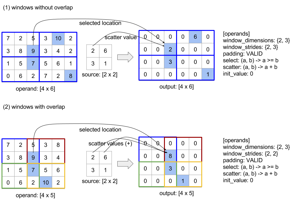
The evaluation order of the scatter function is arbitrary and may be non-deterministic. Therefore, the scatter function should not be overly sensitive to reassociation. See the discussion about associativity in the context of Reduce for more details.
ارسال
See also XlaBuilder::Send .
Send(operand, channel_handle)
| استدلال ها | تایپ کنید | مفاهیم |
|---|---|---|
operand | XlaOp | data to send (array of type T) |
channel_handle | ChannelHandle | unique identifier for each send/recv pair |
Sends the given operand data to a Recv instruction in another computation that shares the same channel handle. Does not return any data.
Similar to the Recv operation, the client API of Send operation represents synchronous communication, and is internally decomposed into 2 HLO instructions ( Send and SendDone ) to enable asynchronous data transfers. See also HloInstruction::CreateSend and HloInstruction::CreateSendDone .
Send(HloInstruction operand, int64 channel_id)
Initiates an asynchronous transfer of the operand to the resources allocated by the Recv instruction with the same channel id. Returns a context, which is used by a following SendDone instruction to wait for the completion of the data transfer. The context is a tuple of {operand (shape), request identifier (U32)} and it can only be used by a SendDone instruction.
SendDone(HloInstruction context)
Given a context created by a Send instruction, waits for the data transfer to complete. The instruction does not return any data.
Scheduling of channel instructions
The execution order of the 4 instructions for each channel ( Recv , RecvDone , Send , SendDone ) is as below.
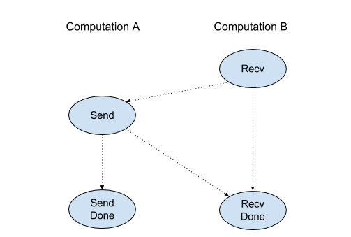
-
Recvhappens beforeSend -
Sendhappens beforeRecvDone -
Recvhappens beforeRecvDone -
Sendhappens beforeSendDone
When the backend compilers generate a linear schedule for each computation that communicates via channel instructions, there must not be cycles across the computations. For example, below schedules lead to deadlocks.
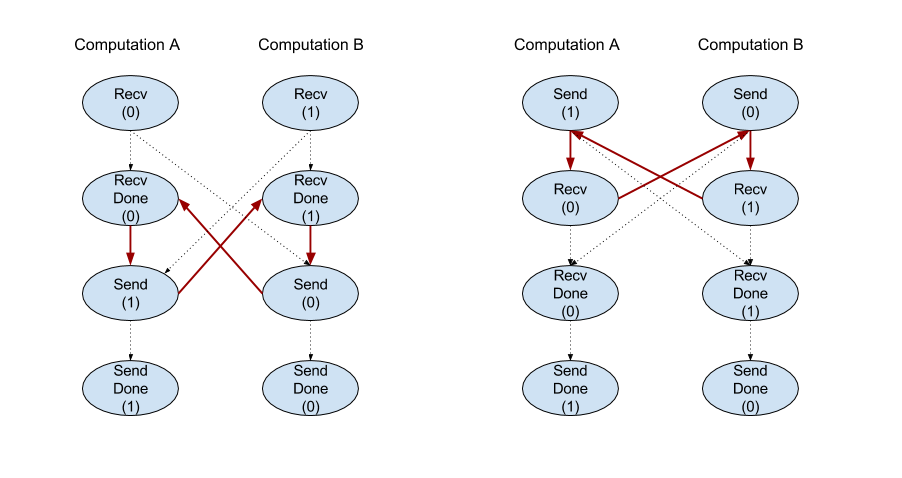
تکه
See also XlaBuilder::Slice .
Slicing extracts a sub-array from the input array. The sub-array is of the same rank as the input and contains the values inside a bounding box within the input array where the dimensions and indices of the bounding box are given as arguments to the slice operation.
Slice(operand, start_indices, limit_indices, strides)
| استدلال ها | تایپ کنید | مفاهیم |
|---|---|---|
operand | XlaOp | N dimensional array of type T |
start_indices | ArraySlice<int64> | List of N integers containing the starting indices of the slice for each dimension. Values must be greater than or equal to zero. |
limit_indices | ArraySlice<int64> | List of N integers containing the ending indices (exclusive) for the slice for each dimension. Each value must be greater than or equal to the respective start_indices value for the dimension and less than or equal to the size of the dimension. |
strides | ArraySlice<int64> | List of N integers that decides the input stride of the slice. The slice picks every strides[d] element in dimension d . |
1-dimensional example:
let a = {0.0, 1.0, 2.0, 3.0, 4.0}
Slice(a, {2}, {4}) produces:
  {2.0, 3.0}
2-dimensional example:
let b =
 { {0.0,  1.0,  2.0},
   {3.0,  4.0,  5.0},
   {6.0,  7.0,  8.0},
   {9.0, 10.0, 11.0} }

Slice(b, {2, 1}, {4, 3}) produces:
  { { 7.0,  8.0},
    {10.0, 11.0} }
مرتب سازی
See also XlaBuilder::Sort .
Sort(operands, comparator, dimension, is_stable)
| استدلال ها | تایپ کنید | مفاهیم |
|---|---|---|
operands | ArraySlice<XlaOp> | The operands to sort. |
comparator | XlaComputation | The comparator computation to use. |
dimension | int64 | The dimension along which to sort. |
is_stable | bool | Whether stable sorting should be used. |
If only one operand is provided:
If the operand is a rank-1 tensor (an array), the result is a sorted array. If you want to sort the array into ascending order, the comparator should perform a less-than comparison. Formally, after the array is sorted, it holds for all index positions
i, jwithi < jthat eithercomparator(value[i], value[j]) = comparator(value[j], value[i]) = falseorcomparator(value[i], value[j]) = true.If the operand has higher rank, the operand is sorted along the provided dimension. For example, for a rank-2 tensor (a matrix), a dimension value of
0will independently sort every column, and a dimension value of1will independently sort each row. If no dimension number is provided, then the last dimension is chosen by default. For the dimension which is sorted, the same sorting order applies as in the rank-1 case.
If n > 1 operands are provided:
All
noperands must be tensors with the same dimensions. The element types of the tensors may be different.All operands are sorted together, not individually. Conceptually the operands are treated as a tuple. When checking whether the elements of each operand at index positions
iandjneed to be swapped, the comparator is called with2 * nscalar parameters, where parameter2 * kcorresponds to the value at positionifrom thek-thoperand, and parameter2 * k + 1corresponds to the value at positionjfrom thek-thoperand. Usually, the comparator would thus compare parameters2 * kand2 * k + 1with each other and possibly use other parameter pairs as tie breakers.The result is a tuple that consists of the operands in sorted order (along the provided dimension, as above). The
i-thoperand of the tuple corresponds to thei-thoperand of Sort.
For example, if there are three operands operand0 = [3, 1] , operand1 = [42, 50] , operand2 = [-3.0, 1.1] , and the comparator compares only the values of operand0 with less-than, then the output of the sort is the tuple ([1, 3], [50, 42], [1.1, -3.0]) .
If is_stable is set to true, the sort is guaranteed to be stable, that is, if there are elements which are considered to be equal by the comparator, the relative order of the equal values is preserved. Two elements e1 and e2 are equal if and only if comparator(e1, e2) = comparator(e2, e1) = false . By default, is_stable is set to false.
جابجا شود
See also the tf.reshape operation.
Transpose(operand)
| استدلال ها | تایپ کنید | مفاهیم |
|---|---|---|
operand | XlaOp | The operand to transpose. |
permutation | ArraySlice<int64> | How to permute the dimensions. |
Permutes the operand dimensions with the given permutation, so ∀ i . 0 ≤ i < rank ⇒ input_dimensions[permutation[i]] = output_dimensions[i] .
This is the same as Reshape(operand, permutation, Permute(permutation, operand.shape.dimensions)).
TriangularSolve
See also XlaBuilder::TriangularSolve .
Solves systems of linear equations with lower or upper triangular coefficient matrices by forward- or back-substitution. Broadcasting along leading dimensions, this routine solves one of the matrix systems op(a) * x = b , or x * op(a) = b , for the variable x , given a and b , where op(a) is either op(a) = a , or op(a) = Transpose(a) , or op(a) = Conj(Transpose(a)) .
TriangularSolve(a, b, left_side, lower, unit_diagonal, transpose_a)
| استدلال ها | تایپ کنید | مفاهیم |
|---|---|---|
a | XlaOp | a rank > 2 array of a complex or floating-point type with shape [..., M, M] . |
b | XlaOp | a rank > 2 array of the same type with shape [..., M, K] if left_side is true, [..., K, M] otherwise. |
left_side | bool | indicates whether to solve a system of the form op(a) * x = b ( true ) or x * op(a) = b ( false ). |
lower | bool | whether to use the upper or lower triangle of a . |
unit_diagonal | bool | if true , the diagonal elements of a are assumed to be 1 and not accessed. |
transpose_a | Transpose | whether to use a as is, transpose it or take its conjugate transpose. |
Input data is read only from the lower/upper triangle of a , depending on the value of lower . Values from the other triangle are ignored. Output data is returned in the same triangle; the values in the other triangle are implementation-defined and may be anything.
If the rank of a and b are greater than 2, they are treated as batches of matrices, where all except the minor 2 dimensions are batch dimensions. a and b must have equal batch dimensions.
چندتایی
See also XlaBuilder::Tuple .
A tuple containing a variable number of data handles, each of which has its own shape.
This is analogous to std::tuple in C++. مفهومی:
let v: f32[10] = f32[10]{0, 1, 2, 3, 4, 5, 6, 7, 8, 9};
let s: s32 = 5;
let t: (f32[10], s32) = tuple(v, s);
Tuples can be deconstructed (accessed) via the GetTupleElement operation.
در حالی که
See also XlaBuilder::While .
While(condition, body, init)
| استدلال ها | تایپ کنید | مفاهیم |
|---|---|---|
condition | XlaComputation | XlaComputation of type T -> PRED which defines the termination condition of theloop. |
body | XlaComputation | XlaComputation of type T -> T which defines the body of the loop. |
init | T | Initial value for the parameter of condition and body . |
Sequentially executes the body until the condition fails. This is similar to a typical while loop in many other languages except for the differences and restrictions listed below.
- A
Whilenode returns a value of typeT, which is the result from the last execution of thebody. - The shape of the type
Tis statically determined and must be the same across all iterations.
The T parameters of the computations are initialized with the init value in the first iteration and are automatically updated to the new result from body in each subsequent iteration.
One main use case of the While node is to implement the repeated execution of training in neural networks. Simplified pseudocode is shown below with a graph that represents the computation. The code can be found in while_test.cc . The type T in this example is a Tuple consisting of an int32 for the iteration count and a vector[10] for the accumulator. For 1000 iterations, the loop keeps adding a constant vector to the accumulator.
// Pseudocode for the computation.
init = {0, zero_vector[10]} // Tuple of int32 and float[10].
result = init;
while (result(0) < 1000) {
  iteration = result(0) + 1;
  new_vector = result(1) + constant_vector[10];
  result = {iteration, new_vector};
}