A continuación, se describe la semántica de las operaciones definidas en la interfaz XlaBuilder. Por lo general, estas operaciones se asignan uno a uno a las operaciones definidas en la interfaz de RPC en xla_data.proto.
Nota sobre la nomenclatura: El tipo de datos generalizado con el que se trata XLA es un array de N dimensiones que contiene elementos de algún tipo uniforme (como el número de punto flotante de 32 bits). En toda la documentación, se usa array para denotar un array de dimensiones arbitrarias. Para mayor comodidad, los casos especiales tienen nombres más específicos y conocidos; por ejemplo, un vector es un arreglo unidimensional y una matriz es un arreglo de dos dimensiones.
AfterAll
Consulta también XlaBuilder::AfterAll.
AfterAll toma una cantidad variable de tokens y produce un solo token. Los tokens son tipos primitivos que se pueden agrupar entre operaciones secundarias para aplicar el orden. AfterAll se puede usar como una unión de tokens para ordenar una operación después de una operación de configuración.
AfterAll(operands)
| Argumentos | Tipo | Semántica |
|---|---|---|
operands |
XlaOp |
cantidad variable de tokens |
AllGather
Consulta también XlaBuilder::AllGather.
Realiza la concatenación entre réplicas.
AllGather(operand, all_gather_dim, shard_count, replica_group_ids,
channel_id)
| Argumentos | Tipo | Semántica |
|---|---|---|
operand
|
XlaOp
|
Arreglo para concatenar entre réplicas |
all_gather_dim |
int64 |
Dimensión de concatenación |
replica_groups
|
vector de vectores de int64 |
Los grupos entre los que se realiza la concatenación |
channel_id
|
int64 opcional
|
ID de canal opcional para la comunicación entre módulos |
replica_groupses una lista de grupos de réplica entre los que se realiza la concatenación (el ID de réplica de la réplica actual se puede recuperar medianteReplicaId). El orden de las réplicas en cada grupo determina el orden en el que se ubican sus entradas en el resultado.replica_groupsdebe estar vacío (en ese caso, todas las réplicas pertenecen a un solo grupo, ordenado de0aN - 1) o debe contener la misma cantidad de elementos que la cantidad de réplicas. Por ejemplo,replica_groups = {0, 2}, {1, 3}realiza la concatenación entre las réplicas0y2, y1y3.shard_countes el tamaño de cada grupo de réplicas. Necesitamos esto en los casos en quereplica_groupsesté vacío.channel_idse usa para la comunicación entre módulos: solo las operacionesall-gathercon el mismochannel_idpueden comunicarse entre sí.
La forma de salida es la de entrada con el elemento all_gather_dim hecho shard_count veces más grande. Por ejemplo, si hay dos réplicas y el operando tiene el valor [1.0, 2.5] y [3.0, 5.25] respectivamente en las dos réplicas, el valor de salida de esta operación en la que all_gather_dim es 0 será [1.0, 2.5, 3.0,
5.25] en ambas réplicas.
AllReduce
Consulta también XlaBuilder::AllReduce.
Realiza cálculos personalizados entre réplicas.
AllReduce(operand, computation, replica_group_ids, channel_id)
| Argumentos | Tipo | Semántica |
|---|---|---|
operand
|
XlaOp
|
Arreglo o una tupla no vacía de arreglos para reducir en las réplicas |
computation |
XlaComputation |
Cálculo de la reducción |
replica_groups
|
vector de vectores de int64 |
Los grupos entre los que se realizan las reducciones |
channel_id
|
int64 opcional
|
ID de canal opcional para la comunicación entre módulos |
- Cuando
operandes una tupla de arreglos, la reducción total se realiza en cada elemento de la tupla. replica_groupses una lista de grupos de réplicas entre los que se realiza la reducción (el ID de réplica de la réplica actual se puede recuperar medianteReplicaId).replica_groupsdebe estar vacío (en ese caso, todas las réplicas pertenecen a un solo grupo) o contener la misma cantidad de elementos que la cantidad de réplicas. Por ejemplo,replica_groups = {0, 2}, {1, 3}realiza una reducción entre las réplicas0y2, y entre1y3.channel_idse usa para la comunicación entre módulos: solo las operacionesall-reducecon el mismochannel_idpueden comunicarse entre sí.
La forma de salida es la misma que la de entrada. Por ejemplo, si hay dos réplicas y el operando tiene el valor [1.0, 2.5] y [3.0, 5.25], respectivamente, en las dos réplicas, el valor de salida de este cálculo de operación y suma será [4.0, 7.75] en ambas réplicas. Si la entrada es una tupla, el resultado también es una tupla.
Para calcular el resultado de AllReduce, es necesario tener una entrada de cada réplica, por lo que, si una réplica ejecuta un nodo AllReduce más veces que otra, la réplica anterior esperará por siempre. Dado que todas las réplicas ejecutan el mismo programa, no hay muchas formas para que eso suceda, pero es posible cuando la condición de un bucle while depende de los datos de la entrada y los datos que se ingresan hacen que el bucle while se itere más veces en una réplica que en otra.
AllToAll
Consulta también XlaBuilder::AllToAll.
AllToAll es una operación colectiva que envía datos de todos los núcleos a todos los núcleos. Consta de dos fases:
- Fase de dispersión En cada núcleo, el operando se divide en la cantidad de bloques
split_counta lo largo delsplit_dimensions, y los bloques se dispersan en todos los núcleos, p.ej., el bloque i se envía al núcleo i. - La fase de recopilación. Cada núcleo concatena los bloques recibidos a lo largo de
concat_dimension.
Los núcleos que participan se pueden configurar de la siguiente manera:
replica_groups: Cada ReplicaGroup contiene una lista de los IDs de réplica que participan en el cálculo (el ID de réplica de la réplica actual se puede recuperar conReplicaId). AllToAll se aplicará dentro de los subgrupos en el orden especificado. Por ejemplo,replica_groups = { {1,2,3}, {4,5,0} }significa que se aplicará AllToAll en las réplicas de{1, 2, 3}y, en la fase de recopilación, y los bloques recibidos se concatenarán en el mismo orden de 1, 2, 3. Luego, se aplicará otro AllToAll en las réplicas 4, 5 y 0, y el orden de concatenación también es 4, 5, 0. Sireplica_groupsestá vacío, todas las réplicas pertenecen a un grupo, en el orden de concatenación de su aparición.
Requisitos previos:
- El tamaño de la dimensión del operando en
split_dimensiones divisible porsplit_count. - La forma del operando no es una tupla.
AllToAll(operand, split_dimension, concat_dimension, split_count,
replica_groups)
| Argumentos | Tipo | Semántica |
|---|---|---|
operand |
XlaOp |
array de entrada de n dimensiones |
split_dimension
|
int64
|
Un valor en el intervalo [0,
n) que nombra la dimensión en la que se divide el operando. |
concat_dimension
|
int64
|
Un valor en el intervalo [0,
n) que nombra la dimensión a lo largo de la cual se concatenan los bloques de división |
split_count
|
int64
|
La cantidad de núcleos que participan en esta operación. Si replica_groups está vacío, esta debería ser la cantidad de réplicas; de lo contrario, debería ser igual a la cantidad de réplicas en cada grupo. |
replica_groups
|
Vector de ReplicaGroup
|
Cada grupo contiene una lista de IDs de réplica. |
A continuación, se muestra un ejemplo de Alltoall.
XlaBuilder b("alltoall");
auto x = Parameter(&b, 0, ShapeUtil::MakeShape(F32, {4, 16}), "x");
AllToAll(x, /*split_dimension=*/1, /*concat_dimension=*/0, /*split_count=*/4);
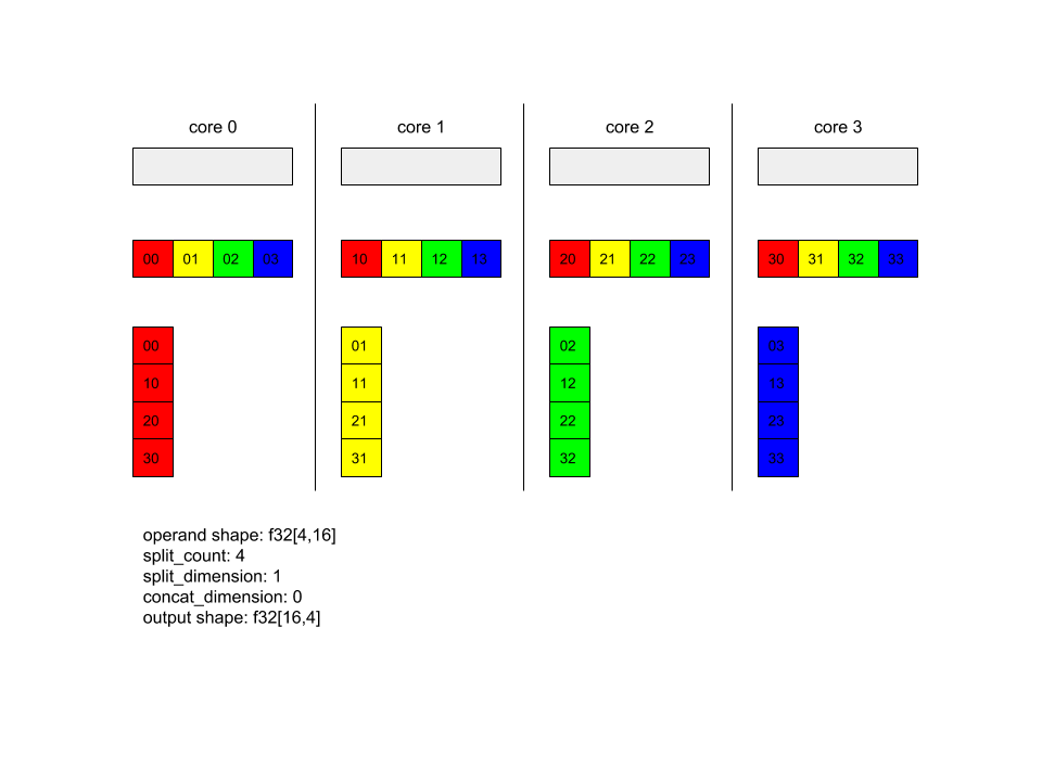
En este ejemplo, hay 4 núcleos que participan en el Alltoall. En cada núcleo, el operando se divide en 4 partes a lo largo de la dimensión 0, por lo que cada parte tiene la forma f32[4,4]. Las 4 partes están dispersas en todos los núcleos. Luego, cada núcleo concatena las partes recibidas en la dimensión 1, en el orden del núcleo 0 a 4. Por lo tanto, el resultado en cada núcleo tiene la forma f32[16,4].
BatchNormGrad
Consulta también XlaBuilder::BatchNormGrad y el documento original de normalización por lotes para obtener una descripción detallada del algoritmo.
Calcula los gradientes de la norma del lote.
BatchNormGrad(operand, scale, mean, variance, grad_output, epsilon, feature_index)
| Argumentos | Tipo | Semántica |
|---|---|---|
operand |
XlaOp |
array de n dimensiones que se normalizará (x) |
scale |
XlaOp |
Array de 1 dimensión (\(\gamma\)) |
mean |
XlaOp |
Array de 1 dimensión (\(\mu\)) |
variance |
XlaOp |
Array de 1 dimensión (\(\sigma^2\)) |
grad_output |
XlaOp |
Gradientes pasados a BatchNormTraining (\(\nabla y\)) |
epsilon |
float |
Valor de épsilon (\(\epsilon\)) |
feature_index |
int64 |
Índice a la dimensión del atributo en operand |
Para cada componente de la dimensión del componente (feature_index es el índice de la dimensión del componente en operand), la operación calcula los gradientes con respecto a operand, offset y scale en todas las demás dimensiones. El feature_index debe ser un índice válido para la dimensión del atributo en operand.
Los tres gradientes se definen con las siguientes fórmulas (suponiendo un array de 4 dimensiones como operand y con el índice de dimensión de atributos l, el tamaño del lote m y los tamaños espaciales w y h):
\[ \begin{split} c_l&= \frac{1}{mwh}\sum_{i=1}^m\sum_{j=1}^w\sum_{k=1}^h \left( \nabla y_{ijkl} \frac{x_{ijkl} - \mu_l}{\sigma^2_l+\epsilon} \right) \\\\ d_l&= \frac{1}{mwh}\sum_{i=1}^m\sum_{j=1}^w\sum_{k=1}^h \nabla y_{ijkl} \\\\ \nabla x_{ijkl} &= \frac{\gamma_{l} }{\sqrt{\sigma^2_{l}+\epsilon} } \left( \nabla y_{ijkl} - d_l - c_l (x_{ijkl} - \mu_{l}) \right) \\\\ \nabla \gamma_l &= \sum_{i=1}^m\sum_{j=1}^w\sum_{k=1}^h \left( \nabla y_{ijkl} \frac{x_{ijkl} - \mu_l}{\sqrt{\sigma^2_{l}+\epsilon} } \right) \\\\\ \nabla \beta_l &= \sum_{i=1}^m\sum_{j=1}^w\sum_{k=1}^h \nabla y_{ijkl} \end{split} \]
Las entradas mean y variance representan valores de momentos en dimensiones por lotes y espaciales.
El tipo de salida es una tupla de tres controladores:
| Salidas | Tipo | Semántica |
|---|---|---|
grad_operand
|
XlaOp
|
gradiente con respecto al operand de entrada ($\nabla x$) |
grad_scale
|
XlaOp
|
gradiente con respecto al scale de entrada ($\nabla
\gamma$) |
grad_offset
|
XlaOp
|
gradiente con respecto a la entrada offset($\nabla \beta$) |
BatchNormInference
Consulta también XlaBuilder::BatchNormInference y el documento original de normalización por lotes para obtener una descripción detallada del algoritmo.
Normaliza un array en dimensiones por lotes y espaciales.
BatchNormInference(operand, scale, offset, mean, variance, epsilon, feature_index)
| Argumentos | Tipo | Semántica |
|---|---|---|
operand |
XlaOp |
array de n dimensiones que se normalizará |
scale |
XlaOp |
Array de 1 dimensión |
offset |
XlaOp |
Array de 1 dimensión |
mean |
XlaOp |
Array de 1 dimensión |
variance |
XlaOp |
Array de 1 dimensión |
epsilon |
float |
Valor de épsilon |
feature_index |
int64 |
Índice a la dimensión del atributo en operand |
Para cada componente de la dimensión del componente (feature_index es el índice de la dimensión del componente en operand), la operación calcula la media y la varianza de todas las demás dimensiones, y usa la media y la varianza para normalizar cada elemento en operand. feature_index debe ser un índice válido para la dimensión del componente en operand.
BatchNormInference equivale a llamar a BatchNormTraining sin procesar mean ni variance para cada lote. En su lugar, usa los elementos de entrada mean y variance como valores estimados. El propósito de esta op es reducir la latencia en la inferencia, de ahí el nombre de BatchNormInference.
El resultado es un arreglo normalizado de n dimensiones con la misma forma que la entrada operand.
BatchNormTraining
Consulta también XlaBuilder::BatchNormTraining y the original batch normalization paper para obtener una descripción detallada del algoritmo.
Normaliza un array en dimensiones por lotes y espaciales.
BatchNormTraining(operand, scale, offset, epsilon, feature_index)
| Argumentos | Tipo | Semántica |
|---|---|---|
operand |
XlaOp |
array de n dimensiones que se normalizará (x) |
scale |
XlaOp |
Array de 1 dimensión (\(\gamma\)) |
offset |
XlaOp |
Array de 1 dimensión (\(\beta\)) |
epsilon |
float |
Valor de épsilon (\(\epsilon\)) |
feature_index |
int64 |
Índice a la dimensión del atributo en operand |
Para cada componente de la dimensión del componente (feature_index es el índice de la dimensión del componente en operand), la operación calcula la media y la varianza de todas las demás dimensiones, y usa la media y la varianza para normalizar cada elemento en operand. feature_index debe ser un índice válido para la dimensión del componente en operand.
El algoritmo es el siguiente para cada lote en operand \(x\) que contiene elementos m con w y h como tamaño de las dimensiones espaciales (suponiendo que operand es un array de 4 dimensiones):
Calcula la media del lote \(\mu_l\) para cada atributo
len la dimensión de atributos: \(\mu_l=\frac{1}{mwh}\sum_{i=1}^m\sum_{j=1}^w\sum_{k=1}^h x_{ijkl}\)Calcula la varianza del lote \(\sigma^2_l\): $\sigma^2l=\frac{1}{mwh}\sum{i=1}^m\sum{j=1}^w\sum{k=1}^h (x_{ijkl} - \mu_l)^2$
Normaliza, escala y cambia: \(y_{ijkl}=\frac{\gamma_l(x_{ijkl}-\mu_l)}{\sqrt[2]{\sigma^2_l+\epsilon} }+\beta_l\)
El valor épsilon, generalmente un número pequeño, se agrega para evitar errores de división por cero.
El tipo de salida es una tupla de tres XlaOp:
| Salidas | Tipo | Semántica |
|---|---|---|
output
|
XlaOp
|
array de n dimensiones con la misma forma que la entrada operand (y) |
batch_mean |
XlaOp |
Array de 1 dimensión (\(\mu\)) |
batch_var |
XlaOp |
Array de 1 dimensión (\(\sigma^2\)) |
batch_mean y batch_var son momentos calculados en las dimensiones por lotes y espaciales mediante las fórmulas anteriores.
BitcastConvertType
Consulta también XlaBuilder::BitcastConvertType.
Al igual que un tf.bitcast en TensorFlow, realiza una operación de transmisión de bits a nivel de elementos desde una forma de datos hasta una forma objetivo. El tamaño de entrada y el de salida deben coincidir, p.ej., los elementos s32 se convierten en elementos f32 a través de una rutina de transmisión de bits, y un elemento s32 se convertirá en cuatro elementos s8. Bitcast se implementa como una transmisión de bajo nivel, por lo que las máquinas con diferentes representaciones de punto flotante darán resultados diferentes.
BitcastConvertType(operand, new_element_type)
| Argumentos | Tipo | Semántica |
|---|---|---|
operand |
XlaOp |
matriz de tipo T con atenuaciones D |
new_element_type |
PrimitiveType |
tipo U |
Las dimensiones del operando y de la forma objetivo deben coincidir, además de la última dimensión, que cambiará según la proporción del tamaño primitivo antes y después de la conversión.
Los tipos de elementos de origen y destino no deben ser tuplas.
Conversión de bits en un tipo primitivo de ancho diferente
La instrucción de HLO BitcastConvert admite el caso en el que el tamaño del tipo de elemento de salida T' no es igual al tamaño del elemento de entrada T. Como toda la operación es conceptualmente una transmisión de bits y no cambia los bytes subyacentes, la forma del elemento de salida debe cambiar. Para B = sizeof(T), B' =
sizeof(T'), hay dos casos posibles.
Primero, cuando es B > B', la forma de salida obtiene una nueva dimensión más secundaria de tamaño B/B'. Por ejemplo:
f16[10,2]{1,0} %output = f16[10,2]{1,0} bitcast-convert(f32[10]{0} %input)
La regla sigue siendo la misma para los escalares efectivos:
f16[2]{0} %output = f16[2]{0} bitcast-convert(f32[] %input)
De manera alternativa, para B' > B, la instrucción requiere que la última dimensión lógica de la forma de entrada sea igual a B'/B, y esta dimensión se descarta durante la conversión:
f32[10]{0} %output = f32[10]{0} bitcast-convert(f16[10,2]{1,0} %input)
Ten en cuenta que las conversiones entre diferentes anchos de bits no se realizan por elementos.
Señales de aire
Consulta también XlaBuilder::Broadcast.
Agrega dimensiones a un array duplicando los datos en él.
Broadcast(operand, broadcast_sizes)
| Argumentos | Tipo | Semántica |
|---|---|---|
operand |
XlaOp |
El array que se duplicará |
broadcast_sizes |
ArraySlice<int64> |
Los tamaños de las nuevas dimensiones |
Las dimensiones nuevas se insertan a la izquierda, es decir, si broadcast_sizes tiene valores {a0, ..., aN} y la forma del operando tiene dimensiones {b0, ..., bM}, entonces la forma del resultado tiene las dimensiones {a0, ..., aN, b0, ..., bM}.
El nuevo índice de dimensiones en copias del operando, es decir,
output[i0, ..., iN, j0, ..., jM] = operand[j0, ..., jM]
Por ejemplo, si operand es un f32 escalar con el valor 2.0f y broadcast_sizes es {2, 3}, el resultado será un array con forma f32[2, 3] y todos los valores en el resultado serán 2.0f.
BroadcastInDim
Consulta también XlaBuilder::BroadcastInDim.
Duplica el tamaño y la clasificación de un array mediante la duplicación de los datos en el array.
BroadcastInDim(operand, out_dim_size, broadcast_dimensions)
| Argumentos | Tipo | Semántica |
|---|---|---|
operand |
XlaOp |
El array que se duplicará |
out_dim_size |
ArraySlice<int64> |
Los tamaños de las dimensiones de la forma objetivo |
broadcast_dimensions |
ArraySlice<int64> |
A qué dimensión de la forma objetivo corresponde cada dimensión de la forma de operando |
Es similar a Broadcast, pero permite agregar dimensiones en cualquier lugar y expandir las existentes con tamaño 1.
operand se transmite a la forma descrita por out_dim_size.
broadcast_dimensions asigna las dimensiones de operand a las dimensiones de la forma objetivo, es decir, la dimensión i del operando se asigna a la dimensión de broadcast_dimension[i] de la forma de salida. Las dimensiones de operand deben tener un tamaño de 1 o el mismo tamaño que la dimensión de la forma de salida a la que se asignan. Las dimensiones restantes se rellenan con dimensiones de tamaño 1. Luego, la transmisión de dimensiones degeneradas se transmite a lo largo de estas dimensiones degeneradas para alcanzar la forma de salida. La semántica se describe en detalle en la página de transmisión.
Call
Consulta también XlaBuilder::Call.
Invoca un procesamiento con los argumentos proporcionados.
Call(computation, args...)
| Argumentos | Tipo | Semántica |
|---|---|---|
computation |
XlaComputation |
Cálculo de tipo T_0, T_1, ..., T_{N-1} -> S con N parámetros de tipo arbitrario |
args |
secuencia de N XlaOp |
N argumentos de tipo arbitrario |
La arity y los tipos de args deben coincidir con los parámetros de computation. No puede tener args.
Colesky
Consulta también XlaBuilder::Cholesky.
Calcula la descomposición de Colesky de un lote de matrices definidas y simétricas (hermitianas) positivas.
Cholesky(a, lower)
| Argumentos | Tipo | Semántica |
|---|---|---|
a |
XlaOp |
un array de rango > 2 de un tipo complejo o de punto flotante. |
lower |
bool |
si se debe usar el triángulo superior o inferior de a. |
Si lower es true, calcula las matrices triangulares inferiores l, de manera que $a = l .
l^T$. Si lower es false, calcula las matrices triangulares superiores u, de manera que\(a = u^T . u\).
Los datos de entrada se leen solo desde el triángulo inferior/superior de a, según el valor de lower. Se ignoran los valores del otro triángulo. Los datos de salida se muestran en el mismo triángulo; los valores en el otro triángulo están definidos por la implementación y pueden ser cualquiera.
Si la clasificación de a es mayor que 2, a se trata como un lote de matrices, en la que todas, excepto las 2 dimensiones menores, son dimensiones del lote.
Si a no es un valor definido positivo simétrico (hermitiano), el resultado se define por la implementación.
Pinzas
Consulta también XlaBuilder::Clamp.
Fija un operando dentro del rango entre un valor mínimo y máximo.
Clamp(min, operand, max)
| Argumentos | Tipo | Semántica |
|---|---|---|
min |
XlaOp |
array de tipo T |
operand |
XlaOp |
array de tipo T |
max |
XlaOp |
array de tipo T |
Con un operando y los valores mínimos y máximos, muestra el operando si está en el rango entre el mínimo y el máximo. De lo contrario, muestra el valor mínimo si el operando está por debajo de este rango o el valor máximo si está por encima de este rango. Es decir, clamp(a, x, b) = min(max(a, x), b).
Los tres arrays deben tener la misma forma. Como alternativa, como una forma restringida de transmisión, min o max pueden ser un escalar de tipo T.
Ejemplo con min y max escalares:
let operand: s32[3] = {-1, 5, 9};
let min: s32 = 0;
let max: s32 = 6;
==>
Clamp(min, operand, max) = s32[3]{0, 5, 6};
Contraer
Consulta también XlaBuilder::Collapse y la operación tf.reshape.
Contrae las dimensiones de un array en una dimensión.
Collapse(operand, dimensions)
| Argumentos | Tipo | Semántica |
|---|---|---|
operand |
XlaOp |
array de tipo T |
dimensions |
Vector de int64 |
un subconjunto consecutivo de las dimensiones de T. |
Con la función Contraer, se reemplaza el subconjunto determinado de las dimensiones del operando por una sola dimensión. Los argumentos de entrada son un array arbitrario de tipo T y un vector constante de tiempo de compilación de índices de dimensión. Los índices de dimensión deben estar en orden (números de dimensión baja a alta) y un subconjunto consecutivo de dimensiones de T. Por lo tanto, {0, 1, 2}, {0, 1} o {1, 2} son todos conjuntos de dimensiones válidos, pero {1, 0} o {0, 2} no lo son. Se reemplazan por una sola dimensión nueva, en la misma posición en la secuencia de dimensiones que las que reemplazan, por un tamaño de dimensión nuevo igual al producto de los tamaños de dimensión originales. El número de dimensión más bajo en dimensions es la dimensión variable más lenta (el mayor) en el nido de bucles que contrae estas dimensiones, y el número de dimensión más alto varía con mayor rapidez (la mayor parte es menor). Consulta el operador tf.reshape si se necesita un orden de contracción más general.
Por ejemplo, supongamos que v es un array de 24 elementos:
let v = f32[4x2x3] { { {10, 11, 12},  {15, 16, 17} },
{ {20, 21, 22},  {25, 26, 27} },
{ {30, 31, 32},  {35, 36, 37} },
{ {40, 41, 42},  {45, 46, 47} } };

// Collapse to a single dimension, leaving one dimension.
let v012 = Collapse(v, {0,1,2});
then v012 == f32[24] {10, 11, 12, 15, 16, 17,
20, 21, 22, 25, 26, 27,
30, 31, 32, 35, 36, 37,
40, 41, 42, 45, 46, 47};

// Collapse the two lower dimensions, leaving two dimensions.
let v01 = Collapse(v, {0,1});
then v01 == f32[4x6] { {10, 11, 12, 15, 16, 17},
{20, 21, 22, 25, 26, 27},
{30, 31, 32, 35, 36, 37},
{40, 41, 42, 45, 46, 47} };

// Collapse the two higher dimensions, leaving two dimensions.
let v12 = Collapse(v, {1,2});
then v12 == f32[8x3] { {10, 11, 12},
{15, 16, 17},
{20, 21, 22},
{25, 26, 27},
{30, 31, 32},
{35, 36, 37},
{40, 41, 42},
{45, 46, 47} };
CollectivePermute
Consulta también XlaBuilder::CollectivePermute.
CollectivePermute es una operación colectiva que envía y recibe datos entre réplicas.
CollectivePermute(operand, source_target_pairs)
| Argumentos | Tipo | Semántica |
|---|---|---|
operand |
XlaOp |
array de entrada de n dimensiones |
source_target_pairs |
Vector de <int64, int64> |
Una lista de pares (source_replica_id, target_replica_id). Para cada par, el operando se envía de réplica de origen a réplica de destino. |
Ten en cuenta que existen las siguientes restricciones en el source_target_pair:
- Cualquier par no debe tener el mismo ID de réplica de destino ni el mismo ID de réplica de origen.
- Si el ID de una réplica no es un objetivo en ningún par, el resultado en esa réplica es un tensor que consta de “0” con la misma forma que la entrada.
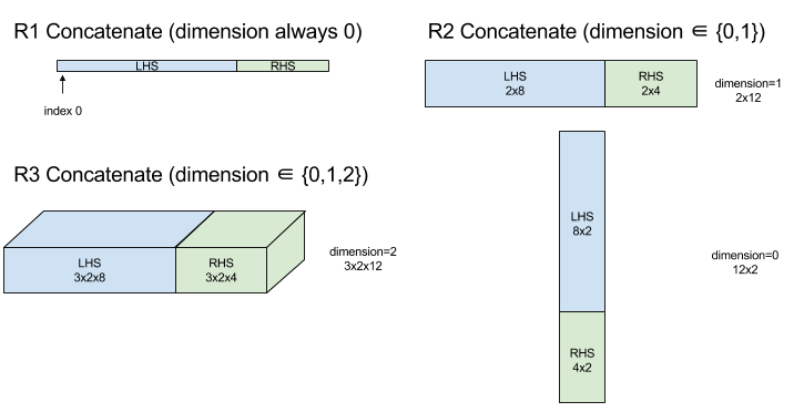
Concatenate
Consulta también XlaBuilder::ConcatInDim.
Concatenate compone un array a partir de múltiples operandos de array. El array tiene la misma clasificación que cada uno de los operandos del array de entrada (que deben ser del mismo rango) y contiene los argumentos en el orden en que se especificaron.
Concatenate(operands..., dimension)
| Argumentos | Tipo | Semántica |
|---|---|---|
operands |
secuencia de N XlaOp |
N arrays de tipo T con dimensiones [L0, L1, ...]. Requiere N >= 1. |
dimension |
int64 |
Es un valor en el intervalo [0, N) que nombra la dimensión que se concatena entre operands. |
A excepción de dimension, todas las dimensiones deben ser iguales. Esto se debe a que XLA no admite arreglos irregulares. También ten en cuenta que los valores de rango 0 no se pueden concatenar (ya que es imposible nombrar la dimensión en la que se produce la concatenación).
Ejemplo unidimensional:
Concat({ {2, 3}, {4, 5}, {6, 7} }, 0)
>>> {2, 3, 4, 5, 6, 7}
Ejemplo bidimensional:
let a = {
{1, 2},
{3, 4},
{5, 6},
};
let b = {
{7, 8},
};
Concat({a, b}, 0)
>>> {
{1, 2},
{3, 4},
{5, 6},
{7, 8},
}
Diagrama:
Condicionales
Consulta también XlaBuilder::Conditional.
Conditional(pred, true_operand, true_computation, false_operand,
false_computation)
| Argumentos | Tipo | Semántica |
|---|---|---|
pred |
XlaOp |
Escalar de tipo PRED |
true_operand |
XlaOp |
Argumento de tipo \(T_0\) |
true_computation |
XlaComputation |
XlaComputation de tipo \(T_0 \to S\) |
false_operand |
XlaOp |
Argumento de tipo \(T_1\) |
false_computation |
XlaComputation |
XlaComputation de tipo \(T_1 \to S\) |
Ejecuta true_computation si pred es true, false_computation si pred es false, y muestra el resultado.
El true_computation debe tener un solo argumento de tipo \(T_0\) y se invocará con true_operand, que debe ser del mismo tipo. false_computation debe tomar un solo argumento de tipo \(T_1\) y se invocará con false_operand, que debe ser del mismo tipo. El tipo de valor que se muestra de true_computation y false_computation debe ser el mismo.
Ten en cuenta que solo se ejecutará true_computation o false_computation según el valor de pred.
Conditional(branch_index, branch_computations, branch_operands)
| Argumentos | Tipo | Semántica |
|---|---|---|
branch_index |
XlaOp |
Escalar de tipo S32 |
branch_computations |
secuencia de N XlaComputation |
XlaComputations de tipo \(T_0 \to S , T_1 \to S , ..., T_{N-1} \to S\) |
branch_operands |
secuencia de N XlaOp |
Argumentos de tipo \(T_0 , T_1 , ..., T_{N-1}\) |
Ejecuta branch_computations[branch_index] y muestra el resultado. Si branch_index es una S32 que es < 0 o >= N, entonces branch_computations[N-1] se ejecuta como la rama predeterminada.
Cada branch_computations[b] debe recibir un solo argumento de tipo \(T_b\) y se invocará con branch_operands[b], que debe ser del mismo tipo. El tipo del valor que se muestra de cada branch_computations[b] debe ser el mismo.
Ten en cuenta que solo se ejecutará uno de los branch_computations según el valor de branch_index.
Conv. (convolución)
Consulta también XlaBuilder::Conv.
Como ConvWithGeneralPadding, pero el padding se especifica de forma abreviada como SAME o VALID. El relleno SAME rellena la entrada (lhs) con ceros para que la salida tenga la misma forma que la entrada cuando no se tiene en cuenta. Si el relleno es VÁLIDO, simplemente significa que no hay relleno.
ConvWithGeneralPadding (convolución)
Consulta también XlaBuilder::ConvWithGeneralPadding.
Calcula una convolución del tipo que se usa en las redes neuronales. Aquí, una convolución puede considerarse como una ventana de n dimensiones que se mueve a través de un área de base de n dimensiones y se realiza un cálculo para cada posición posible de la ventana.
| Argumentos | Tipo | Semántica |
|---|---|---|
lhs |
XlaOp |
rango de matriz n+2 de entradas |
rhs |
XlaOp |
Rango de n+2 de pesos de kernel |
window_strides |
ArraySlice<int64> |
Array n-d de segmentos de kernel |
padding |
ArraySlice< pair<int64,int64>> |
Array n-d de relleno (bajo, alto) |
lhs_dilation |
ArraySlice<int64> |
Matriz del factor de dilatación de n-d lhs |
rhs_dilation |
ArraySlice<int64> |
Matriz de factores de dilatación de n-d de RHS |
feature_group_count |
int64 | la cantidad de grupos de funciones |
batch_group_count |
int64 | la cantidad de grupos por lotes |
Supongamos que n es el número de dimensiones espaciales. El argumento lhs es un array de rango n+2 que describe el área de la base. Esto se llama entrada, aunque, por supuesto,
el RHS también es una entrada. En una red neuronal, estas son las activaciones de entrada.
Las dimensiones de n+2 están en este orden:
batch: Cada coordenada en esta dimensión representa una entrada independiente para la cual se realiza la convolución.z/depth/features: Cada posición (y,x) en el área base tiene un vector asociado, que entra en esta dimensión.spatial_dims: Describe las dimensiones espacialesnque definen el área base por la que se mueve la ventana.
El argumento rhs es un array de rango n+2 que describe el filtro convolucional, kernel o ventana. Las dimensiones están en este orden:
output-z: Es la dimensiónzdel resultado.input-z: El tamaño de esta dimensión porfeature_group_countdebe ser igual al tamaño de la dimensiónzen lh.spatial_dims: Describe las dimensiones espacialesnque definen la ventana n-d que se mueve por el área de la base.
El argumento window_strides especifica el segmento de la ventana convolucional en las dimensiones espaciales. Por ejemplo, si el segmento de la primera dimensión espacial es 3, la ventana solo se puede colocar en las coordenadas donde el primer índice espacial es divisible por 3.
El argumento padding especifica la cantidad de padding cero que se aplicará al área de la base. La cantidad de padding puede ser negativa: el valor absoluto del padding negativo indica la cantidad de elementos que se deben quitar de la dimensión especificada antes de hacer la convolución. padding[0] especifica el padding para la dimensión y y padding[1] especifica el padding para la dimensión x. Cada par tiene el padding bajo como primer elemento y el alto padding como el segundo elemento. El padding bajo se aplica en la dirección de los índices más bajos, mientras que el padding alto se aplica en la dirección de los índices más altos. Por ejemplo, si padding[1] es (2,3), habrá un padding de 2 ceros a la izquierda y de 3 ceros a la derecha en la segunda dimensión espacial. El uso de padding es equivalente a insertar esos mismos valores de cero en la entrada (lhs) antes de realizar la convolución.
Los argumentos lhs_dilation y rhs_dilation especifican el factor de dilatación que se aplicará a las lh y rhs, respectivamente, en cada dimensión espacial. Si el factor de dilatación en una dimensión espacial es d, los agujeros d-1 se colocan implícitamente entre cada una de las entradas de esa dimensión, lo que aumenta el tamaño del arreglo. Los agujeros se llenan con un valor no-ops, que para la convolución significa ceros.
La dilatación del rhs también se conoce como convolución atros. Para obtener más información, consulta tf.nn.atrous_conv2d. La dilatación de las lhs también se denomina convolución transpuesta. Para obtener más información, consulta tf.nn.conv2d_transpose.
El argumento feature_group_count (valor predeterminado 1) se puede usar para las convoluciones agrupadas. feature_group_count debe ser un divisor de la dimensión del atributo de entrada y de la salida. Si feature_group_count es mayor que 1, significa que, conceptualmente, la dimensión del atributo de entrada y salida y la dimensión del atributo de salida rhs se dividen de manera uniforme en muchos grupos de feature_group_count, cada uno de los cuales consta de una subsecuencia consecutiva de atributos. La dimensión del atributo de entrada de rhs debe ser igual a la dimensión del atributo de entrada lhs dividida por feature_group_count (por lo que ya tiene el tamaño de un grupo de atributos de entrada). Los grupos i-th se usan juntos a fin de calcular feature_group_count para muchas convoluciones diferentes. Los resultados de estas convoluciones se concatenan juntos en la dimensión del atributo de salida.
Para la convolución a nivel de profundidad, el argumento feature_group_count se establecería en la dimensión del atributo de entrada y el filtro se cambiaría de [filter_height, filter_width, in_channels, channel_multiplier] a [filter_height, filter_width, 1, in_channels * channel_multiplier]. Para obtener más información, consulta tf.nn.depthwise_conv2d.
El argumento batch_group_count (valor predeterminado 1) se puede usar para los filtros agrupados durante la propagación inversa. batch_group_count debe ser un divisor del tamaño de la dimensión del lote lhs (entrada). Si batch_group_count es mayor que 1, significa que la dimensión del lote de salida debe tener el tamaño input batch
/ batch_group_count. El batch_group_count debe ser un divisor del tamaño del atributo de salida.
La forma de salida tiene estas dimensiones, en este orden:
batch: El tamaño de esta dimensión porbatch_group_countdebe ser igual al tamaño de la dimensiónbatchen lh.z: Tiene el mismo tamaño queoutput-zen el kernel (rhs).spatial_dims: Un valor para cada posición válida de la ventana convolucional.

En la figura anterior, se muestra cómo funciona el campo batch_group_count. De hecho, dividimos cada lote de LH en grupos batch_group_count y hacemos lo mismo con las funciones de salida. Luego, para cada uno de estos grupos, realizamos convoluciones en pares y concatenamos la salida junto con la dimensión del atributo de salida. La semántica operativa de todas las demás dimensiones (característica y espacial) sigue siendo la misma.
Las posiciones válidas de la ventana convolucional se determinan por las zancadas y el tamaño del área de la base después del relleno.
Para describir lo que hace una convolución, considera una convolución en 2d y elige algunas coordenadas fijas batch, z, y y x en el resultado. Por lo tanto, (y,x) es la posición de una esquina de la ventana dentro del área de la base (p.ej., la esquina superior izquierda, según cómo interpretes las dimensiones espaciales). Ahora tenemos una ventana de 2D, tomada del área de la base, en la que cada punto 2d está asociado a un vector 1d, por lo que obtenemos un cuadro 3d. Desde el kernel convolucional, ya que corregimos la coordenada de salida z, también tenemos un cuadro 3D. Los dos cuadros tienen las mismas dimensiones, por lo que podemos tomar la suma de los productos a nivel de elementos entre los dos cuadros (similar a un producto escalar). Ese es el valor de salida.
Ten en cuenta que si output-z es p.ej., 5, cada posición de la ventana produce 5 valores en el resultado en la dimensión z del resultado. Estos valores difieren en qué parte del kernel convolucional se usa. Hay una caja 3D independiente de valores que se usa para cada coordenada output-z. Puedes pensar en 5 convoluciones separadas
con un filtro diferente para cada una.
A continuación, se muestra el pseudocódigo de una convolución 2d con relleno y zancadas:
for (b, oz, oy, ox) {  // output coordinates
  value = 0;
  for (iz, ky, kx) {  // kernel coordinates and input z
    iy = oy*stride_y + ky - pad_low_y;
    ix = ox*stride_x + kx - pad_low_x;
    if ((iy, ix) inside the base area considered without padding) {
      value += input(b, iz, iy, ix) * kernel(oz, iz, ky, kx);
    }
  }
  output(b, oz, oy, ox) = value;
}
ConvertElementType
Consulta también XlaBuilder::ConvertElementType.
De manera similar a un static_cast a nivel de elementos en C++, realiza una operación de conversión a nivel de elementos desde una forma de datos hasta una forma objetivo. Las dimensiones deben coincidir y la conversión se realiza en función de los elementos; p.ej., los elementos s32 se convierten en elementos f32 mediante una rutina de conversión de s32 a f32.
ConvertElementType(operand, new_element_type)
| Argumentos | Tipo | Semántica |
|---|---|---|
operand |
XlaOp |
matriz de tipo T con atenuaciones D |
new_element_type |
PrimitiveType |
tipo U |
Las dimensiones del operando y la forma objetivo deben coincidir. Los tipos de elementos de origen y destino no deben ser tuplas.
Una conversión, como de T=s32 a U=f32, realizará una rutina de conversión de valor entero a flotante normalizado, como el redondeo a par más cercano.
let a: s32[3] = {0, 1, 2};
let b: f32[3] = convert(a, f32);
then b == f32[3]{0.0, 1.0, 2.0}
CrossReplicaSum
Realiza AllReduce con un cálculo de suma.
CustomCall
Consulta también XlaBuilder::CustomCall.
Llama a una función proporcionada por el usuario dentro de un cálculo.
CustomCall(target_name, args..., shape)
| Argumentos | Tipo | Semántica |
|---|---|---|
target_name |
string |
Nombre de la función. Se emitirá una instrucción de llamada orientada a este nombre de símbolo. |
args |
secuencia de N XlaOp |
N argumentos de tipo arbitrario, que se pasarán a la función. |
shape |
Shape |
Forma del resultado de la función |
La firma de la función es la misma, sin importar la arquitectura o el tipo de argumentos:
extern "C" void target_name(void* out, void** in);
Por ejemplo, si CustomCall se usa de la siguiente manera:
let x = f32[2] {1,2};
let y = f32[2x3] { {10, 20, 30}, {40, 50, 60} };

CustomCall("myfunc", {x, y}, f32[3x3])
A continuación, se muestra un ejemplo de una implementación de myfunc:
extern "C" void myfunc(void* out, void** in) {
  float (&x)[2] = *static_cast<float(*)[2]>(in[0]);
  float (&y)[2][3] = *static_cast<float(*)[2][3]>(in[1]);
  EXPECT_EQ(1, x[0]);
  EXPECT_EQ(2, x[1]);
  EXPECT_EQ(10, y[0][0]);
  EXPECT_EQ(20, y[0][1]);
  EXPECT_EQ(30, y[0][2]);
  EXPECT_EQ(40, y[1][0]);
  EXPECT_EQ(50, y[1][1]);
  EXPECT_EQ(60, y[1][2]);
  float (&z)[3][3] = *static_cast<float(*)[3][3]>(out);
  z[0][0] = x[1] + y[1][0];
  // ...
}
La función proporcionada por el usuario no debe tener efectos secundarios y su ejecución debe ser idempotente.
Punto
Consulta también XlaBuilder::Dot.
Dot(lhs, rhs)
| Argumentos | Tipo | Semántica |
|---|---|---|
lhs |
XlaOp |
array de tipo T |
rhs |
XlaOp |
array de tipo T |
La semántica exacta de esta operación depende de las clasificaciones de los operandos:
| Entrada | Resultado | Semántica |
|---|---|---|
vector [n] dot vector [n] |
escalar | producto escalar vectorial |
matriz [m x k] vector dot [k] |
vector [m] | multiplicación de vectores y matrices |
matriz [m x k] dot matriz [k x n] |
matriz [m x n] | multiplicación de matrices-matriz |
La operación realiza la suma de los productos en la segunda dimensión de lhs (o
el primero si tiene clasificación 1) y la primera dimensión de rhs. Estas son las dimensiones "contratadas". Las dimensiones contraídas de lhs y rhs deben ser del mismo tamaño. En la práctica, se puede usar para realizar productos escalares entre vectores, multiplicaciones de vectores y matrices o multiplicaciones de matrices y matrices.
DotGeneral
Consulta también XlaBuilder::DotGeneral.
DotGeneral(lhs, rhs, dimension_numbers)
| Argumentos | Tipo | Semántica |
|---|---|---|
lhs |
XlaOp |
array de tipo T |
rhs |
XlaOp |
array de tipo T |
dimension_numbers |
DotDimensionNumbers |
números de dimensión de lotes y de contratación |
Es similar a Dot, pero permite que se especifiquen los números de la dimensión del lote y de la contratación para lhs y rhs.
| Campos DotDimensionNumbers | Tipo | Semántica |
|---|---|---|
lhs_contracting_dimensions
|
int64 repetido | lhs números de dimensión de contrato |
rhs_contracting_dimensions
|
int64 repetido | rhs números de dimensión de contrato |
lhs_batch_dimensions
|
int64 repetido | lhs de números de dimensiones del lote |
rhs_batch_dimensions
|
int64 repetido | rhs de números de dimensiones del lote |
DotGeneral realiza la suma de productos sobre las dimensiones de contratación especificadas en dimension_numbers.
No es necesario que los números de dimensión de contratación asociados de lhs y rhs sean los mismos, pero deben tener los mismos tamaños de dimensión.
Ejemplo con números de dimensión contratados:
lhs = { {1.0, 2.0, 3.0},
{4.0, 5.0, 6.0} }

rhs = { {1.0, 1.0, 1.0},
{2.0, 2.0, 2.0} }

DotDimensionNumbers dnums;
dnums.add_lhs_contracting_dimensions(1);
dnums.add_rhs_contracting_dimensions(1);

DotGeneral(lhs, rhs, dnums) -> { {6.0, 12.0},
{15.0, 30.0} }
Los números de dimensión del lote asociados de lhs y rhs deben tener los mismos tamaños de dimensión.
Ejemplo con números de dimensiones del lote (tamaño del lote 2, matrices de 2 x 2):
lhs = { { {1.0, 2.0},
{3.0, 4.0} },
{ {5.0, 6.0},
{7.0, 8.0} } }

rhs = { { {1.0, 0.0},
{0.0, 1.0} },
{ {1.0, 0.0},
{0.0, 1.0} } }

DotDimensionNumbers dnums;
dnums.add_lhs_contracting_dimensions(2);
dnums.add_rhs_contracting_dimensions(1);
dnums.add_lhs_batch_dimensions(0);
dnums.add_rhs_batch_dimensions(0);

DotGeneral(lhs, rhs, dnums) -> { { {1.0, 2.0},
{3.0, 4.0} },
{ {5.0, 6.0},
{7.0, 8.0} } }
| Entrada | Resultado | Semántica |
|---|---|---|
[b0, m, k] dot [b0, k, n] |
[b0, m, n]. | matmul por lotes |
[b0, b1, m, k] dot [b0, b1, k, n] |
[b0, b1, m, n]. | matmul por lotes |
Luego, el número de dimensión resultante comienza con la dimensión del lote, luego con la dimensión no contractual o no por lotes de lhs y, por último, la dimensión rhs no contratada o no por lotes.
DynamicSlice
Consulta también XlaBuilder::DynamicSlice.
DynamicSlice extrae un subarreglo del arreglo de entrada en start_indices dinámico. El tamaño de la porción en cada dimensión se pasa en size_indices, que especifica el punto de finalización de los intervalos de porción exclusivos en cada dimensión: [inicio, inicio + tamaño). La forma de start_indices debe tener una clasificación == 1, con un tamaño de dimensión igual al rango de operand.
DynamicSlice(operand, start_indices, size_indices)
| Argumentos | Tipo | Semántica |
|---|---|---|
operand |
XlaOp |
Arreglo n-dimensional de tipo T |
start_indices |
secuencia de N XlaOp |
Lista de N números enteros escalares que contienen los índices iniciales de la porción para cada dimensión. El valor debe ser mayor o igual que cero. |
size_indices |
ArraySlice<int64> |
Lista de N números enteros que contienen el tamaño de la porción para cada dimensión. Cada valor debe ser estrictamente mayor que cero, y el valor de inicio + tamaño debe ser menor o igual que el tamaño de la dimensión para evitar ajustar el tamaño de la dimensión de módulo. |
Los índices de porción efectivos se calculan mediante la aplicación de la siguiente transformación para cada índice i en [1, N) antes de realizar la porción:
start_indices[i] = clamp(start_indices[i], 0, operand.dimension_size[i] - size_indices[i])
Esto garantiza que la porción extraída siempre esté dentro de los límites del arreglo de operando. Si la porción está dentro de los límites antes de que se aplique la transformación, esta no tiene efecto.
Ejemplo unidimensional:
let a = {0.0, 1.0, 2.0, 3.0, 4.0}
let s = {2}

DynamicSlice(a, s, {2}) produces:
{2.0, 3.0}
Ejemplo bidimensional:
let b =
{ {0.0,  1.0,  2.0},
{3.0,  4.0,  5.0},
{6.0,  7.0,  8.0},
{9.0, 10.0, 11.0} }
let s = {2, 1}

DynamicSlice(b, s, {2, 2}) produces:
{ { 7.0,  8.0},
{10.0, 11.0} }
DynamicUpdateSlice
Consulta también XlaBuilder::DynamicUpdateSlice.
DynamicUpdateSlice genera un resultado que es el valor del arreglo de entrada operand, con una porción update reemplazada en start_indices.
La forma de update determina la forma del subarray del resultado que se actualiza.
La forma de start_indices debe tener una clasificación == 1, con un tamaño de dimensión igual al rango de operand.
DynamicUpdateSlice(operand, update, start_indices)
| Argumentos | Tipo | Semántica |
|---|---|---|
operand |
XlaOp |
Arreglo n-dimensional de tipo T |
update |
XlaOp |
Arreglo n dimensional de tipo T que contiene la actualización de la porción. Cada dimensión de la forma de actualización debe ser estrictamente mayor que cero, y el valor de inicio + actualización debe ser menor o igual que el tamaño del operando de cada dimensión para evitar que se generen índices de actualización fuera de los límites. |
start_indices |
secuencia de N XlaOp |
Lista de N números enteros escalares que contienen los índices iniciales de la porción para cada dimensión. El valor debe ser mayor o igual que cero. |
Los índices de porción efectivos se calculan mediante la aplicación de la siguiente transformación para cada índice i en [1, N) antes de realizar la porción:
start_indices[i] = clamp(start_indices[i], 0, operand.dimension_size[i] - update.dimension_size[i])
Esto garantiza que la porción actualizada esté siempre dentro de los límites del arreglo de operando. Si la porción está dentro de los límites antes de que se aplique la transformación, esta no tiene efecto.
Ejemplo unidimensional:
let a = {0.0, 1.0, 2.0, 3.0, 4.0}
let u = {5.0, 6.0}
let s = {2}

DynamicUpdateSlice(a, u, s) produces:
{0.0, 1.0, 5.0, 6.0, 4.0}
Ejemplo bidimensional:
let b =
{ {0.0,  1.0,  2.0},
{3.0,  4.0,  5.0},
{6.0,  7.0,  8.0},
{9.0, 10.0, 11.0} }
let u =
{ {12.0,  13.0},
{14.0,  15.0},
{16.0,  17.0} }

let s = {1, 1}

DynamicUpdateSlice(b, u, s) produces:
{ {0.0,  1.0,  2.0},
{3.0, 12.0, 13.0},
{6.0, 14.0, 15.0},
{9.0, 16.0, 17.0} }
Operaciones aritméticas binarias en elementos
Consulta también XlaBuilder::Add.
Se admite un conjunto de operaciones aritméticas binarias a nivel de elementos.
Op(lhs, rhs)
Donde Op es uno de Add (suma), Sub (resta), Mul (multiplicación), Div (división), Rem (resto), Max (máximo), Min (mínimo), LogicalAnd (operación lógica AND) o LogicalOr (operación lógica OR).
| Argumentos | Tipo | Semántica |
|---|---|---|
lhs |
XlaOp |
operando izquierdo: matriz de tipo T |
rhs |
XlaOp |
operando derecho: array de tipo T |
Las formas de los argumentos deben ser similares o compatibles. Consulta la documentación de transmisión sobre lo que significa que las formas sean compatibles. El resultado de una operación tiene una forma que es el resultado de transmitir los dos arreglos de entrada. En esta variante, las operaciones entre arreglos de diferentes rangos no son compatibles, a menos que uno de los operandos sea un escalar.
Cuando Op es Rem, el signo del resultado se toma del dividendo, y el valor absoluto del resultado siempre es menor que el valor absoluto del divisor.
El desbordamiento de división de enteros (división/resto con firma o sin firma por cero o división o resto con firma de INT_SMIN con -1) produce un valor definido de implementación.
Existe una variante alternativa compatible con la transmisión de diferentes rangos para estas operaciones:
Op(lhs, rhs, broadcast_dimensions)
En el ejemplo anterior, Op es igual al anterior. Esta variante de la operación debe usarse para operaciones aritméticas entre arreglos de diferentes rangos (por ejemplo, agregar una matriz a un vector).
El operando broadcast_dimensions adicional es una porción de números enteros que se usa para expandir el rango del operando de rango inferior hasta el rango del operando de rango superior. broadcast_dimensions asigna las dimensiones de la forma de rango inferior a las dimensiones de la forma de rango superior. Las dimensiones sin asignar de la forma expandida se rellenan con dimensiones de tamaño uno. Luego, la transmisión de la degeneración de dimensión transmite las formas a lo largo de estas dimensiones degeneradas para igualar las formas de ambos operandos. La semántica se describe en detalle en la página de transmisión.
Operaciones de comparación en elementos
Consulta también XlaBuilder::Eq.
Se admite un conjunto de operaciones de comparación binaria estándar por elementos. Ten en cuenta que se aplica la semántica de comparación de punto flotante estándar IEEE 754 cuando se comparan tipos de punto flotante.
Op(lhs, rhs)
Donde Op es uno de Eq (igual a), Ne (no igual a), Ge (mayor o igual que), Gt (mayor que), Le (menor o igual que), Lt (menor que). Otro conjunto de operadores, EqTotalOrder, NeTotalOrder, GeTotalOrder, GtTotalOrder, LeTotalOrder y LtTotalOrder, proporcionan las mismas funcionalidades, excepto que, además, admiten un pedido total sobre los números de punto flotante. Para ello, aplican -NaN < -Inf < -Finite < -0 < +0 < +NFinite < +N.
| Argumentos | Tipo | Semántica |
|---|---|---|
lhs |
XlaOp |
operando izquierdo: matriz de tipo T |
rhs |
XlaOp |
operando derecho: array de tipo T |
Las formas de los argumentos deben ser similares o compatibles. Consulta la documentación de transmisión sobre lo que significa que las formas sean compatibles. El resultado de una operación tiene una forma que es el resultado de transmitir los dos arrays de entrada con el tipo de elemento PRED. En esta variante, no se admiten las operaciones entre arreglos de diferentes rangos, a menos que uno de los operandos sea un escalar.
Existe una variante alternativa compatible con la transmisión de diferentes rangos para estas operaciones:
Op(lhs, rhs, broadcast_dimensions)
En el ejemplo anterior, Op es igual al anterior. Esta variante de la operación se debe usar para operaciones de comparación entre arreglos de diferentes rangos (por ejemplo, agregar una matriz a un vector).
El operando broadcast_dimensions adicional es una porción de números enteros que especifican las dimensiones que se usarán para transmitir los operandos. La semántica se describe en detalle en la página de transmisión.
Funciones unarias en elementos
XlaBuilder admite estas funciones unarias a nivel de elementos:
Abs(operand) Abs. a nivel de los elementos x -> |x|.
Ceil(operand) Ceil de elementos x -> ⌈x⌉.
Cos(operand) Coseno del elemento x -> cos(x).
Exp(operand) exponencial natural de elementos x -> e^x.
Floor(operand) Base del elemento x -> ⌊x⌋.
Imag(operand) Parte imaginaria con elementos de una forma compleja (o real). x -> imag(x). Si el operando es un tipo de punto flotante, muestra 0.
IsFinite(operand): Comprueba si cada elemento de operand es finito, es decir, no es infinito positivo o negativo y no es NaN. Muestra un array de valores PRED con la misma forma que la entrada, en el que cada elemento es true solo si el elemento de entrada correspondiente es finito.
Log(operand) Logaritmo natural de los elementos x -> ln(x).
LogicalNot(operand) Lógico a nivel de elemento, no x -> !(x).
Logistic(operand) Cálculo de la función logística por elementos x ->
logistic(x).
PopulationCount(operand): Calcula la cantidad de bits configurados en cada elemento de operand.
Neg(operand) Negación a nivel del elemento x -> -x.
Real(operand) Parte real con elementos de una forma compleja (o real).
x -> real(x). Si el operando es un tipo de punto flotante, muestra el mismo valor.
Rsqrt(operand) Recíproco a nivel de elemento de la operación de raíz cuadrada x -> 1.0 / sqrt(x).
Sign(operand) Operación de signo a nivel del elemento x -> sgn(x) donde
\[\text{sgn}(x) = \begin{cases} -1 & x < 0\\ -0 & x = -0\\ NaN & x = NaN\\ +0 & x = +0\\ 1 & x > 0 \end{cases}\]
Mediante el operador de comparación del tipo de elemento de operand.
Sqrt(operand) Operación de raíz cuadrada por elementos x -> sqrt(x).
Cbrt(operand) Operación de raíz cúbica a nivel del elemento x -> cbrt(x).
Tanh(operand) Tangente hiperbólica por elementos x -> tanh(x).
Round(operand) Redondeo a nivel de los elementos, empatado de cero.
RoundNearestEven(operand) Redondeo por elementos, se vincula al par más cercano.
| Argumentos | Tipo | Semántica |
|---|---|---|
operand |
XlaOp |
El operando para la función |
La función se aplica a cada elemento del array operand, lo que da como resultado un array con la misma forma. Se permite que operand sea un escalar (rango 0).
Fft
La operación FFT de XLA implementa las transformadas de Fourier inversas y directas para entradas y salidas reales y complejas. Se admiten los FFT multidimensionales en hasta 3 ejes.
Consulta también XlaBuilder::Fft.
| Argumentos | Tipo | Semántica |
|---|---|---|
operand |
XlaOp |
La matriz que estamos transformando Fourier. |
fft_type |
FftType |
Consulta la tabla que se encuentra a continuación |
fft_length |
ArraySlice<int64> |
Las longitudes en dominios del tiempo de los ejes que se transforman. Esto es necesario en particular para que IRFFT ajuste el tamaño del eje más interno, ya que RFFT(fft_length=[16]) tiene la misma forma de salida que RFFT(fft_length=[17]). |
FftType |
Semántica |
|---|---|
FFT |
Reenviar FFT de complejo a complejo. La forma no se modificó. |
IFFT |
FFT de complejo a complejo inverso. La forma no se modificó. |
RFFT |
Reenviar FFT reales a complejos. La forma del eje más interno se reduce a fft_length[-1] // 2 + 1 si fft_length[-1] es un valor distinto de cero y se omite la parte conjugada invertida de la señal transformada más allá de la frecuencia de Nyquist. |
IRFFT |
FFT inverso de real a complejo (es decir, toma complejo, muestra real) La forma del eje más interno se expande a fft_length[-1] si fft_length[-1] es un valor distinto de cero, lo que infiere la parte de la señal transformada más allá de la frecuencia de Nyquist desde el conjugado inverso de las entradas 1 a fft_length[-1] // 2 + 1. |
FFT multidimensional
Cuando se proporciona más de 1 fft_length, esto equivale a aplicar una cascada de operaciones FFT a cada uno de los ejes más internos. Ten en cuenta que, en los casos reales->complejos y complejos-> reales, la transformación del eje más interno se realiza (de forma efectiva) primero (RFFT; último para IRFFT), por lo que el eje más interno es el que cambia de tamaño. Otras transformaciones de ejes serán
complejas > complejas.
Detalles de la implementación
El FFT de la CPU está respaldado por el TensorFFT de Eigen. La FFT de la GPU usa cuFFT.
Gather
La operación de recopilación de XLA une varias porciones (cada una en un desplazamiento de tiempo de ejecución potencialmente diferente) de un array de entrada.
Semántica general
Consulta también XlaBuilder::Gather.
Para obtener una descripción más intuitiva, consulta la sección "Descripción informal" a continuación.
gather(operand, start_indices, offset_dims, collapsed_slice_dims, slice_sizes, start_index_map)
| Argumentos | Tipo | Semántica |
|---|---|---|
operand |
XlaOp |
El array del que estamos recopilando. |
start_indices |
XlaOp |
Arreglo que contiene los índices iniciales de las porciones que recopilamos. |
index_vector_dim |
int64 |
Es la dimensión de start_indices que "contiene" los índices iniciales. Consulta la siguiente información para obtener una descripción detallada. |
offset_dims |
ArraySlice<int64> |
El conjunto de dimensiones en la forma de salida que se desplazan en un arreglo dividido del operando. |
slice_sizes |
ArraySlice<int64> |
slice_sizes[i] son los límites de la porción en la dimensión i. |
collapsed_slice_dims |
ArraySlice<int64> |
El conjunto de dimensiones en cada porción que se contraen. Estas dimensiones deben tener un tamaño de 1. |
start_index_map |
ArraySlice<int64> |
Mapa en el que se describe cómo asignar los índices de start_indices a los índices legales en un operando. |
indices_are_sorted |
bool |
Indica si se garantiza que los índices estén ordenados por el emisor. |
unique_indices |
bool |
Indica si el emisor garantiza que los índices sean únicos. |
Para mayor comodidad, etiquetamos las dimensiones en el array de salida no en offset_dims como batch_dims.
El resultado es un array de clasificación batch_dims.size + offset_dims.size.
operand.rank debe ser igual a la suma de offset_dims.size y collapsed_slice_dims.size. Además, slice_sizes.size debe ser igual a operand.rank.
Si index_vector_dim es igual a start_indices.rank, consideramos implícitamente que start_indices tiene una dimensión 1 final (es decir, si start_indices tenía la forma [6,7] y index_vector_dim es 2, consideramos implícitamente que la forma de start_indices es [6,7,1]).
Los límites del array de salida junto con la dimensión i se calculan de la siguiente manera:
Si
iestá presente enbatch_dims(es decir, es igual abatch_dims[k]para algunosk), elegimos los límites de dimensión correspondientes destart_indices.shapey se omiteindex_vector_dim(es decir, seleccionastart_indices.shape.dims[k] sik<index_vector_dimystart_indices.shape.dims[k+1] de lo contrario).Si
iestá presente enoffset_dims(es decir, igual aoffset_dims[k] para algunosk), elegimos el límite correspondiente deslice_sizesdespués de considerarcollapsed_slice_dims(es decir, seleccionamosadjusted_slice_sizes[k], en el queadjusted_slice_sizesesslice_sizescon los límites de los índicescollapsed_slice_dimsquitados).
De manera formal, el índice de operando In correspondiente a un índice de salida determinado Out se calcula de la siguiente manera:
Supongamos que
G= {Out[k] parakenbatch_dims}. UsaGpara dividir un vectorSde modo queS[i] =start_indices[Combine(G,i)], en el que Combine(A, b) inserta b en la posiciónindex_vector_dimen A. Ten en cuenta que esto está bien definido, incluso siGestá vacío: siGestá vacío, entoncesS=start_indices.Crea un índice inicial,
Sin, enoperandmedianteSmediante la dispersión deSmediantestart_index_map. Para ser más precisos:Sin[start_index_map[k]] =S[k] sik<start_index_map.size.Sin[_] =0de lo contrario.
Crea un índice
Oinenoperandmediante la dispersión de los índices en las dimensiones de desplazamiento enOutde acuerdo con el conjunto decollapsed_slice_dims. Para ser más precisos:Oin[remapped_offset_dims(k)] =Out[offset_dims[k]] sik<offset_dims.size(remapped_offset_dimsse define a continuación).Oin[_] =0de lo contrario.
InesOin+Sin, donde + representa la suma a nivel de los elementos.
remapped_offset_dims es una función monótona con dominio [0, offset_dims.size) y rango [0, operand.rank) \ collapsed_slice_dims. Entonces,
si, p.ej., offset_dims.size es 4, operand.rank es 6 y collapsed_slice_dims es {0, 2}, luego, remapped_offset_dims es {0→1, 1→3, 2→4, 3→5}.
Si se configura indices_are_sorted como verdadero, XLA puede suponer que el usuario ordena start_indices (en orden ascendente start_index_map). Si no lo son, la implementación se define en la semántica.
Si unique_indices se establece como verdadero, XLA puede suponer que todos los elementos dispersos son únicos. Por lo tanto, XLA podría usar operaciones no atómicas. Si unique_indices se establece como verdadero y los índices dispersos no son únicos, la implementación se define en la semántica.
Descripción informal y ejemplos
Informalmente, cada índice Out del array de salida corresponde a un elemento E en el array de operando, lo que se calcula de la siguiente manera:
Usamos las dimensiones del lote en
Outpara buscar un índice de inicio a partir destart_indices.Usamos
start_index_mappara asignar el índice inicial (cuyo tamaño puede ser menor que operand.rank) a un índice inicial "completo" enoperand.Dividimos de forma dinámica una porción con el tamaño
slice_sizesusando el índice de inicio completo.Para cambiar la forma de la porción, contraemos las dimensiones de
collapsed_slice_dims. Dado que todas las dimensiones de segmentos contraídos deben tener un límite de 1, este cambio de forma siempre es legal.Usamos las dimensiones de desplazamiento en
Outpara indexar en esta porción y obtener el elemento de entrada,E, que corresponde al índice de salidaOut.
index_vector_dim se configura como start_indices.rank: 1 en todos los ejemplos que siguen. Los valores más interesantes de index_vector_dim no cambian la operación en esencia, pero hacen que la representación visual sea más engorrosa.
Para tener una intuición de cómo se combina todo lo anterior, veamos un ejemplo en el que se reúnen 5 porciones de forma [8,6] de un array [16,11]. La posición de una porción en el array [16,11] se puede representar como un vector de índice de la forma S64[2], por lo que el conjunto de 5 posiciones se puede representar como un array S64[5,2].
El comportamiento de la operación de recopilación se puede representar como una transformación de índices que toma [G,O0,O1], un índice en la forma de salida y lo asigna a un elemento en el array de entrada de la siguiente manera:

Primero, seleccionamos un vector (X,Y) del array de recopilación de índices con G.
El elemento en el array de salida en el índice [G,O0,O1] es el elemento del array de entrada en el índice [X+O0,Y+O1].
slice_sizes es [8,6], que decide el rango de O0 y O1, y esto, a su vez, decide los límites de la porción.
Esta operación de recopilación actúa como una porción dinámica por lotes con G como la dimensión
del lote.
Los índices de recopilación pueden ser multidimensionales. Por ejemplo, una versión más general del ejemplo anterior que use un array de "índices de recopilación" con la forma [4,5,2] traduciría índices como el siguiente:

De nuevo, esto actúa como una porción dinámica por lotes G0 y G1 como las dimensiones del lote. El tamaño de la porción sigue siendo [8,6].
La operación de recopilación en XLA generaliza la semántica informal descrita anteriormente de las siguientes maneras:
Podemos configurar qué dimensiones de la forma de salida son las de desplazamiento (dimensiones que contienen
O0yO1en el último ejemplo). Las dimensiones del lote de salida (dimensiones que contienenG0,G1en el último ejemplo) se definen como las dimensiones de salida que no son dimensiones de desplazamiento.La cantidad de dimensiones de desplazamiento de salida presentes explícitamente en la forma de salida puede ser menor que la clasificación de entrada. Estas dimensiones "faltantes", que se enumeran explícitamente como
collapsed_slice_dims, deben tener un tamaño de porción de1. Como tienen un tamaño de porción de1, el único índice válido para ellos es0y, si los omites, no se introduce ambigüedad.Es posible que la porción extraída del arreglo “Recopilar índices” (
X,Y) en el último ejemplo) tenga menos elementos que la clasificación del arreglo de entrada, y una asignación explícita determina cómo se debe expandir el índice para que tenga la misma clasificación que la entrada.
Como ejemplo final, usamos (2) y (3) para implementar tf.gather_nd:

G0 y G1 se usan para dividir un índice inicial del array de índices recolectados como de costumbre, excepto que el índice inicial tiene un solo elemento, X. Del mismo modo, solo hay un índice de desplazamiento de salida con el valor O0. Sin embargo, antes de usarse como índices en el array de entrada, estos se expanden de acuerdo con "Recopilar asignación de índices" (start_index_map en la descripción formal) y "Asignación de desplazamiento" (remapped_offset_dims en la descripción formal) a [X,0] y [0,O0], respectivamente, y sumar [X,O0]. En otras palabras, el índice de salida [G0].G0000OOGG11GatherIndicestf.gather_nd
slice_sizes para este caso es [1,11]. De forma intuitiva, esto significa que cada índice X en el arreglo de recopilación de índices elige una fila completa y el resultado es la concatenación de todas estas filas.
GetDimensionSize
Consulta también XlaBuilder::GetDimensionSize.
Muestra el tamaño de la dimensión determinada del operando. El operando debe tener forma de arreglo.
GetDimensionSize(operand, dimension)
| Argumentos | Tipo | Semántica |
|---|---|---|
operand |
XlaOp |
array de entrada de n dimensiones |
dimension |
int64 |
Un valor en el intervalo [0, n) que especifica la dimensión |
SetDimensionSize
Consulta también XlaBuilder::SetDimensionSize.
Establece el tamaño dinámico de la dimensión determinada de XlaOp. El operando debe tener forma de arreglo.
SetDimensionSize(operand, size, dimension)
| Argumentos | Tipo | Semántica |
|---|---|---|
operand |
XlaOp |
de entrada de dimensiones n. |
size |
XlaOp |
int32, que representa el tamaño dinámico del entorno de ejecución |
dimension |
int64 |
Es un valor en el intervalo [0, n) que especifica la dimensión. |
Pasa el operando como resultado, con la dimensión dinámica que realiza el seguimiento del compilador.
Las operaciones de reducción descendentes ignorarán los valores con relleno.
let v: f32[10] = f32[10]{1, 2, 3, 4, 5, 6, 7, 8, 9, 10};
let five: s32 = 5;
let six: s32 = 6;

// Setting dynamic dimension size doesn't change the upper bound of the static
// shape.
let padded_v_five: f32[10] = set_dimension_size(v, five, /*dimension=*/0);
let padded_v_six: f32[10] = set_dimension_size(v, six, /*dimension=*/0);

// sum == 1 + 2 + 3 + 4 + 5
let sum:f32[] = reduce_sum(padded_v_five);
// product == 1 * 2 * 3 * 4 * 5
let product:f32[] = reduce_product(padded_v_five);

// Changing padding size will yield different result.
// sum == 1 + 2 + 3 + 4 + 5 + 6
let sum:f32[] = reduce_sum(padded_v_six);
GetTupleElement
Consulta también XlaBuilder::GetTupleElement.
Indexa en una tupla con un valor constante de tiempo de compilación.
El valor debe ser una constante de tiempo de compilación para que la inferencia de forma pueda determinar el tipo del valor resultante.
Es similar a std::get<int N>(t) en C++. Conceptualmente:
let v: f32[10] = f32[10]{0, 1, 2, 3, 4, 5, 6, 7, 8, 9};
let s: s32 = 5;
let t: (f32[10], s32) = tuple(v, s);
let element_1: s32 = gettupleelement(t, 1);  // Inferred shape matches s32.
Consulta también tf.tuple.
Entrada
Consulta también XlaBuilder::Infeed.
Infeed(shape)
| Argumento | Tipo | Semántica |
|---|---|---|
shape |
Shape |
Forma de los datos leídos desde la interfaz de entrada. El campo de diseño de la forma debe configurarse para que coincida con el diseño de los datos enviados al dispositivo; de lo contrario, su comportamiento no está definido. |
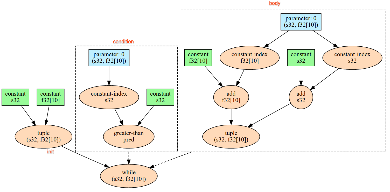
Lee un solo elemento de datos de la interfaz de transmisión de entrada implícita del dispositivo, interpreta los datos como la forma determinada y su diseño, y muestra un XlaOp de los datos. En un cálculo, se permiten varias operaciones de entrada, pero debe haber un orden total entre ellas. Por ejemplo, dos entradas del siguiente código tienen un orden total, ya que hay una dependencia entre los bucles while.
result1 = while (condition, init = init_value) {
  Infeed(shape)
}

result2 = while (condition, init = result1) {
  Infeed(shape)
}
Las formas anidadas de tuplas no son compatibles. En el caso de una forma de tupla vacía, la operación de entrada es efectivamente una no-op y continúa sin leer ningún dato de la entrada del dispositivo.
Pizca
Consulta también XlaBuilder::Iota.
Iota(shape, iota_dimension)
Compila un literal constante en el dispositivo en lugar de una transferencia de host potencialmente grande. Crea un array con una forma especificada y contiene valores que comienzan en cero y que se incrementan en uno a lo largo de la dimensión especificada. Para los tipos de punto flotante, el array producido es equivalente a ConvertElementType(Iota(...)), en el que Iota es de tipo integral y la conversión es al tipo de punto flotante.
| Argumentos | Tipo | Semántica |
|---|---|---|
shape |
Shape |
Forma del array que creó Iota() |
iota_dimension |
int64 |
La dimensión que se va a aumentar. |
Por ejemplo, Iota(s32[4, 8], 0) muestra
  [[0, 0, 0, 0, 0, 0, 0, 0 ],
   [1, 1, 1, 1, 1, 1, 1, 1 ],
   [2, 2, 2, 2, 2, 2, 2, 2 ],
   [3, 3, 3, 3, 3, 3, 3, 3 ]]
Devoluciones por Iota(s32[4, 8], 1)
  [[0, 1, 2, 3, 4, 5, 6, 7 ],
   [0, 1, 2, 3, 4, 5, 6, 7 ],
   [0, 1, 2, 3, 4, 5, 6, 7 ],
   [0, 1, 2, 3, 4, 5, 6, 7 ]]
Mapa
Consulta también XlaBuilder::Map.
Map(operands..., computation)
| Argumentos | Tipo | Semántica |
|---|---|---|
operands |
secuencia de N XlaOp |
N arrays de tipos T0..T{N-1} |
computation |
XlaComputation |
Cálculo de tipo T_0, T_1, .., T_{N + M -1} -> S con N parámetros de tipo T y M de tipo arbitrario |
dimensions |
Array de int64 |
array de dimensiones del mapa |
Aplica una función escalar sobre los arreglos operands dados, lo que produce un arreglo de las mismas dimensiones en el que cada elemento es el resultado de la función asignada aplicada a los elementos correspondientes en los arreglos de entrada.
La función asignada es un cálculo arbitrario con la restricción de que tiene N entradas del tipo escalar T y un solo resultado con el tipo S. El resultado tiene las mismas dimensiones que los operandos, excepto que el tipo de elemento T se reemplaza por S.
Por ejemplo: Map(op1, op2, op3, computation, par1) asigna elem_out <-
computation(elem1, elem2, elem3, par1) a cada índice (multidimensional) en los arrays de entrada para producir el array de salida.
OptimizationBarrier
Bloquea cualquier pase de optimización para que no desplace los cálculos por la barrera.
Garantiza que todas las entradas se evalúen antes que los operadores que dependen de las salidas de la barrera.
Almohadilla
Consulta también XlaBuilder::Pad.
Pad(operand, padding_value, padding_config)
| Argumentos | Tipo | Semántica |
|---|---|---|
operand |
XlaOp |
array de tipo T |
padding_value |
XlaOp |
escalar de tipo T para completar el padding agregado |
padding_config |
PaddingConfig |
cantidad de padding en ambos bordes (bajo, alto) y entre los elementos de cada dimensión |
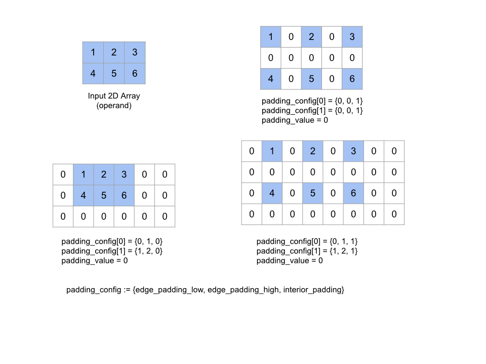
Expande el array operand dado mediante el padding alrededor del array y entre sus elementos con el padding_value especificado. padding_config especifica la cantidad de padding en el borde y el padding interior de cada dimensión.
PaddingConfig es un campo repetido de PaddingConfigDimension, que contiene tres campos para cada dimensión: edge_padding_low, edge_padding_high y interior_padding.
edge_padding_low y edge_padding_high especifican la cantidad de padding agregado en el extremo inferior (junto al índice 0) y en el extremo alto (junto al índice más alto) de cada dimensión, respectivamente. La cantidad de padding del borde puede ser negativa: el valor absoluto del padding negativo indica la cantidad de elementos que se deben quitar de la dimensión especificada.
interior_padding especifica la cantidad de padding agregado entre dos elementos cualesquiera en cada dimensión. Este valor no puede ser negativo. El padding interno se produce de manera lógica antes del padding del borde, por lo que, en el caso de un padding de borde negativo, los elementos se quitan del operando con padding interno.
Esta operación es una no-op si todos los pares de padding de bordes son (0, 0) y los valores de padding interno son todos 0. En la siguiente figura, se muestran ejemplos de diferentes valores edge_padding y interior_padding para un array bidimensional.
Recv
Consulta también XlaBuilder::Recv.
Recv(shape, channel_handle)
| Argumentos | Tipo | Semántica |
|---|---|---|
shape |
Shape |
forma de los datos para recibir |
channel_handle |
ChannelHandle |
identificador único para cada par de envío y recepción |
Recibe datos de la forma determinada desde una instrucción Send en otro cálculo que comparte el mismo controlador de canal. Muestra un XlaOp para los datos recibidos.
La API del cliente de la operación Recv representa la comunicación síncrona.
Sin embargo, la instrucción se divide internamente en 2 instrucciones HLO (Recv y RecvDone) para habilitar las transferencias de datos asíncronas. Consulta también HloInstruction::CreateRecv y HloInstruction::CreateRecvDone.
Recv(const Shape& shape, int64 channel_id)
Asigna los recursos necesarios para recibir datos de una instrucción Send con el mismo channel_id. Muestra un contexto para los recursos asignados, que se usa con la siguiente instrucción RecvDone para esperar que se complete la transferencia de datos. El contexto es una tupla de {puerto de recepción (forma), identificador de solicitud (U32)} y solo lo puede usar una instrucción RecvDone.
RecvDone(HloInstruction context)
Dado un contexto creado por una instrucción Recv, espera a que se complete la transferencia de datos y muestra los datos recibidos.
Reducir
Consulta también XlaBuilder::Reduce.
Aplica una función de reducción a uno o más arreglos en paralelo.
Reduce(operands..., init_values..., computation, dimensions)
| Argumentos | Tipo | Semántica |
|---|---|---|
operands |
Secuencia de N XlaOp |
N arrays de tipos T_0, ..., T_{N-1}. |
init_values |
Secuencia de N XlaOp |
N escalares de tipos T_0, ..., T_{N-1}. |
computation |
XlaComputation |
el cálculo de tipo T_0, ..., T_{N-1}, T_0, ..., T_{N-1} -> Collate(T_0, ..., T_{N-1}). |
dimensions |
Array de int64 |
un array de dimensiones sin ordenar para reducir. |
Aquí:
- N debe ser mayor o igual que 1.
- El cálculo tiene que ser asociativo “aproximadamente” (consulta a continuación).
- Todos los arrays de entrada deben tener las mismas dimensiones.
- Todos los valores iniciales deben formar una identidad en
computation. - Si es
N = 1,Collate(T)esT. - Si es
N > 1,Collate(T_0, ..., T_{N-1})es una tupla de elementosNde tipoT.
Esta operación reduce una o más dimensiones de cada array de entrada en escalares.
La clasificación de cada array que se muestra es rank(operand) - len(dimensions). El resultado de la operación es Collate(Q_0, ..., Q_N), en el que Q_i es un array del tipo T_i, cuyas dimensiones se describen a continuación.
Diferentes backends pueden volver a asociar el cálculo de reducción. Esto puede generar diferencias numéricas, ya que algunas funciones de reducción, como la suma, no son asociativas con los números de punto flotante. Sin embargo, si el rango de datos es limitado, la adición de puntos flotantes está lo suficientemente cerca de ser asociativa para la mayoría de los usos prácticos.
Ejemplos
Cuando se realiza la reducción en una dimensión en un solo array 1D con valores [10, 11,
12, 13], con la función de reducción f (esto es computation), eso se puede
calcular como
f(10, f(11, f(12, f(init_value, 13)))
pero también hay muchas otras posibilidades, por ejemplo,
f(init_value, f(f(10, f(init_value, 11)), f(f(init_value, 12), f(init_value, 13))))
El siguiente es un pseudocódigo aproximado de cómo se puede implementar la reducción, con la suma como el cálculo de reducción con un valor inicial de 0.
result_shape <- remove all dims in dimensions from operand_shape

# Iterate over all elements in result_shape. The number of r's here is equal
# to the rank of the result
for r0 in range(result_shape[0]), r1 in range(result_shape[1]), ...:
  # Initialize this result element
  result[r0, r1...] <- 0

  # Iterate over all the reduction dimensions
  for d0 in range(dimensions[0]), d1 in range(dimensions[1]), ...:
    # Increment the result element with the value of the operand's element.
    # The index of the operand's element is constructed from all ri's and di's
    # in the right order (by construction ri's and di's together index over the
    # whole operand shape).
    result[r0, r1...] += operand[ri... di]
Este es un ejemplo de cómo reducir un array en 2D (matriz). La forma tiene rango 2, dimensión 0 de tamaño 2 y dimensión 1 de tamaño 3:
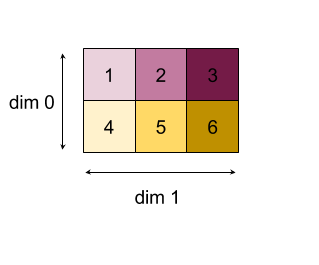
Resultados de reducir las dimensiones 0 o 1 con una función "add":
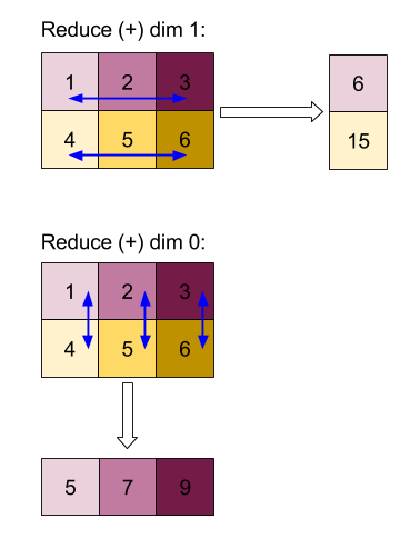
Ten en cuenta que ambos resultados de reducción son arrays 1D. El diagrama muestra uno como columna y otro como fila solo para mayor conveniencia visual.
Para ver un ejemplo más complejo, aquí hay un array en 3D. Su clasificación es 3, dimensión 0 de tamaño 4, dimensión 1 de tamaño 2 y dimensión 2 de tamaño 3. Para simplificar, los valores del 1 al 6 se replican en la dimensión 0.
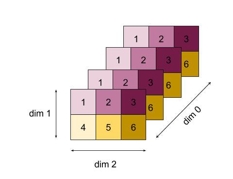
Al igual que en el ejemplo en 2D, podemos reducir solo una dimensión. Si reducimos la dimensión 0, por ejemplo, obtenemos un array de rango-2 en el que todos los valores de la dimensión 0 se pliegan en un escalar:
|  4   8  12 |
| 16  20  24 |
Si reducimos la dimensión 2, también obtenemos un array de rango 2 en el que todos los valores de la dimensión 2 se plegaron en un escalar:
| 6  15 |
| 6  15 |
| 6  15 |
| 6  15 |
Ten en cuenta que el orden relativo entre las dimensiones restantes de la entrada se conserva en la salida, pero es posible que se asignen números nuevos a algunas dimensiones (debido a que la clasificación cambia).
También podemos reducir varias dimensiones. Si se reducen las dimensiones 0 y 1, se produce el array 1D [20, 28, 36].
Cuando reduces el array 3D en todas sus dimensiones, se produce el 84 escalar.
Reductor variable
Cuando es N > 1, la aplicación de la función de reducción es un poco más compleja, ya que se aplica simultáneamente a todas las entradas. Los operandos se suministran al cálculo en el siguiente orden:
- Ejecutando un valor reducido para el primer operando
- ...
- Ejecutando valor reducido para el operando enésimo
- Valor de entrada para el primer operando
- ...
- Valor de entrada para el operando enésimo
Por ejemplo, considera la siguiente función de reducción, que se puede usar para calcular el máximo y el argmax de un array de 1D en paralelo:
f: (Float, Int, Float, Int) -> Float, Int
f(max, argmax, value, index):
  if value >= max:
    return (value, index)
  else:
    return (max, argmax)
Para los arrays de entrada 1D V = Float[N], K = Int[N] y los valores init I_V = Float, I_K = Int, el resultado f_(N-1) de la reducción en la única dimensión de entrada es equivalente a la siguiente aplicación recursiva:
f_0 = f(I_V, I_K, V_0, K_0)
f_1 = f(f_0.first, f_0.second, V_1, K_1)
...
f_(N-1) = f(f_(N-2).first, f_(N-2).second, V_(N-1), K_(N-1))
Si aplicas esta reducción a un array de valores y un array de índices secuenciales (es decir, iota), se realizará una iteración en los arrays y se mostrará una tupla con el valor máximo y el índice coincidente.
ReducePrecision
Consulta también XlaBuilder::ReducePrecision.
Modela el efecto de convertir los valores de punto flotante a un formato de menor precisión (como IEEE-FP16) y de vuelta al formato original. La cantidad de bits exponentes y mantisas en el formato de menor precisión se puede especificar de manera arbitraria, aunque es posible que todos los tamaños de bits no sean compatibles con todas las implementaciones de hardware.
ReducePrecision(operand, mantissa_bits, exponent_bits)
| Argumentos | Tipo | Semántica |
|---|---|---|
operand |
XlaOp |
array de tipo de punto flotante T. |
exponent_bits |
int32 |
cantidad de bits exponentes en formato de menor precisión |
mantissa_bits |
int32 |
cantidad de bits de mantisa en un formato de menor precisión |
El resultado es un array de tipo T. Los valores de entrada se redondean al valor más cercano representable con la cantidad determinada de bits de mantisa (con la semántica de "empates a pares"), y cualquier valor que exceda el rango especificado por la cantidad de bits exponentes se restringe al infinito positivo o negativo. Se conservan los valores NaN, aunque se pueden convertir en valores NaN canónicos.
El formato de menor precisión debe tener al menos un bit exponente (para distinguir un valor cero de un infinito, ya que ambos tienen una mantisa cero) y debe tener un número no negativo de bits mantisa. La cantidad de bits de exponente o de mantisa puede exceder el valor correspondiente para el tipo T. La parte correspondiente de la conversión es simplemente una no-op.
ReduceScatter
Consulta también XlaBuilder::ReduceScatter.
ReduceScatter es una operación colectiva que realiza un AllReduce y, luego, dispersa el resultado dividiéndolo en bloques shard_count a lo largo de scatter_dimension, y la réplica i en el grupo de réplicas recibe el fragmento ith.
ReduceScatter(operand, computation, scatter_dim, shard_count,
replica_group_ids, channel_id)
| Argumentos | Tipo | Semántica |
|---|---|---|
operand |
XlaOp |
Es un array o una tupla no vacía de arrays que se reducirán en las réplicas. |
computation |
XlaComputation |
Cálculo de la reducción |
scatter_dimension |
int64 |
Dimensión que se dispersará. |
shard_count |
int64 |
Cantidad de bloques para dividir scatter_dimension |
replica_groups |
vector de vectores de int64 |
Grupos entre los que se realizan las reducciones |
channel_id |
int64 opcional |
ID de canal opcional para la comunicación entre módulos |
- Cuando
operandes una tupla de arreglos, la reducción de dispersión se realiza en cada elemento de la tupla. replica_groupses una lista de grupos de réplica entre los que se realiza la reducción (el ID de réplica de la réplica actual se puede recuperar medianteReplicaId). El orden de las réplicas en cada grupo determina el orden en el que se dispersará el resultado de la reducción total.replica_groupsdebe estar vacío (en ese caso, todas las réplicas pertenecen a un solo grupo) o contener la misma cantidad de elementos que la cantidad de réplicas. Cuando hay más de un grupo de réplicas, todos deben ser del mismo tamaño. Por ejemplo,replica_groups = {0, 2}, {1, 3}realiza una reducción entre las réplicas0y2, y1y3, y, luego, dispersa el resultado.shard_countes el tamaño de cada grupo de réplicas. Necesitamos esto en los casos en quereplica_groupsesté vacío. Sireplica_groupsno está vacío,shard_countdebe ser igual al tamaño de cada grupo de réplicas.channel_idse usa para la comunicación entre módulos: solo las operacionesreduce-scattercon el mismochannel_idpueden comunicarse entre sí.
La forma de salida es la de entrada con el elemento scatter_dimension hecho shard_count veces más pequeño. Por ejemplo, si hay dos réplicas y el operando tiene el valor [1.0, 2.25] y [3.0, 5.25] respectivamente en las dos réplicas, el valor de salida de esta op en la que scatter_dim es 0 será [4.0] para la primera réplica y [7.5] para la segunda.
ReduceWindow
Consulta también XlaBuilder::ReduceWindow.
Aplica una función de reducción a todos los elementos en cada ventana de una secuencia de N arrays multidimensionales, lo que produce una única o una tupla de N arrays multidimensionales como resultado. Cada array de salida tiene la misma cantidad de elementos que la cantidad de posiciones válidas de la ventana. Una capa de reducción se puede expresar como ReduceWindow. Al igual que Reduce, al objeto computation aplicado siempre se le pasa init_values en el lado izquierdo.
ReduceWindow(operands..., init_values..., computation, window_dimensions,
window_strides, padding)
| Argumentos | Tipo | Semántica |
|---|---|---|
operands |
N XlaOps |
Es una secuencia de N arrays multidimensionales de tipos T_0,..., T_{N-1}, cada uno de los cuales representa el área base en la que se coloca la ventana. |
init_values |
N XlaOps |
Los N valores iniciales para la reducción, uno para cada uno de los N operandos. Consulta Reducir para obtener más detalles. |
computation |
XlaComputation |
Función de reducción de tipo T_0, ..., T_{N-1}, T_0, ..., T_{N-1} -> Collate(T_0, ..., T_{N-1}), para aplicar a elementos en cada ventana de todos los operandos de entrada. |
window_dimensions |
ArraySlice<int64> |
array de números enteros para valores de dimensión de ventana |
window_strides |
ArraySlice<int64> |
array de números enteros para los valores de segmento de ventana |
base_dilations |
ArraySlice<int64> |
array de números enteros para los valores de dilatación base |
window_dilations |
ArraySlice<int64> |
array de números enteros para valores de dilatación de ventana |
padding |
Padding |
tipo de relleno para la ventana (Padding::kSame, que se rellena para tener la misma forma de salida que la entrada si el stride es 1, o Padding::kValid, que no usa relleno y “detiene” la ventana cuando ya no encaja) |
Aquí:
- N debe ser mayor o igual que 1.
- Todos los arrays de entrada deben tener las mismas dimensiones.
- Si es
N = 1,Collate(T)esT. - Si es
N > 1,Collate(T_0, ..., T_{N-1})es una tupla de elementosNde tipo(T0,...T{N-1}).
Debajo del código y la figura, se muestra un ejemplo del uso de ReduceWindow. La entrada es una matriz de tamaño [4x6], y tanto window_dimensions como window_stride_dimensions son [2x3].
// Create a computation for the reduction (maximum).
XlaComputation max;
{
  XlaBuilder builder(client_, "max");
  auto y = builder.Parameter(0, ShapeUtil::MakeShape(F32, {}), "y");
  auto x = builder.Parameter(1, ShapeUtil::MakeShape(F32, {}), "x");
  builder.Max(y, x);
  max = builder.Build().value();
}

// Create a ReduceWindow computation with the max reduction computation.
XlaBuilder builder(client_, "reduce_window_2x3");
auto shape = ShapeUtil::MakeShape(F32, {4, 6});
auto input = builder.Parameter(0, shape, "input");
builder.ReduceWindow(
    input,
    /*init_val=*/builder.ConstantLiteral(LiteralUtil::MinValue(F32)),
    *max,
    /*window_dimensions=*/{2, 3},
    /*window_stride_dimensions=*/{2, 3},
    Padding::kValid);
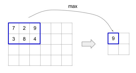
El segmento de 1 en una dimensión especifica que la posición de una ventana en la dimensión se encuentra a 1 elemento de distancia de la ventana adyacente. Para especificar que ninguna ventana se superponga entre sí, window_stride_dimensions debe ser igual a window_dimensions. En la siguiente figura, se ilustra el uso de dos valores de zancada diferentes. El padding se aplica a cada dimensión de la entrada, y los cálculos son los mismos que si la entrada tuviera las dimensiones que tenía después del padding.
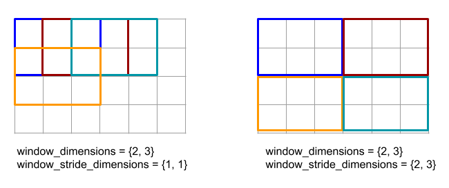
Para un ejemplo de padding no trivial, considera calcular el mínimo de ventana reducida (el valor inicial es MAX_FLOAT) con la dimensión 3 y el segmento 2 sobre el array de entrada [10000, 1000, 100, 10, 1]. El relleno kValid calcula los mínimos en dos ventanas válidas: [10000, 1000, 100] y [100, 10, 1], lo que da como resultado el [100, 1] de salida. El padding kSame primero rellena el array para que la forma después de la ventana de reducción sea la misma que la entrada para el segmento uno. Para ello, agrega elementos iniciales en ambos lados y obtén [MAX_VALUE, 10000, 1000, 100, 10, 1,
MAX_VALUE]. La ejecución de reduce-window sobre el array con padding opera en tres ventanas [MAX_VALUE, 10000, 1000], [1000, 100, 10], [10, 1, MAX_VALUE] y produce [1000, 10, 1].
El orden de evaluación de la función de reducción es arbitrario y puede ser no determinista. Por lo tanto, la función de reducción no debe ser demasiado sensible a la reasociación. Consulta el debate sobre la asociatividad en el contexto de Reduce para obtener más detalles.
ReplicaId
Consulta también XlaBuilder::ReplicaId.
Muestra el ID único (escalar U32) de la réplica.
ReplicaId()
El ID único de cada réplica es un número entero sin firma en el intervalo [0, N), en el que N es la cantidad de réplicas. Dado que todas las réplicas ejecutan el mismo programa, una llamada a ReplicaId() en el programa mostrará un valor diferente en cada réplica.
Reshape
Consulta también XlaBuilder::Reshape y la operación Collapse.
Cambia la forma de las dimensiones de un array a una configuración nueva.
Reshape(operand, new_sizes)
Reshape(operand, dimensions, new_sizes)
| Argumentos | Tipo | Semántica |
|---|---|---|
operand |
XlaOp |
array de tipo T |
dimensions |
Vector de int64 |
orden en que se contraen las dimensiones |
new_sizes |
Vector de int64 |
vector de tamaños de nuevas dimensiones |
Conceptualmente, el cambio de forma primero aplana un array en un vector unidimensional de valores de datos y, luego, define mejor este vector con una nueva forma. Los argumentos de entrada son un arreglo arbitrario de tipo T, un vector constante de tiempo de compilación de índices de dimensión y un vector constante de tiempo de compilación de tamaños de dimensión para el resultado.
Los valores en el vector dimension, si se proporcionan, deben ser una permutación de todas las dimensiones de T; el valor predeterminado si no se proporciona es {0, ..., rank - 1}. El orden de las dimensiones en dimensions es desde la dimensión más lenta que varía (la más importante) hasta la que varía más rápida (la mayor parte de la menor) en el nido de bucles, que contrae el array de entrada en una sola dimensión. El vector new_sizes determina el tamaño del array de salida. El valor en el índice 0 de new_sizes es el tamaño de la dimensión 0, el valor en el índice 1 es el tamaño de la dimensión 1, y así sucesivamente. El producto de las dimensiones de new_size debe ser igual al producto de los tamaños de dimensión del operando. Cuando defines mejor el array contraído en el array multidimensional definido por new_sizes, las dimensiones en new_sizes se ordenan de la variable más lenta (la mayor parte) a la más rápida (la más pequeña).
Por ejemplo, supongamos que v es un array de 24 elementos:
let v = f32[4x2x3] { { {10, 11, 12}, {15, 16, 17} },
                    { {20, 21, 22}, {25, 26, 27} },
                    { {30, 31, 32}, {35, 36, 37} },
                    { {40, 41, 42}, {45, 46, 47} } };

In-order collapse:
let v012_24 = Reshape(v, {0,1,2}, {24});
then v012_24 == f32[24] {10, 11, 12, 15, 16, 17, 20, 21, 22, 25, 26, 27,
                         30, 31, 32, 35, 36, 37, 40, 41, 42, 45, 46, 47};

let v012_83 = Reshape(v, {0,1,2}, {8,3});
then v012_83 == f32[8x3] { {10, 11, 12}, {15, 16, 17},
                          {20, 21, 22}, {25, 26, 27},
                          {30, 31, 32}, {35, 36, 37},
                          {40, 41, 42}, {45, 46, 47} };

Out-of-order collapse:
let v021_24 = Reshape(v, {1,2,0}, {24});
then v012_24 == f32[24]  {10, 20, 30, 40, 11, 21, 31, 41, 12, 22, 32, 42,
                          15, 25, 35, 45, 16, 26, 36, 46, 17, 27, 37, 47};

let v021_83 = Reshape(v, {1,2,0}, {8,3});
then v021_83 == f32[8x3] { {10, 20, 30}, {40, 11, 21},
                          {31, 41, 12}, {22, 32, 42},
                          {15, 25, 35}, {45, 16, 26},
                          {36, 46, 17}, {27, 37, 47} };


let v021_262 = Reshape(v, {1,2,0}, {2,6,2});
then v021_262 == f32[2x6x2] { { {10, 20}, {30, 40},
                              {11, 21}, {31, 41},
                              {12, 22}, {32, 42} },
                             { {15, 25}, {35, 45},
                              {16, 26}, {36, 46},
                              {17, 27}, {37, 47} } };
Como caso especial, el cambio de forma puede transformar un array de un solo elemento en un escalar y viceversa. Por ejemplo,
Reshape(f32[1x1] { {5} }, {0,1}, {}) == 5;
Reshape(5, {}, {1,1}) == f32[1x1] { {5} };
Rev. (inversa)
Consulta también XlaBuilder::Rev.
Rev(operand, dimensions)
| Argumentos | Tipo | Semántica |
|---|---|---|
operand |
XlaOp |
array de tipo T |
dimensions |
ArraySlice<int64> |
dimensiones para revertir |
Invierte el orden de los elementos en el array operand a lo largo del dimensions especificado, lo que genera un array de salida de la misma forma. Cada elemento del arreglo de operando en un índice multidimensional se almacena en el arreglo de salida en un índice transformado. El índice multidimensional se transforma mediante la inversión del índice en cada dimensión que se revertirá (es decir, si una dimensión de tamaño N es una de las dimensiones inversas, su índice i se transforma en N - 1 - i).
Un uso de la operación Rev es revertir el array de pesos de convolución a lo largo de las dos dimensiones de ventana durante el cálculo de gradientes en redes neuronales.
RngNormal
Consulta también XlaBuilder::RngNormal.
Construye una salida de una forma determinada con números aleatorios generados según la \(N(\mu, \sigma)\) distribución normal. Los parámetros \(\mu\) , \(\sigma\)y la forma de salida deben tener un tipo elemental de punto flotante. Además, los parámetros deben tener un valor escalar.
RngNormal(mu, sigma, shape)
| Argumentos | Tipo | Semántica |
|---|---|---|
mu |
XlaOp |
Escalar de tipo T que especifica la media de los números generados |
sigma |
XlaOp |
Escalar de tipo T que especifica la desviación estándar del elemento generado |
shape |
Shape |
Forma de salida de tipo T |
RngUniform
Consulta también XlaBuilder::RngUniform.
Construye una salida de una forma determinada con números aleatorios generados a partir de la distribución uniforme durante el intervalo \([a,b)\). Los parámetros y el tipo de elemento de salida deben ser de tipo booleano, integral o de punto flotante, y los tipos deben ser coherentes. En la actualidad, los backends de CPU y GPU solo admiten F64, F32, F16, BF16, S64, U64, S32 y U32. Además, los parámetros deben tener un valor escalar. Si es \(b <= a\) , el resultado está definido por la implementación.
RngUniform(a, b, shape)
| Argumentos | Tipo | Semántica |
|---|---|---|
a |
XlaOp |
Escalar de tipo T que especifica un límite inferior de intervalo |
b |
XlaOp |
Escalar de tipo T que especifica el límite superior de intervalo |
shape |
Shape |
Forma de salida de tipo T |
RngBitGenerator
Genera una salida con una forma determinada llena de bits aleatorios uniformes mediante el uso del algoritmo especificado (o el valor predeterminado del backend) y muestra un estado actualizado (con la misma forma que el estado inicial) y los datos aleatorios generados.
El estado inicial es el estado inicial de la generación actual de números aleatorios. Este, la forma requerida y los valores válidos dependen del algoritmo utilizado.
Se garantiza que el resultado es una función determinista del estado inicial, pero no se garantiza que lo sea entre los backends y las diferentes versiones del compilador.
RngBitGenerator(algorithm, key, shape)
| Argumentos | Tipo | Semántica |
|---|---|---|
algorithm |
RandomAlgorithm |
Se usará el algoritmo PRNG. |
initial_state |
XlaOp |
Estado inicial del algoritmo PRNG |
shape |
Shape |
Forma de salida para los datos generados. |
Valores disponibles para algorithm:
rng_default: Algoritmo específico de backend con requisitos de forma específicos de backend.rng_three_fry: Algoritmo de PRNG basado en contador de ThreeFry. La formainitial_stateesu64[2]con valores arbitrarios. Salmon et al. SC 2011. Números aleatorios paralelos: tan sencillos como 1, 2, 3rng_philox: Es el algoritmo Philox para generar números aleatorios en paralelo. La formainitial_stateesu64[3]con valores arbitrarios. Salmon et al. SC 2011. Números aleatorios paralelos: tan sencillos como 1, 2, 3
Dispersión
La operación de dispersión de XLA genera una secuencia de resultados que son los valores del arreglo de entrada operands, con varias porciones (en los índices especificados por scatter_indices) actualizadas con la secuencia de valores en updates mediante update_computation.
Consulta también XlaBuilder::Scatter.
scatter(operands..., scatter_indices, updates..., update_computation,
index_vector_dim, update_window_dims, inserted_window_dims,
scatter_dims_to_operand_dims)
| Argumentos | Tipo | Semántica |
|---|---|---|
operands |
Secuencia de N XlaOp |
N arrays de tipos T_0, ..., T_N en los que se dispersarán. |
scatter_indices |
XlaOp |
Arreglo que contiene los índices iniciales de las porciones que deben dispersarse. |
updates |
Secuencia de N XlaOp |
N arrays de tipos T_0, ..., T_N. updates[i] contiene los valores que se deben usar para la dispersión operands[i]. |
update_computation |
XlaComputation |
Cálculo que se usará para combinar los valores existentes en el array de entrada y las actualizaciones durante la dispersión. Este cálculo debe ser del tipo T_0, ..., T_N, T_0, ..., T_N -> Collate(T_0, ..., T_N). |
index_vector_dim |
int64 |
Es la dimensión de scatter_indices que contiene los índices iniciales. |
update_window_dims |
ArraySlice<int64> |
Es el conjunto de dimensiones en forma updates que son dimensiones de ventana. |
inserted_window_dims |
ArraySlice<int64> |
El conjunto de dimensiones de la ventana que se deben insertar en la forma updates |
scatter_dims_to_operand_dims |
ArraySlice<int64> |
Se asigna un mapa de dimensiones desde los índices de dispersión al espacio de índice de operando. Este array se interpreta como la asignación de i a scatter_dims_to_operand_dims[i] . Tiene que ser uno a uno y total. |
indices_are_sorted |
bool |
Indica si se garantiza que los índices estén ordenados por el emisor. |
Aquí:
- N debe ser mayor o igual que 1.
operands[0], ...,operands[N-1] deben tener las mismas dimensiones.updates[0], ...,updates[N-1] deben tener las mismas dimensiones.- Si es
N = 1,Collate(T)esT. - Si es
N > 1,Collate(T_0, ..., T_N)es una tupla de elementosNde tipoT.
Si index_vector_dim es igual a scatter_indices.rank, consideramos implícitamente que scatter_indices tiene una dimensión 1 final.
Definimos update_scatter_dims de tipo ArraySlice<int64> como el conjunto de dimensiones en forma de updates que no están en update_window_dims, en orden ascendente.
Los argumentos de dispersión deben seguir estas restricciones:
Cada array
updatesdebe tener la clasificaciónupdate_window_dims.size + scatter_indices.rank - 1.Los límites de la dimensión
ien cada arrayupdatesdeben cumplir con lo siguiente:- Si
iestá presente enupdate_window_dims(es decir, igual aupdate_window_dims[k] para algunosk), el límite de la dimensiónienupdatesno debe exceder el límite correspondiente deoperanddespués de considerarinserted_window_dims(es decir,adjusted_window_bounds[k], dondeadjusted_window_boundscontiene los límites deoperandsin los límites de los índicesinserted_window_dims). - Si
iestá presente enupdate_scatter_dims(es decir, igual aupdate_scatter_dims[k] para algunosk), el límite de la dimensiónienupdatesdebe ser igual al límite correspondiente descatter_indices, y se omiteindex_vector_dim(es decir,scatter_indices.shape.dims[k], sik<index_vector_dimyscatter_indices.shape.dims[k+1] en caso contrario).
- Si
update_window_dimsdebe estar en orden ascendente, no tener números de dimensión repetidos y estar dentro del rango[0, updates.rank).inserted_window_dimsdebe estar en orden ascendente, no tener números de dimensión repetidos y estar dentro del rango[0, operand.rank).operand.rankdebe ser igual a la suma deupdate_window_dims.sizeyinserted_window_dims.size.scatter_dims_to_operand_dims.sizedebe ser igual ascatter_indices.shape.dims[index_vector_dim] y sus valores deben estar en el rango[0, operand.rank).
Para un índice U determinado en cada array updates, el índice correspondiente I en el array operands correspondiente al que se debe aplicar esta actualización se calcula de la siguiente manera:
- Deja que
G= {U[k] parakenupdate_scatter_dims}. UsaGpara buscar un vector de índiceSen el arrayscatter_indicesde modo queS[i] =scatter_indices[Combine(G,i)], en el que Combine(A, b) inserta b en las posicionesindex_vector_dimen A. - Crea un índice
SinenoperandmedianteSmediante la dispersiónScon el mapascatter_dims_to_operand_dims. Más formalmente:Sin[scatter_dims_to_operand_dims[k]] =S[k] sik<scatter_dims_to_operand_dims.size.Sin[_] =0de lo contrario.
- Crea un índice
Winen cada arrayoperands. Para ello, distribuye los índices enupdate_window_dimsenUde acuerdo coninserted_window_dims. Más formalmente:Win[window_dims_to_operand_dims(k)] =U[k] sikestá enupdate_window_dims, dondewindow_dims_to_operand_dimses la función monótona con el dominio [0,update_window_dims.size) y el rango [0,operand.rank) \inserted_window_dims. (Por ejemplo, siupdate_window_dims.sizees4,operand.rankes6yinserted_window_dimses {0,2}, entonceswindow_dims_to_operand_dimses {0→1,1→3,2→4,3→5}).Win[_] =0de lo contrario.
IesWin+Sin, donde + representa la suma a nivel de los elementos.
En resumen, la operación de dispersión se puede definir de la siguiente manera.
- Inicializa
outputconoperands, es decir, para todos los índicesJ, para todos los índicesOdel arrayoperands[J]:
output[J][O] =operands[J][O] - Para cada índice
Uen el arrayupdates[J] y el índice correspondienteOen el arrayoperand[J], siOes un índice válido paraoutput:
(output[0][O], ...,output[N-1][O]) =update_computation(output[0][O], ..., ,output[N-1][O],updates[0][U], ...,updates[N-1][U])
El orden en el que se aplican las actualizaciones no es determinista. Por lo tanto, cuando varios índices de updates hagan referencia al mismo índice en operands, el valor correspondiente de output no será determinista.
Ten en cuenta que el primer parámetro que se pasa a update_computation siempre será el valor actual del array output y el segundo siempre será el valor del array updates. Esto es importante en particular para los casos en los que update_computation no es conmutativo.
Si se configura indices_are_sorted como verdadero, XLA puede suponer que el usuario ordena start_indices (en orden ascendente start_index_map). Si no lo son, la implementación se define en la semántica.
Informalmente, la operación de dispersión puede verse como una operación inversa de la operación de recopilación, es decir, la operación de dispersión actualiza los elementos en la entrada que extrae la operación de recopilación correspondiente.
Para obtener una descripción informal detallada y ejemplos, consulta la sección "Descripción informal" en Gather.
Seleccionar
Consulta también XlaBuilder::Select.
Construye un arreglo de salida a partir de elementos de dos arreglos de entrada, en función de los valores de un arreglo de predicado.
Select(pred, on_true, on_false)
| Argumentos | Tipo | Semántica |
|---|---|---|
pred |
XlaOp |
array de tipo PRED |
on_true |
XlaOp |
array de tipo T |
on_false |
XlaOp |
array de tipo T |
Los arrays on_true y on_false deben tener la misma forma. Esta también es la forma del array de salida. El array pred debe tener la misma dimensionalidad que on_true y on_false, con el tipo de elemento PRED.
Para cada elemento P de pred, el elemento correspondiente del array de salida se toma de on_true si el valor de P es true y de on_false si el valor de P es false. Como una forma restringida de transmisión, pred puede ser un escalar de tipo PRED. En este caso, el array de salida se toma por completo de on_true si pred es true y de on_false si pred es false.
Ejemplo con pred no escalar:
let pred: PRED[4] = {true, false, false, true};
let v1: s32[4] = {1, 2, 3, 4};
let v2: s32[4] = {100, 200, 300, 400};
==>
Select(pred, v1, v2) = s32[4]{1, 200, 300, 4};
Ejemplo con pred escalar:
let pred: PRED = true;
let v1: s32[4] = {1, 2, 3, 4};
let v2: s32[4] = {100, 200, 300, 400};
==>
Select(pred, v1, v2) = s32[4]{1, 2, 3, 4};
Se admiten selecciones entre tuplas. Para este propósito, las tuplas se consideran tipos escalares. Si on_true y on_false son tuplas (que deben tener la misma forma), pred debe ser un escalar de tipo PRED.
SelectAndScatter
Consulta también XlaBuilder::SelectAndScatter.
Esta operación puede considerarse como una operación compuesta que primero calcula ReduceWindow en el array operand para seleccionar un elemento de cada ventana y, luego, dispersa el array source en los índices de los elementos seleccionados para construir un array de salida con la misma forma que el array de operando. La función binaria select se usa para seleccionar un elemento de cada ventana aplicándolo en cada ventana, y se llama con la propiedad de que el vector de índice del primer parámetro es lexicográficamente menor que el vector de índice del segundo parámetro. La función select muestra true si el primer parámetro está seleccionado y false si se selecciona el segundo parámetro, y la función debe contener la transitividad (es decir, si select(a, b) y select(b, c) son true, entonces select(a, c) también es true) para que el elemento seleccionado no dependa del orden de los elementos recorridos para una ventana determinada.
La función scatter se aplica a cada índice seleccionado en el array de salida. Se necesitan dos parámetros escalares:
- Valor actual en el índice seleccionado en el array de salida
- El valor de dispersión de
sourceque se aplica al índice seleccionado
Combina los dos parámetros y muestra un valor escalar que se usa para actualizar el valor en el índice seleccionado en el arreglo de salida. Inicialmente, todos los índices del arreglo de salida se configuran en init_value.
El array de salida tiene la misma forma que el array operand, y el array source debe tener la misma forma que el resultado de aplicar una operación ReduceWindow en el array operand. Se puede usar SelectAndScatter para la propagación inversa de los valores de gradiente de una capa de reducción en una red neuronal.
SelectAndScatter(operand, select, window_dimensions, window_strides,
padding, source, init_value, scatter)
| Argumentos | Tipo | Semántica |
|---|---|---|
operand |
XlaOp |
array de tipo T sobre el que se deslizan las ventanas |
select |
XlaComputation |
Cálculo binario de tipo T, T -> PRED, para aplicar a todos los elementos en cada ventana; muestra true si se selecciona el primer parámetro y false si se selecciona el segundo parámetro |
window_dimensions |
ArraySlice<int64> |
array de números enteros para valores de dimensión de ventana |
window_strides |
ArraySlice<int64> |
array de números enteros para los valores de segmento de ventana |
padding |
Padding |
Tipo de padding para la ventana (Padding::kSame o Padding::kValid) |
source |
XlaOp |
array de tipo T con los valores para dispersar |
init_value |
XlaOp |
valor escalar de tipo T para el valor inicial del array de salida |
scatter |
XlaComputation |
Cálculo binario de tipo T, T -> T, para aplicar cada elemento de origen de dispersión con su elemento de destino |
En la siguiente figura, se muestran ejemplos del uso de SelectAndScatter, con la función select que calcula el valor máximo entre sus parámetros. Ten en cuenta que, cuando las ventanas se superponen, como se muestra en la siguiente figura (2), es posible que diferentes ventanas seleccionen un índice del array operand varias veces. En la figura, se selecciona el elemento de valor 9 en las dos ventanas superiores (azul y rojo) y la función scatter de adición binaria produce el elemento de resultado del valor 8 (2 + 6).
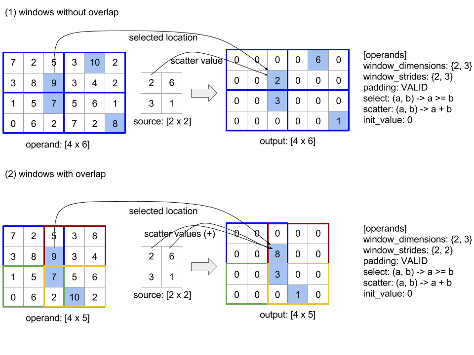
El orden de evaluación de la función scatter es arbitrario y puede ser no determinista. Por lo tanto, la función scatter no debe ser demasiado sensible a la reasociación. Consulta el debate sobre la asociatividad en el contexto de Reduce para obtener más detalles.
Enviar
Consulta también XlaBuilder::Send.
Send(operand, channel_handle)
| Argumentos | Tipo | Semántica |
|---|---|---|
operand |
XlaOp |
datos para enviar (matriz de tipo T) |
channel_handle |
ChannelHandle |
identificador único para cada par de envío y recepción |
Envía los datos del operando dados a una instrucción Recv en otro cálculo que comparte el mismo controlador de canal. No muestra ningún dato.
Al igual que la operación Recv, la API de cliente de la operación Send representa la comunicación síncrona y se divide internamente en 2 instrucciones HLO (Send y SendDone) para habilitar las transferencias de datos asíncronas. Consulta también HloInstruction::CreateSend y HloInstruction::CreateSendDone.
Send(HloInstruction operand, int64 channel_id)
Inicia una transferencia asíncrona del operando a los recursos asignados por la instrucción Recv con el mismo ID de canal. Muestra un contexto, que se usa con la siguiente instrucción SendDone para esperar que se complete la transferencia de datos. El contexto es una tupla de {operando (forma), identificador de solicitud (U32)} y solo se puede usar con una instrucción SendDone.
SendDone(HloInstruction context)
En un contexto creado por una instrucción Send, espera a que se complete la transferencia de datos. La instrucción no devuelve ningún dato.
Programación de instrucciones del canal
El orden de ejecución de las 4 instrucciones para cada canal (Recv, RecvDone, Send, SendDone) es el siguiente:
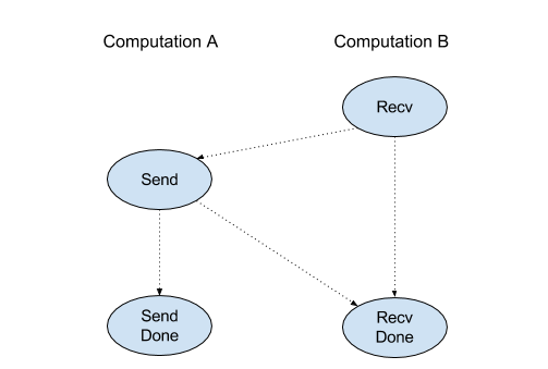
Recvocurre antes delSendSendocurre antes delRecvDoneRecvocurre antes delRecvDoneSendocurre antes delSendDone
Cuando los compiladores de backend generan un programa lineal para cada procesamiento que se comunica a través de instrucciones de canal, no debe haber ciclos a través de los cálculos. Por ejemplo, los siguientes programas generan interbloqueos.
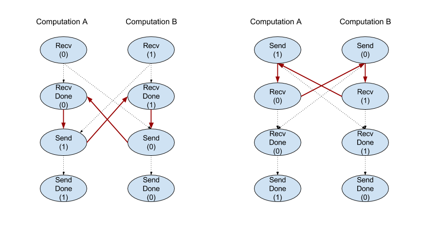
Porción
Consulta también XlaBuilder::Slice.
Con la segmentación, se extrae un subarreglo del array de entrada. El subarreglo es del mismo rango que la entrada y contiene los valores dentro de un cuadro delimitador dentro del array de entrada, en el que las dimensiones y los índices del cuadro se proporcionan como argumentos para la operación de división.
Slice(operand, start_indices, limit_indices, strides)
| Argumentos | Tipo | Semántica |
|---|---|---|
operand |
XlaOp |
Arreglo n-dimensional de tipo T |
start_indices |
ArraySlice<int64> |
Lista de N números enteros que contienen los índices iniciales de la porción para cada dimensión. Los valores deben ser mayores o iguales que cero. |
limit_indices |
ArraySlice<int64> |
Lista de N números enteros que contienen los índices finales (exclusivos) de la porción de cada dimensión. Cada valor debe ser mayor o igual que el valor de start_indices respectivo de la dimensión, así como menor o igual que su tamaño. |
strides |
ArraySlice<int64> |
Lista de N números enteros que deciden el segmento de entrada de la porción. La porción selecciona cada elemento strides[d] en la dimensión d. |
Ejemplo unidimensional:
let a = {0.0, 1.0, 2.0, 3.0, 4.0}
Slice(a, {2}, {4}) produces:
  {2.0, 3.0}
Ejemplo bidimensional:
let b =
 { {0.0,  1.0,  2.0},
   {3.0,  4.0,  5.0},
   {6.0,  7.0,  8.0},
   {9.0, 10.0, 11.0} }

Slice(b, {2, 1}, {4, 3}) produces:
  { { 7.0,  8.0},
    {10.0, 11.0} }
Ordenar
Consulta también XlaBuilder::Sort.
Sort(operands, comparator, dimension, is_stable)
| Argumentos | Tipo | Semántica |
|---|---|---|
operands |
ArraySlice<XlaOp> |
Los operandos para ordenar. |
comparator |
XlaComputation |
Cálculo del comparador que se usará. |
dimension |
int64 |
La dimensión en la que se ordenará. |
is_stable |
bool |
Si se debe usar el ordenamiento estable. |
Si solo se proporciona un operando:
Si el operando es un tensor de rango-1 (un array), el resultado es un array ordenado. Si deseas ordenar el array en orden ascendente, el comparador debe realizar una comparación de menor que. De manera formal, después de ordenar el array, conserva todas las posiciones de índice
i, jconi < jque seancomparator(value[i], value[j]) = comparator(value[j], value[i]) = falseocomparator(value[i], value[j]) = true.Si el operando tiene una clasificación más alta, se ordena según la dimensión proporcionada. Por ejemplo, para un tensor de rango-2 (una matriz), un valor de dimensión de
0ordenará de forma independiente cada columna, y un valor de dimensión de1ordenará cada fila de forma independiente. Si no se proporciona un número de dimensión, se elige la última dimensión de forma predeterminada. Para la dimensión que está ordenada, se aplica el mismo orden de clasificación que en el caso de rango-1.
Si se proporcionan operandos n > 1:
Todos los operandos
ndeben ser tensores con las mismas dimensiones. Los tipos de elementos de los tensores pueden ser diferentes.Todos los operandos se ordenan juntos, no de manera individual. Conceptualmente, los operandos se tratan como una tupla. Cuando se verifica si los elementos de cada operando en las posiciones de índice
iyjdeben intercambiarse, se llama al comparador con parámetros escalares2 * n, en el que el parámetro2 * kcorresponde al valor en la posiciónidel operandok-thy el parámetro2 * k + 1corresponde al valor en la posiciónjdel operandok-th. Por lo general, el comparador compara los parámetros2 * ky2 * k + 1entre sí, y es posible que use otros pares de parámetros como separadores de empate.El resultado es una tupla que consta de los operandos en orden (en la dimensión proporcionada, como se muestra más arriba). El operando
i-thde la tupla corresponde al operandoi-thde Sort.
Por ejemplo, si hay tres operandos operand0 = [3, 1], operand1 = [42, 50], operand2 = [-3.0, 1.1], y el comparador solo compara los valores de operand0 con un valor menor que, la salida del orden es la tupla ([1, 3], [50, 42], [1.1, -3.0]).
Si se configura is_stable como verdadero, se garantiza que la ordenación sea estable, es decir, si hay elementos que el comparador considera iguales, se conserva el orden relativo de los valores iguales. Dos elementos, e1 y e2, son iguales solo si comparator(e1, e2) = comparator(e2, e1) = false. De forma predeterminada, is_stable se configura como falso.
Transposición
Consulta también la operación tf.reshape.
Transpose(operand)
| Argumentos | Tipo | Semántica |
|---|---|---|
operand |
XlaOp |
El operando que se transpondrá. |
permutation |
ArraySlice<int64> |
Cómo permutar las dimensiones |
Permuta las dimensiones del operando con la permutación determinada, por lo tanto, ∀ i . 0 ≤ i < rank ⇒ input_dimensions[permutation[i]] = output_dimensions[i].
Es lo mismo que Reshape(operando, permutación, Permute(permutación, operand.shape.dimensions)).
TriangularSolve
Consulta también XlaBuilder::TriangularSolve.
Resuelve sistemas de ecuaciones lineales con matrices de coeficientes triangulares inferior o superior mediante sustitución hacia adelante o atrás. Cuando se transmite a través de dimensiones principales, esta rutina resuelve uno de los sistemas matriciales op(a) * x =
b o x * op(a) = b para la variable x, con a y b, en los que op(a) es op(a) = a, op(a) = Transpose(a) o op(a) = Conj(Transpose(a)).
TriangularSolve(a, b, left_side, lower, unit_diagonal, transpose_a)
| Argumentos | Tipo | Semántica |
|---|---|---|
a |
XlaOp |
un array de rango > 2 de un tipo complejo o de punto flotante con forma [..., M, M]. |
b |
XlaOp |
un array de rango > 2 del mismo tipo con forma [..., M, K] si left_side es verdadero, de lo contrario, [..., K, M]. |
left_side |
bool |
indica si se debe resolver un sistema con el formato op(a) * x = b (true) o x * op(a) = b (false). |
lower |
bool |
si se debe usar el triángulo superior o inferior de a. |
unit_diagonal |
bool |
Si es true, se supone que los elementos diagonales de a son 1 y no se accede a ellos. |
transpose_a |
Transpose |
ya sea para usar a tal como está, transponerlo o tomar su transposición conjugada. |
Los datos de entrada se leen solo desde el triángulo inferior/superior de a, según el valor de lower. Se ignoran los valores del otro triángulo. Los datos de salida se muestran en el mismo triángulo; los valores en el otro triángulo están definidos por la implementación y pueden ser cualquiera.
Si la clasificación de a y b es mayor que 2, se tratan como lotes de matrices, y todas, excepto las 2 dimensiones menores, son dimensiones de lote. a y b deben tener las mismas dimensiones de lote.
Tupla
Consulta también XlaBuilder::Tuple.
Es una tupla que contiene un número variable de controladores de datos, cada uno de los cuales tiene su propia forma.
Es similar a std::tuple en C++. Conceptualmente:
let v: f32[10] = f32[10]{0, 1, 2, 3, 4, 5, 6, 7, 8, 9};
let s: s32 = 5;
let t: (f32[10], s32) = tuple(v, s);
Se puede deconstruir las tuplas (se puede acceder a ellas) mediante la operación GetTupleElement.
Mientras que
Consulta también XlaBuilder::While.
While(condition, body, init)
| Argumentos | Tipo | Semántica |
|---|---|---|
condition |
XlaComputation |
XlaComputation de tipo T -> PRED que define la condición de finalización del bucle. |
body |
XlaComputation |
XlaComputation de tipo T -> T que define el cuerpo del bucle. |
init |
T |
Valor inicial para el parámetro de condition y body. |
Ejecuta el body de forma secuencial hasta que condition falla. Esto es similar a un bucle while típico en muchos otros lenguajes, excepto por las diferencias y restricciones que se mencionan a continuación.
- Un nodo
Whilemuestra un valor de tipoT, que es el resultado de la última ejecución debody. - La forma del tipo
Tse determina de forma estática y debe ser la misma en todas las iteraciones.
Los parámetros T de los cálculos se inicializan con el valor init en la primera iteración y se actualizan automáticamente al resultado nuevo desde body en cada iteración posterior.
Un caso de uso principal del nodo While es implementar la ejecución repetida del entrenamiento en redes neuronales. A continuación, se muestra un pseudocódigo simplificado con un gráfico que representa el cálculo. Puedes encontrar el código en while_test.cc.
El tipo T en este ejemplo es una Tuple que consta de un int32 para el recuento de iteraciones y un vector[10] para el acumulador. Para 1,000 iteraciones, el bucle continúa agregando un vector constante al acumulador.
// Pseudocode for the computation.
init = {0, zero_vector[10]} // Tuple of int32 and float[10].
result = init;
while (result(0) < 1000) {
  iteration = result(0) + 1;
  new_vector = result(1) + constant_vector[10];
  result = {iteration, new_vector};
}