
Poniżej opisujemy semantykę operacji zdefiniowanych w interfejsie XlaBuilder. Zwykle te operacje mapują działania „jeden do jednego” na operacje zdefiniowane w interfejsie RPC w xla_data.proto.
Uwaga na temat nomenklatury: uogólniony typ danych XLA to n-wymiarowa tablica przechowująca elementy jakiegoś typu (np. 32-bitowej zmiennoprzecinkowej). W dokumentacji argument tablica służy do oznaczania tablicy o dowolnych wymiarach. Dla wygody specjalne przypadki mają bardziej szczegółowe i znane nazwy. Na przykład wektor to tablica jednowymiarowa, a macierz to tablica dwuwymiarowa.
AfterAll
Zobacz też XlaBuilder::AfterAll.
AfterAll wykorzystuje zmienną liczbę tokenów i generuje jeden token. Tokeny to typy podstawowe, które można łączyć w wątki między operacjami powodującymi uboczne działania, aby wymusić kolejność. AfterAll może służyć do łączenia tokenów w celu zamawiania operacji po operacjach zestawu.
AfterAll(operands)
| Argumenty | Typ | Semantyka |
|---|---|---|
operands |
XlaOp |
zmienna liczba tokenów |
AllGather
Zobacz też XlaBuilder::AllGather.
Wykonuje konkatenację w replikach.
AllGather(operand, all_gather_dim, shard_count, replica_group_ids,
channel_id)
| Argumenty | Typ | Semantyka |
|---|---|---|
operand
|
XlaOp
|
Tablica konkatenacji w replikach |
all_gather_dim |
int64 |
Wymiar konkatenacji |
replica_groups
|
wektor wektorów int64 |
Grupy, między którymi przeprowadza się łączenie danych, |
channel_id
|
opcjonalnie: int64
|
Opcjonalny identyfikator kanału na potrzeby komunikacji między modułami |
replica_groupsto lista grup replik, między którymi przeprowadzana jest konkatenacja (identyfikator repliki bieżącej repliki można pobrać za pomocąReplicaId). Kolejność replik w każdej grupie określa kolejność, w której dane wejściowe znajdują się w wyniku.replica_groupsmusi być pusta (w tym przypadku wszystkie repliki należą do jednej grupy, uporządkowane od0doN - 1) lub zawierać tę samą liczbę elementów, co liczba replik. Na przykładreplica_groups = {0, 2}, {1, 3}wykonuje konkatenację między replikami0i2oraz1i3.shard_countto rozmiar każdej grupy replik. Jest on potrzebny w sytuacjach, gdy polereplica_groupsjest puste.channel_idsłuży do komunikacji między modułami: tylko operacjeall-gatherz tym samym atrybutemchannel_idmogą się ze sobą komunikować.
Kształt wyjściowy jest kształtem wejściowym, w którym all_gather_dim powiększył się shard_count razy. Jeśli na przykład są 2 repliki, a operand w obu replikach ma wartości [1.0, 2.5] i [3.0, 5.25], to wartość wyjściowa tej operacji, w której all_gather_dim to 0, będzie wynosić [1.0, 2.5, 3.0,
5.25] w obu replikach.
AllReduce
Zobacz też XlaBuilder::AllReduce.
Wykonuje niestandardowe obliczenia w replikach.
AllReduce(operand, computation, replica_group_ids, channel_id)
| Argumenty | Typ | Semantyka |
|---|---|---|
operand
|
XlaOp
|
Tablica lub niepusta krotka tablic, aby zmniejszyć liczbę replik |
computation |
XlaComputation |
Obliczanie redukcji |
replica_groups
|
wektor wektorów int64 |
Grupy, w których są stosowane redukcje |
channel_id
|
opcjonalnie: int64
|
Opcjonalny identyfikator kanału na potrzeby komunikacji między modułami |
- Gdy
operandjest kropką tablicy, jej całkowite zmniejszenie jest wykonywane w przypadku każdego jej elementu. replica_groupsto lista grup replik, w których jest przeprowadzana redukcja (identyfikator repliki bieżącej repliki można pobrać za pomocąReplicaId). Polereplica_groupsmusi być puste (w tym przypadku wszystkie repliki należą do jednej grupy) lub zawierać taką samą liczbę elementów jak liczba replik. Na przykładreplica_groups = {0, 2}, {1, 3}zmniejsza liczbę replik0i2oraz1i3.channel_idsłuży do komunikacji między modułami: tylko operacjeall-reducez tym samym atrybutemchannel_idmogą się ze sobą komunikować.
Kształt wyjściowy jest taki sam jak kształt wejściowy. Jeśli na przykład są 2 repliki, a operand ma wartości [1.0, 2.5] i [3.0, 5.25] odpowiednio w 2 replikach, wartość wyjściowa tej operacji i obliczenia sumy będą wynosić [4.0, 7.75] w obu replikach. Jeśli dane wejściowe są kropką, dane wyjściowe też są kropką.
Przetwarzanie wyniku AllReduce wymaga podania 1 danych wejściowych z każdej repliki, więc jeśli jedna replika uruchomi węzeł AllReduce więcej razy niż drugi, Poprzednia replika będzie czekać w nieskończoność. Ponieważ wszystkie repliki działają w ramach tego samego programu, nie ma wielu sposobów, aby tak się stało, ale jest możliwe, że stan pętli podczas zdarzenia zależy od danych z InFeed, a dodane dane powodują, że pętla „if” jest powtarzana częściej w przypadku jednej repliki.
AllToAll
Zobacz też XlaBuilder::AllToAll.
AllToAll to operacja zbiorcza, która wysyła dane ze wszystkich rdzeni do wszystkich rdzeni. Składa się z 2 faz:
- Faza rozproszenia. W każdym rdzeniu operand jest dzielony na
split_countliczby bloków wzdłużsplit_dimensions, a bloki są rozproszone na wszystkich rdzeniach, np. i-ty blok jest wysyłany do i-tego rdzenia. - Faza zbierania. Każdy rdzeń łączy odebrane bloki w elemencie
concat_dimension.
Rdzenie biorące udział w programie można skonfigurować przez:
replica_groups: każda grupa ReplicaGroup zawiera listę identyfikatorów replik biorących udział w obliczeniach (identyfikator repliki bieżącej repliki można pobrać za pomocąReplicaId). Parametr AllToAll zostanie zastosowany w podgrupach w określonej kolejności. Na przykładreplica_groups = { {1,2,3}, {4,5,0} }oznacza, że element AllToAll zostanie zastosowany w replikach{1, 2, 3}na etapie zbierania danych, a odebrane bloki będą połączone w tej samej kolejności 1, 2, 3. Następnie w replikach 4, 5, 0 zostanie zastosowane kolejne AllToAll, a kolejność konkatenacji również wynosi 4, 5, 0. Jeślireplica_groupsjest pusty, wszystkie repliki należą do jednej grupy, w kolejności konkatenacji ich wyglądu.
Wymagania wstępne:
- Rozmiar wymiaru operandu w elemencie
split_dimensionjest podzielny przezsplit_count. - Kształt operandu nie jest kropką.
AllToAll(operand, split_dimension, concat_dimension, split_count,
replica_groups)
| Argumenty | Typ | Semantyka |
|---|---|---|
operand |
XlaOp |
n-wymiarowa tablica wejściowa |
split_dimension
|
int64
|
Wartość w przedziale [0,
n) stanowiąca nazwę wymiaru, którego operand jest dzielony |
concat_dimension
|
int64
|
Wartość w przedziale [0,
n) stanowiąca nazwę wymiaru, do którego są łączone podzielone bloki |
split_count
|
int64
|
Liczba rdzeni, które uczestniczą w tej operacji. Jeśli replica_groups jest pusta, powinna to być liczba replik. W przeciwnym razie powinna być równa liczbie replik w każdej grupie. |
replica_groups
|
Wektor ReplicaGroup
|
Każda grupa zawiera listę identyfikatorów replik. |
Poniżej znajdziesz przykład Alltoall.
XlaBuilder b("alltoall");
auto x = Parameter(&b, 0, ShapeUtil::MakeShape(F32, {4, 16}), "x");
AllToAll(x, /*split_dimension=*/1, /*concat_dimension=*/0, /*split_count=*/4);
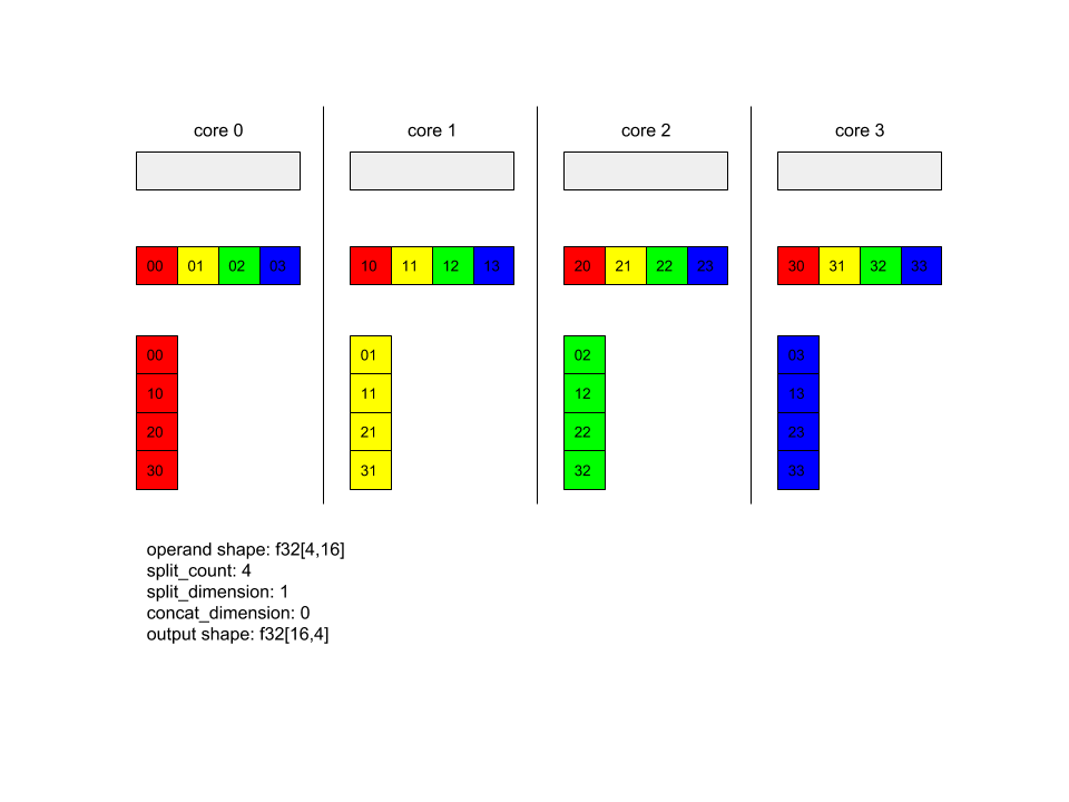
W tym przykładzie wszystkie 4 rdzenie są częścią zasobu Alltoall. W każdym rdzeń operand jest dzielony na 4 części wzdłuż wymiaru 0, więc każda z nich ma kształt f32[4,4]. Te 4 części są rozproszone po wszystkich rdzeniach. Następnie każdy rdzeń łączy otrzymane części wzdłuż wymiaru 1 w kolejności rdzeni 0–4. Dane wyjściowe na każdym rdzeń mają więc kształt f32[16,4].
BatchNormGrad
Szczegółowy opis algorytmu znajdziesz też w XlaBuilder::BatchNormGrad i pierwotnej dokumentacji do normalizacji grupowej.
Oblicza gradienty normy wsadowej.
BatchNormGrad(operand, scale, mean, variance, grad_output, epsilon, feature_index)
| Argumenty | Typ | Semantyka |
|---|---|---|
operand |
XlaOp |
n-wymiarowa tablica wymiarowa do znormalizowania (x) |
scale |
XlaOp |
1 tablica wymiarowa (\(\gamma\)) |
mean |
XlaOp |
1 tablica wymiarowa (\(\mu\)) |
variance |
XlaOp |
1 tablica wymiarowa (\(\sigma^2\)) |
grad_output |
XlaOp |
Gradienty przekazane do zakresu BatchNormTraining (\(\nabla y\)) |
epsilon |
float |
Wartość epsilonu (\(\epsilon\)) |
feature_index |
int64 |
Indeks do wymiaru cechy w: operand |
W przypadku każdej cechy w wymiarze cechy (feature_index to indeks wymiaru obiektu w argumencie operand) operacja oblicza gradienty z uwzględnieniem operand, offset i scale we wszystkich pozostałych wymiarach. Wartość feature_index musi być prawidłowym indeksem wymiaru cechy w tabeli operand.
Trzy gradienty są definiowane za pomocą tych formuł (przy założeniu, że czterowymiarowa tablica to operand, indeks wymiarów cech l, rozmiar wsadu m oraz rozmiary przestrzenne w i h):
\[ \begin{split} c_l&= \frac{1}{mwh}\sum_{i=1}^m\sum_{j=1}^w\sum_{k=1}^h \left( \nabla y_{ijkl} \frac{x_{ijkl} - \mu_l}{\sigma^2_l+\epsilon} \right) \\\\ d_l&= \frac{1}{mwh}\sum_{i=1}^m\sum_{j=1}^w\sum_{k=1}^h \nabla y_{ijkl} \\\\ \nabla x_{ijkl} &= \frac{\gamma_{l} }{\sqrt{\sigma^2_{l}+\epsilon} } \left( \nabla y_{ijkl} - d_l - c_l (x_{ijkl} - \mu_{l}) \right) \\\\ \nabla \gamma_l &= \sum_{i=1}^m\sum_{j=1}^w\sum_{k=1}^h \left( \nabla y_{ijkl} \frac{x_{ijkl} - \mu_l}{\sqrt{\sigma^2_{l}+\epsilon} } \right) \\\\\ \nabla \beta_l &= \sum_{i=1}^m\sum_{j=1}^w\sum_{k=1}^h \nabla y_{ijkl} \end{split} \]
Dane wejściowe mean i variance reprezentują wartości momentów w wymiarach wsadowych i przestrzennych.
Typ wyjściowy jest kropką złożoną z 3 nicków:
| Wyniki | Typ | Semantyka |
|---|---|---|
grad_operand
|
XlaOp
|
gradient względem danych wejściowych operand ($\nabla
x$) |
grad_scale
|
XlaOp
|
gradient względem danych wejściowych scale ($\nabla
\gamma$) |
grad_offset
|
XlaOp
|
gradient względem danych wejściowych offset($\nabla
\beta$) |
BatchNormInference
Szczegółowy opis algorytmu znajdziesz też w XlaBuilder::BatchNormInference i pierwotnej dokumentacji do normalizacji grupowej.
Normalizuje tablicę w wymiarach wsadowych i przestrzennych.
BatchNormInference(operand, scale, offset, mean, variance, epsilon, feature_index)
| Argumenty | Typ | Semantyka |
|---|---|---|
operand |
XlaOp |
n-wymiarowa tablica do znormalizowania |
scale |
XlaOp |
1 tablica wymiarowa |
offset |
XlaOp |
1 tablica wymiarowa |
mean |
XlaOp |
1 tablica wymiarowa |
variance |
XlaOp |
1 tablica wymiarowa |
epsilon |
float |
Wartość epsilonu |
feature_index |
int64 |
Indeks do wymiaru cechy w: operand |
W przypadku każdej cechy w wymiarze cech (feature_index to indeks wymiaru cechy w operand) operacja oblicza średnią i wariancję we wszystkich pozostałych wymiarach, a potem wykorzystuje średnią i wariancję do normalizacji każdego elementu w wymiarze operand. Wartość feature_index musi być prawidłowym indeksem wymiaru cechy w tabeli operand.
Funkcja BatchNormInference jest odpowiednikiem wywoływania funkcji BatchNormTraining bez obliczania poszczególnych operacji wsadowych mean i variance. Używa wtedy danych wejściowych mean i variance jako wartości szacunkowych. Ta operacja ma na celu zmniejszenie opóźnienia wnioskowania, stąd nazwa BatchNormInference.
Wynikiem jest n-wymiarowa, znormalizowana tablica o tym samym kształcie co wejściowa operand.
BatchNormTraining
Szczegółowy opis algorytmu znajdziesz też w sekcjach XlaBuilder::BatchNormTraining i the original batch normalization paper.
Normalizuje tablicę w wymiarach wsadowych i przestrzennych.
BatchNormTraining(operand, scale, offset, epsilon, feature_index)
| Argumenty | Typ | Semantyka |
|---|---|---|
operand |
XlaOp |
n-wymiarowa tablica wymiarowa do znormalizowania (x) |
scale |
XlaOp |
1 tablica wymiarowa (\(\gamma\)) |
offset |
XlaOp |
1 tablica wymiarowa (\(\beta\)) |
epsilon |
float |
Wartość epsilonu (\(\epsilon\)) |
feature_index |
int64 |
Indeks do wymiaru cechy w: operand |
W przypadku każdej cechy w wymiarze cech (feature_index to indeks wymiaru cechy w operand) operacja oblicza średnią i wariancję we wszystkich pozostałych wymiarach, a potem wykorzystuje średnią i wariancję do normalizacji każdego elementu w wymiarze operand. Wartość feature_index musi być prawidłowym indeksem wymiaru cechy w tabeli operand.
Algorytm działa w ten sposób w przypadku każdej wsadu w pliku operand \(x\) , który zawiera elementy m z rozmiarami w i h jako wymiarami przestrzennymi (przy założeniu, że operand to tablica czterowymiarowa):
Oblicza średnią zbiorczą \(\mu_l\) dla każdej cechy
lw wymiarze cech:\(\mu_l=\frac{1}{mwh}\sum_{i=1}^m\sum_{j=1}^w\sum_{k=1}^h x_{ijkl}\)Oblicza wariancję wsadową \(\sigma^2_l\): $\sigma^2l=\frac{1}{mwh}\sum{i=1}^m\sum{j=1}^w\sum{k=1}^h (x_{ijkl} - \mu_l)^2$
Normalizacja, skalowanie i przesunięcie: \(y_{ijkl}=\frac{\gamma_l(x_{ijkl}-\mu_l)}{\sqrt[2]{\sigma^2_l+\epsilon} }+\beta_l\)
Wartość epsilonu, zwykle mała liczba, jest dodawana, aby uniknąć błędów dzielenia przez 0.
Typ wyjściowy jest kropką 3 elementów XlaOp:
| Wyniki | Typ | Semantyka |
|---|---|---|
output
|
XlaOp
|
n-wymiarowa tablica wymiarowa o takim samym kształcie co w przypadku danych wejściowych operand (y) |
batch_mean |
XlaOp |
1 tablica wymiarowa (\(\mu\)) |
batch_var |
XlaOp |
1 tablica wymiarowa (\(\sigma^2\)) |
Wartości batch_mean i batch_var to momenty obliczone w wymiarach wsadowych i przestrzennych za pomocą powyższych wzorów.
BitcastConvertType
Zobacz też XlaBuilder::BitcastConvertType.
Podobnie jak tf.bitcast w TensorFlow, wykonuje operację bitcastu z wykorzystaniem kształtu danych na obiekt docelowy. Rozmiar danych wejściowych i wyjściowych musi być taki sam, np. elementy s32 stają się elementami f32 za pomocą procedury bitcastu, a 1 element s32 stanie się 4 elementami s8. Bitcast jest implementowany jako rzut niskopoziomowy, dlatego maszyny z różnymi reprezentacjami zmiennoprzecinkowymi dostaną różne wyniki.
BitcastConvertType(operand, new_element_type)
| Argumenty | Typ | Semantyka |
|---|---|---|
operand |
XlaOp |
tablica typu T z przyciemnieniem D |
new_element_type |
PrimitiveType |
typ U |
Wymiary operandu i docelowego kształtu muszą być takie same. Wyjątkiem jest ostatni wymiar, który będzie się zmieniał odpowiednio do współczynnika rozmiaru podstawowego przed konwersją i po niej.
Typymi elementów źródłowych i docelowych nie mogą być krotki.
Konwersja bitcasta na typ podstawowy o różnej szerokości
Instrukcja BitcastConvert HLO obsługuje przypadek, w którym rozmiar elementu wyjściowego typu T' nie jest równy rozmiarowi elementu wejściowego T. Ponieważ cała operacja jest koncepcyjnie metodą bitcastu i nie zmienia podstawowych bajtów, kształt elementu wyjściowego musi się zmienić. W przypadku właściwości B = sizeof(T), B' =
sizeof(T') możliwe są 2 przypadki.
Po pierwsze, gdy B > B' kształt wyjściowy otrzymuje nowy, mniejszy wymiar rozmiaru
B/B'. Na przykład:
f16[10,2]{1,0} %output = f16[10,2]{1,0} bitcast-convert(f32[10]{0} %input)
W przypadku skutecznych skalarów reguła pozostaje taka sama:
f16[2]{0} %output = f16[2]{0} bitcast-convert(f32[] %input)
Z kolei w przypadku parametru B' > B instrukcja wymaga, aby ostatni wymiar logiczny wejściowego kształtu był równy B'/B. Ten wymiar jest pomijany podczas konwersji:
f32[10]{0} %output = f32[10]{0} bitcast-convert(f16[10,2]{1,0} %input)
Pamiętaj, że konwersje między różnymi szerokościami transmisji nie są uwzględniane w przypadku elementów.
Komunikaty
Zobacz też XlaBuilder::Broadcast.
Dodaje wymiary do tablicy przez zduplikowanie w niej danych.
Broadcast(operand, broadcast_sizes)
| Argumenty | Typ | Semantyka |
|---|---|---|
operand |
XlaOp |
Tablica do duplikowania |
broadcast_sizes |
ArraySlice<int64> |
Rozmiary nowych wymiarów |
Nowe wymiary zostaną wstawione po lewej stronie, np. jeśli broadcast_sizes ma wartości {a0, ..., aN}, a kształt argumentu ma wymiary {b0, ..., bM}, kształt wyniku ma wymiary {a0, ..., aN, b0, ..., bM}.
Nowe wymiary są indeksowane do kopii operandu, tj.
output[i0, ..., iN, j0, ..., jM] = operand[j0, ..., jM]
Jeśli na przykład operand jest skalarnym f32 o wartości 2.0f, a broadcast_sizes to {2, 3}, wynikiem będzie tablica o kształcie f32[2, 3], a wszystkie wartości w wyniku będą wynosić 2.0f.
BroadcastInDim
Zobacz też XlaBuilder::BroadcastInDim.
Rozszerza rozmiar i pozycję tablicy przez zduplikowanie zawartych w niej danych.
BroadcastInDim(operand, out_dim_size, broadcast_dimensions)
| Argumenty | Typ | Semantyka |
|---|---|---|
operand |
XlaOp |
Tablica do duplikowania |
out_dim_size |
ArraySlice<int64> |
rozmiary wymiarów docelowego kształtu; |
broadcast_dimensions |
ArraySlice<int64> |
Którego wymiaru w kształcie docelowym odpowiada każdy wymiar kształtu argumentu |
Podobnie jak w przypadku transmisji, ale umożliwia dodawanie wymiarów w dowolnym miejscu i rozwijanie istniejących wymiarów o rozmiar 1.
Wartość operand jest przekazywana do kształtu opisanego przez out_dim_size.
Funkcja broadcast_dimensions mapuje wymiary elementu operand na wymiary docelowego kształtu, tzn. i-ty wymiar operandu jest mapowany na wymiar kształtu wyjściowego. Wymiary obiektu operand muszą mieć rozmiar 1 lub być takie same jak wymiar w kształcie wyjściowym, na który są zmapowane. Pozostałe wymiary są wypełniane wymiarami rozmiaru 1. Transmisja o zdegenerowanych wymiarach jest przesyłana wzdłuż tych degenerowanych wymiarów, aby dotrzeć do kształtu wyjściowego. Semantyka jest szczegółowo opisana na stronie transmisji.
Połączenie
Zobacz też XlaBuilder::Call.
Wywołuje obliczenia przy użyciu podanych argumentów.
Call(computation, args...)
| Argumenty | Typ | Semantyka |
|---|---|---|
computation |
XlaComputation |
obliczenia typu T_0, T_1, ..., T_{N-1} -> S z N parametrami dowolnego typu |
args |
sekwencja N XlaOp s |
N argumentów dowolnego typu |
arity i typy obiektu args muszą być zgodne z parametrami właściwości computation. Nie może zawierać żadnych elementów typu args.
Choleski
Zobacz też XlaBuilder::Cholesky.
Oblicza rozkład Cholesky'ego w grupie macierzystych symetrycznych (hermickich) dodatnich.
Cholesky(a, lower)
| Argumenty | Typ | Semantyka |
|---|---|---|
a |
XlaOp |
macierz > 2 typu zespolonego lub zmiennoprzecinkowego. |
lower |
bool |
określa, czy użyć górnego, czy dolnego trójkąta a. |
Jeśli lower to true, oblicza macierze dolnych trójkątów l w taki sposób, że $a = l .
l^T$. Jeśli lower ma wartość false, oblicza macierze górne trójkątów u w taki sposób, aby:\(a = u^T . u\).
Dane wejściowe są odczytywane tylko z górnego/dolnego trójkąta a (w zależności od wartości lower). Wartości z drugiego trójkąta są ignorowane. Dane wyjściowe są zwracane w tym samym trójkącie. Wartości w drugim trójkącie są zdefiniowane przez implementację i mogą być dowolne.
Jeśli pozycja a jest większa niż 2, a jest traktowana jako grupa macierzy, gdzie wszystkie oprócz 2 podrzędnych wymiarów są wymiarami wsadowymi.
Jeśli funkcja a nie jest symetryczna (hermita) określona jako dodatnia, wynik jest definiowany przez implementację.
Z klipsem
Zobacz też XlaBuilder::Clamp.
Łączy operand w zakresie między wartością minimalną a maksymalną.
Clamp(min, operand, max)
| Argumenty | Typ | Semantyka |
|---|---|---|
min |
XlaOp |
tablica typu T |
operand |
XlaOp |
tablica typu T |
max |
XlaOp |
tablica typu T |
Biorąc pod uwagę operand oraz wartości minimalną i maksymalną, zwraca operand, jeśli mieści się on w zakresie między wartością minimalną a maksymalną. W przeciwnym razie zwraca wartość minimalną, jeśli operand jest poniżej tego zakresu, lub wartość maksymalną, jeśli operand jest powyżej tego zakresu. Czyli clamp(a, x, b) = min(max(a, x), b).
Wszystkie trzy tablice muszą mieć ten sam kształt. W ramach ograniczonej formy transmisji min lub max mogą być skalarem typu T.
Przykład ze skalarnymi min i max:
let operand: s32[3] = {-1, 5, 9};
let min: s32 = 0;
let max: s32 = 6;
==>
Clamp(min, operand, max) = s32[3]{0, 5, 6};
Zwiń
Zobacz też XlaBuilder::Collapse i operację tf.reshape.
Zwija wymiary tablicy do jednego wymiaru.
Collapse(operand, dimensions)
| Argumenty | Typ | Semantyka |
|---|---|---|
operand |
XlaOp |
tablica typu T |
dimensions |
Wektor int64 |
w kolejności, następujących po sobie podzbiorów wymiarów T. |
Opcja Zwiń zastępuje dany podzbiór wymiarów argumentu jednym wymiarem. Argumenty wejściowe to dowolna tablica typu T i wektor stałej kompilacji w indeksach wymiarów. Indeksy wymiarów muszą być ułożone w kolejności (od najmniejszej do największej wartości), będącej następującym podzbiorem wymiarów T. W związku z tym wszystkie wartości {0, 1, 2}, {0, 1} i {1, 2} są prawidłowymi zestawami wymiarów, ale {1, 0} ani {0, 2} już nie. Są one zastępowane jednym nowym wymiarem o tej samej pozycji w sekwencji wymiarów co te, które zastępują, nowym rozmiarem równym iloczynowi rozmiarów pierwotnych wymiarów. Najniższa liczba wymiarów w polu dimensions to najwolniejszy wymiar (największy) w zagnieżdżeniu pętli, który zwija te wymiary. Najwyższa liczba wymiarów zmienia się najszybciej (w większości mniejszych). Jeśli potrzebujesz bardziej ogólnej kolejności zwijania, zapoznaj się z operatorem tf.reshape.
Na przykład niech v będzie tablicą 24 elementów:
let v = f32[4x2x3] { { {10, 11, 12},  {15, 16, 17} },
{ {20, 21, 22},  {25, 26, 27} },
{ {30, 31, 32},  {35, 36, 37} },
{ {40, 41, 42},  {45, 46, 47} } };

// Collapse to a single dimension, leaving one dimension.
let v012 = Collapse(v, {0,1,2});
then v012 == f32[24] {10, 11, 12, 15, 16, 17,
20, 21, 22, 25, 26, 27,
30, 31, 32, 35, 36, 37,
40, 41, 42, 45, 46, 47};

// Collapse the two lower dimensions, leaving two dimensions.
let v01 = Collapse(v, {0,1});
then v01 == f32[4x6] { {10, 11, 12, 15, 16, 17},
{20, 21, 22, 25, 26, 27},
{30, 31, 32, 35, 36, 37},
{40, 41, 42, 45, 46, 47} };

// Collapse the two higher dimensions, leaving two dimensions.
let v12 = Collapse(v, {1,2});
then v12 == f32[8x3] { {10, 11, 12},
{15, 16, 17},
{20, 21, 22},
{25, 26, 27},
{30, 31, 32},
{35, 36, 37},
{40, 41, 42},
{45, 46, 47} };
CollectivePermute
Zobacz też XlaBuilder::CollectivePermute.
CollectivePermute to zbiorcza operacja, która wysyła i odbiera krzyżowe repliki danych.
CollectivePermute(operand, source_target_pairs)
| Argumenty | Typ | Semantyka |
|---|---|---|
operand |
XlaOp |
n-wymiarowa tablica wejściowa |
source_target_pairs |
Wektor <int64, int64> |
Lista par (source_replica_id, target_replica_id). Dla każdej pary operand jest wysyłany z repliki źródłowej do docelowej repliki. |
Pamiętaj, że source_target_pair ma następujące ograniczenia:
- Dowolne 2 pary nie powinny mieć tego samego identyfikatora repliki docelowej ani nie powinny mieć tego samego identyfikatora repliki źródłowej.
- Jeśli identyfikator repliki nie jest celem w żadnej parze, dane wyjściowe tej repliki to tensor składający się z 0 o tym samym kształcie co dane wejściowe.
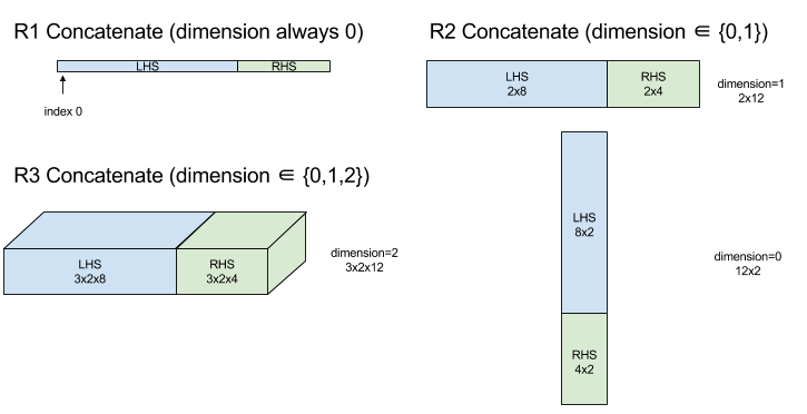
Połącz
Zobacz też XlaBuilder::ConcatInDim.
Konkatenacja tworzy tablicę z wielu argumentów tablicy. Tablica ma tę samą pozycję co każdy operand tablicy wejściowej (musi mieć tę samą pozycję co pozostałe) i zawiera argumenty w kolejności, w jakiej zostały określone.
Concatenate(operands..., dimension)
| Argumenty | Typ | Semantyka |
|---|---|---|
operands |
sekwencja N XlaOp |
Tablice N typu T o wymiarach [L0, L1, ...]. Wymagane: N >= 1. |
dimension |
int64 |
Wartość z przedziału [0, N) określająca wymiar do połączenia między elementami operands. |
Wszystkie wymiary z wyjątkiem dimension muszą być takie same. Dzieje się tak, ponieważ XLA nie obsługuje „przeszklonych” tablic. Pamiętaj też, że wartości rankingu 0 nie mogą być łączone (ponieważ nie można nazwać wymiaru, według którego następuje łączenie).
Przykład jednowymiarowy:
Concat({ {2, 3}, {4, 5}, {6, 7} }, 0)
>>> {2, 3, 4, 5, 6, 7}
Przykład obrazu dwuwymiarowego:
let a = {
{1, 2},
{3, 4},
{5, 6},
};
let b = {
{7, 8},
};
Concat({a, b}, 0)
>>> {
{1, 2},
{3, 4},
{5, 6},
{7, 8},
}
Diagram:
Warunkowy
Zobacz też XlaBuilder::Conditional.
Conditional(pred, true_operand, true_computation, false_operand,
false_computation)
| Argumenty | Typ | Semantyka |
|---|---|---|
pred |
XlaOp |
Skalar typu PRED |
true_operand |
XlaOp |
Argument typu \(T_0\) |
true_computation |
XlaComputation |
XlaComputation typu \(T_0 \to S\) |
false_operand |
XlaOp |
Argument typu \(T_1\) |
false_computation |
XlaComputation |
XlaComputation typu \(T_1 \to S\) |
Wykonuje polecenie true_computation, jeśli pred ma wartość true, false_computation, jeśli pred to false, i zwraca wynik.
true_computation musi przyjmować pojedynczy argument typu \(T_0\) i będzie wywoływany z true_operand, który musi być tego samego typu. false_computation musi przyjmować pojedynczy argument typu \(T_1\) i jest wywoływany z false_operand, który musi być tego samego typu. Typ zwróconej wartości true_computation i false_computation musi być taki sam.
Pamiętaj, że w zależności od wartości pred zostanie wykonane tylko jedno z tych działań: true_computation i false_computation.
Conditional(branch_index, branch_computations, branch_operands)
| Argumenty | Typ | Semantyka |
|---|---|---|
branch_index |
XlaOp |
Skalar typu S32 |
branch_computations |
sekwencja N XlaComputation |
XlaComputations typu \(T_0 \to S , T_1 \to S , ..., T_{N-1} \to S\) |
branch_operands |
sekwencja N XlaOp |
Argumenty typu \(T_0 , T_1 , ..., T_{N-1}\) |
Wykonuje polecenie branch_computations[branch_index] i zwraca wynik. Jeśli branch_index to S32, który ma wartość < 0 lub >= N, jako gałąź domyślna wykonywana jest branch_computations[N-1].
Każdy element branch_computations[b] musi przyjąć 1 argument typu \(T_b\) i będzie wywoływany z funkcją branch_operands[b], która musi być tego samego typu. Typ zwracanej wartości każdego elementu branch_computations[b] musi być taki sam.
Pamiętaj, że w zależności od wartości branch_index zostanie wykonany tylko 1 z zastosowań polecenia branch_computations.
Konw (konwersja)
Zobacz też XlaBuilder::Conv.
Jako ConvWithGeneralPadding, ale dopełnienie jest określane w skrócie jako SAME lub Prawidłowe. SAME dopełnienie wypełnia dane wejściowe (lhs) zerami, dzięki czemu dane wyjściowe mają taki sam kształt jak dane wejściowe, jeśli nie są brane pod uwagę. Prawidłowe dopełnienie oznacza po prostu brak dopełnienia.
ConvWithGeneralPadding (konwolucja)
Zobacz też XlaBuilder::ConvWithGeneralPadding.
Oblicza splot takiego typu jak w sieciach neuronowych. W tym przypadku splot można uznać za okno n-wymiarowe poruszające się po n-wymiarowym obszarze podstawy, a obliczenia są wykonywane dla każdej możliwej pozycji okna.
| Argumenty | Typ | Semantyka |
|---|---|---|
lhs |
XlaOp |
tablica wejściowa typu n+2 |
rhs |
XlaOp |
tablica n+2 wag jądra systemu |
window_strides |
ArraySlice<int64> |
Tablica n-d kroków jądra |
padding |
ArraySlice< pair<int64,int64>> |
Tablica n-d z dopełnieniem (niskie, wysokie) |
lhs_dilation |
ArraySlice<int64> |
Tablica współczynnika dylatacji n-d lhs |
rhs_dilation |
ArraySlice<int64> |
Tablica współczynnika dylatacji n-d rhs |
feature_group_count |
int64 | liczbę grup cech |
batch_group_count |
int64 | liczbę grup wsadowych; |
Niech będzie liczbą wymiarów przestrzennych n. Argument lhs to tablica n+2 opisująca pole bazowe. Nazywamy to danymi wejściowymi, chociaż rhs też jest wartością wejściową. W sieci neuronowej są to aktywacje wejściowe.
Wymiary n+2 są podane w tej kolejności:
batch: każda współrzędna w tym wymiarze stanowi niezależne dane wejściowe, dla których przeprowadzany jest splot.z/depth/features: z każdą pozycją (y,x) w obszarze podstawowym jest powiązany z nią wektor, który określa ten wymiar.spatial_dims: opisuje wymiary przestrzennenokreślające obszar podstawowy, po którym porusza się okno.
Argument rhs to tablica n+2 opisująca filtr splotowy/jądro/okno. Wymiary są podane w tej kolejności:
output-z: wymiarzdanych wyjściowych.input-z: rozmiar tego wymiaru pomnożony przezfeature_group_countpowinien być równy rozmiarowi wymiaruzw lh.spatial_dims: opisuje wymiary przestrzennen, które definiują okno n-d – poruszające się po obszarze bazowym.
Argument window_strides określa krok okna splotowego w wymiarach przestrzennych. Jeśli np. krok w pierwszym wymiarze przestrzennym wynosi 3, okno można umieścić tylko we współrzędnych, w których pierwszy indeks przestrzenny jest podzielony przez 3.
Argument padding określa wartość zero dopełnienia, które ma zostać zastosowane do obszaru podstawowego. Ilość dopełnienia może być ujemna – bezwzględna wartość dopełnienia ujemnego wskazuje liczbę elementów, które należy usunąć z określonego wymiaru przed wykonaniem splotu. padding[0] określa dopełnienie wymiaru y, a padding[1] – dopełnienie wymiaru x. Każda para ma niskie dopełnienie jako pierwszy element, a wysokie dopełnienie jako drugi element. Małe dopełnienie jest stosowane w kierunku dolnych indeksów, a duże w kierunku wyższych indeksów. Jeśli np. padding[1] ma wartość (2,3), w drugim wymiarze przestrzennym po lewej stronie pojawi się dopełnienie o 2 zera po lewej stronie i 3 zera po prawej stronie. Użycie dopełnienia jest równoważne wstawieniu do danych wejściowych (lhs) tych samych wartości zerowych przed wykonaniem splotu.
Argumenty lhs_dilation i rhs_dilation określają współczynnik dylatacji, który jest stosowany odpowiednio do pól lhs i rh w każdym wymiarze przestrzennym. Jeśli współczynnik poszerzenia w wymiarze przestrzennym wynosi d, otwory d-1 są domyślnie umieszczane między poszczególnymi elementami w tym wymiarze, co zwiększa rozmiar tablicy. Otwory są wypełniane wartością „no-op”, co dla splotu oznacza zero.
Rozszerzenie Rhs jest też nazywane splotem zaburzeń. Więcej informacji: tf.nn.atrous_conv2d. Rozszerzenie kanału jest też nazywane splotem transponowanym. Więcej informacji: tf.nn.conv2d_transpose.
Argumentu feature_group_count (wartość domyślna 1) można używać do zgrupowanych splotów. feature_group_count musi być dzielnikiem zarówno danych wejściowych, jak i wyjściowych. Jeśli feature_group_count ma wartość większą niż 1, oznacza to, że koncepcyjnie wymiar cech wejściowych i wyjściowych oraz wymiar cech wyjściowych rhs są dzielone po równo na wiele grup feature_group_count, z których każda składa się z kolejnej części cech. Wymiar cechy wejściowej rhs musi być równy wymiarowi cechy wejściowej lhs podzielonej przez feature_group_count (tak aby miał już rozmiar grupy cech wejściowych). Grupy i-te są używane razem do obliczania feature_group_count dla wielu oddzielnych splotów. Wyniki tych splotów są łączone w wymiarze cech wyjściowych.
W przypadku splotu głębiej argument feature_group_count zostałby ustawiony na wymiar cechy wejściowej, a kształt filtra zmieniłby się z [filter_height, filter_width, in_channels, channel_multiplier] na [filter_height, filter_width, 1, in_channels * channel_multiplier]. Więcej informacji: tf.nn.depthwise_conv2d.
Argumentu batch_group_count (wartość domyślna 1) można używać do zgrupowanych filtrów podczas rozpowszechniania wstecznego. batch_group_count musi być dzielnikiem rozmiaru wsadu lhs (wejściowej). Jeśli batch_group_count ma wartość większą niż 1, oznacza to, że rozmiar wyjściowego wsadu powinien mieć rozmiar input batch
/ batch_group_count. Element batch_group_count musi być dzielnikiem rozmiaru cechy wyjściowej.
Kształt wyjściowy ma następujące wymiary w tej kolejności:
batch: rozmiar tego wymiaru pomnożony przezbatch_group_countpowinien być równy rozmiarowi wymiarubatchw plikach danych.z: taki sam rozmiar jak w przypadku plikuoutput-zw jądrze (rhs).spatial_dims: po 1 wartości na każde prawidłowe położenie okna konwolucyjnego.

Na ilustracji powyżej widać, jak działa pole batch_group_count. W efekcie dzielimy każdy wsad plików SDF na grupy batch_group_count i to samo robimy w przypadku cech wyjściowych. Następnie w przypadku każdej z tych grup tworzymy sploty w parach i łączymy dane wyjściowe w wymiarze cechy wyjściowej. Semantyka operacyjna wszystkich innych wymiarów (cecha i przestrzenna) pozostaje taka sama.
Prawidłowe położenie okna splotowego zależą od liczby kroków i rozmiaru obszaru podstawowego po dopełnieniu.
Aby opisać działanie splotu, rozważ splot 2D i wybierz stałe współrzędne batch, z, y i x w wyniku. (y,x) to pozycja rogu okna w obszarze podstawy (np. lewy górny róg okna w zależności od interpretacji wymiarów przestrzennych). Mamy teraz okno 2d
pobrane z obszaru podstawowego, gdzie każdy punkt 2d jest powiązany z wektorem 1d, w ten sposób otrzymujemy ramkę 3d. Po ustaleniu współrzędnej wyjściowej z w jądrze splotowym mamy też szafkę 3D. Oba pola mają te same wymiary, więc możemy obliczyć sumę iloczynów elementów z obu pól (podobnie do iloczynu skalarnego). Jest to wartość wyjściowa.
Pamiętaj, że jeśli output-z to np. 5, każda pozycja okna daje w danych wyjściowych 5 wartości w wymiarze z danych wyjściowych. Wartości te różnią się tym, która część jądra splotowego została wykorzystana – każda współrzędna output-z ma osobne pole 3D z wartościami. Wyobraź sobie 5 osobnych splotów
i każdy z nich ma inny filtr.
Oto pseudokod 2D splotu z dopełnieniem i krokiem:
for (b, oz, oy, ox) {  // output coordinates
  value = 0;
  for (iz, ky, kx) {  // kernel coordinates and input z
    iy = oy*stride_y + ky - pad_low_y;
    ix = ox*stride_x + kx - pad_low_x;
    if ((iy, ix) inside the base area considered without padding) {
      value += input(b, iz, iy, ix) * kernel(oz, iz, ky, kx);
    }
  }
  output(b, oz, oy, ox) = value;
}
ConvertElementType
Zobacz też XlaBuilder::ConvertElementType.
Podobnie jak static_cast w przypadku elementów w języku C++, wykonuje operację konwersji na poziomie elementu z kształtu danych na docelowy. Wymiary muszą być takie same, a konwersja następuje na podstawie poszczególnych elementów, np. w ramach procedury konwersji s32-f32 elementy s32 zmieniają się w elementy f32.
ConvertElementType(operand, new_element_type)
| Argumenty | Typ | Semantyka |
|---|---|---|
operand |
XlaOp |
tablica typu T z przyciemnieniem D |
new_element_type |
PrimitiveType |
typ U |
Wymiary operandu i docelowego kształtu muszą być takie same. Typymi elementów źródłowych i docelowych nie mogą być krotki.
Konwersja, np. z T=s32 na U=f32, wykona procedurę normalizacji liczby zmiennoprzecinkowej, np. zaokrąglenia do najmniejszej równomierności.
let a: s32[3] = {0, 1, 2};
let b: f32[3] = convert(a, f32);
then b == f32[3]{0.0, 1.0, 2.0}
CrossReplicaSum
Wykonuje obliczenia AllReduce przy użyciu obliczania sumy.
CustomCall
Zobacz też XlaBuilder::CustomCall.
Wywoływanie w ramach obliczeń funkcji udostępnionej przez użytkownika.
CustomCall(target_name, args..., shape)
| Argumenty | Typ | Semantyka |
|---|---|---|
target_name |
string |
Nazwa funkcji. Zostanie wysłana instrukcja rozmowy kierowana na tę nazwę symbolu. |
args |
sekwencja N XlaOp s |
N argumentów dowolnego typu, które zostaną przekazane do funkcji. |
shape |
Shape |
Kształt wyjściowy funkcji |
Podpis funkcji jest taki sam niezależnie od istotności i typu argumentów:
extern "C" void target_name(void* out, void** in);
Jeśli funkcja CustomCall jest używana na przykład w następujący sposób:
let x = f32[2] {1,2};
let y = f32[2x3] { {10, 20, 30}, {40, 50, 60} };

CustomCall("myfunc", {x, y}, f32[3x3])
Oto przykład implementacji myfunc:
extern "C" void myfunc(void* out, void** in) {
  float (&x)[2] = *static_cast<float(*)[2]>(in[0]);
  float (&y)[2][3] = *static_cast<float(*)[2][3]>(in[1]);
  EXPECT_EQ(1, x[0]);
  EXPECT_EQ(2, x[1]);
  EXPECT_EQ(10, y[0][0]);
  EXPECT_EQ(20, y[0][1]);
  EXPECT_EQ(30, y[0][2]);
  EXPECT_EQ(40, y[1][0]);
  EXPECT_EQ(50, y[1][1]);
  EXPECT_EQ(60, y[1][2]);
  float (&z)[3][3] = *static_cast<float(*)[3][3]>(out);
  z[0][0] = x[1] + y[1][0];
  // ...
}
Funkcja podana przez użytkownika nie może mieć skutków ubocznych, a jej wykonanie musi być identyczne.
Kropka
Zobacz też XlaBuilder::Dot.
Dot(lhs, rhs)
| Argumenty | Typ | Semantyka |
|---|---|---|
lhs |
XlaOp |
tablica typu T |
rhs |
XlaOp |
tablica typu T |
Dokładna semantyka tej operacji zależy od pozycji operandów:
| Dane wejściowe | Wyniki | Semantyka |
|---|---|---|
wektor [n] wektor dot [n] |
wartość skalarna | iloczyn skalarny wektorowy |
macierz [m x k] wektor dot [k] |
wektor [m] | mnożenie wektorów macierzy |
macierz [m x k] dot macierz [k x n] |
macierz [m x n] | mnożenie macierzy |
Operacja wykonuje sumę produktów w drugim wymiarze, czyli lhs (lub pierwszym, jeśli ma pozycję 1) i w pierwszym wymiarze – rhs. Są to wymiary „skrócone”. Zakontraktowane wymiary elementów lhs i rhs muszą być tego samego rozmiaru. W praktyce można go używać do wykonywania iloczynów skalarnych między wektorami, mnożenia wektorów/macierz lub macierzy.
DotGeneral
Zobacz też XlaBuilder::DotGeneral.
DotGeneral(lhs, rhs, dimension_numbers)
| Argumenty | Typ | Semantyka |
|---|---|---|
lhs |
XlaOp |
tablica typu T |
rhs |
XlaOp |
tablica typu T |
dimension_numbers |
DotDimensionNumbers |
numery umów i wymiarów wsadowych |
Działa podobnie jak kropka, ale umożliwia podawanie numerów wymiarów objętych umową i wymiarów wsadowych zarówno w przypadku lhs, jak i rhs.
| Pola DotDimensionsNumbers | Typ | Semantyka |
|---|---|---|
lhs_contracting_dimensions
|
powtórzony int64 | lhs numeru wymiaru umowy |
rhs_contracting_dimensions
|
powtórzony int64 | rhs numeru wymiaru umowy |
lhs_batch_dimensions
|
powtórzony int64 | lhs numerów wymiarów wsadowych |
rhs_batch_dimensions
|
powtórzony int64 | rhs numerów wymiarów wsadowych |
DotGeneral sprawdza sumę produktów w wymiarach związanych z umową, które są określone we właściwości dimension_numbers.
Powiązane numery wymiarów objętych umową lhs i rhs nie muszą być takie same, ale muszą mieć te same rozmiary wymiarów.
Przykład z numerami wymiarów objętych umową:
lhs = { {1.0, 2.0, 3.0},
{4.0, 5.0, 6.0} }

rhs = { {1.0, 1.0, 1.0},
{2.0, 2.0, 2.0} }

DotDimensionNumbers dnums;
dnums.add_lhs_contracting_dimensions(1);
dnums.add_rhs_contracting_dimensions(1);

DotGeneral(lhs, rhs, dnums) -> { {6.0, 12.0},
{15.0, 30.0} }
Powiązane numery wymiarów w tabelach lhs i rhs muszą mieć te same rozmiary.
Przykład z numerami wymiarów wsadu (matryca wsadu 2, matryce 2 x 2):
lhs = { { {1.0, 2.0},
{3.0, 4.0} },
{ {5.0, 6.0},
{7.0, 8.0} } }

rhs = { { {1.0, 0.0},
{0.0, 1.0} },
{ {1.0, 0.0},
{0.0, 1.0} } }

DotDimensionNumbers dnums;
dnums.add_lhs_contracting_dimensions(2);
dnums.add_rhs_contracting_dimensions(1);
dnums.add_lhs_batch_dimensions(0);
dnums.add_rhs_batch_dimensions(0);

DotGeneral(lhs, rhs, dnums) -> { { {1.0, 2.0},
{3.0, 4.0} },
{ {5.0, 6.0},
{7.0, 8.0} } }
| Dane wejściowe | Wyniki | Semantyka |
|---|---|---|
[b0, m, k] dot [b0, k, n] |
[b0, m, n] | wsad matmul |
[b0, b1, m, k] dot [b0, b1, k, n] |
[b0, b1, m, n] | wsad matmul |
Wynikowy numer wymiaru to zaczyna się od wymiaru wsadowego, następnie wymiaru lhs nieskróconego/niezbiorczego, a na końcu wymiaru rhs nieskurczącego/niezbiorczego.
DynamicSlice
Zobacz też XlaBuilder::DynamicSlice.
DynamicSlice wyodrębnia tablicę podrzędną z tablicy wejściowej w dynamicznej start_indices. Rozmiar wycinka w każdym wymiarze jest przekazywany w parametrze size_indices, który określa punkt końcowy wyłącznych przedziałów wycinków w poszczególnych wymiarach: [początek, początek + rozmiar). Kształt elementu start_indices musi mieć pozycję ==1, a rozmiar wymiaru równy pozycji operand.
DynamicSlice(operand, start_indices, size_indices)
| Argumenty | Typ | Semantyka |
|---|---|---|
operand |
XlaOp |
N tablica wymiarowa typu T |
start_indices |
sekwencja N XlaOp |
Lista N skalarnych liczb całkowitych zawierających początkowe indeksy wycinka dla każdego wymiaru. Wartość nie może być mniejsza niż 0. |
size_indices |
ArraySlice<int64> |
Lista N liczb całkowitych zawierających rozmiar wycinka każdego wymiaru. Każda wartość musi być większa niż 0, a wartość początkowa i rozmiar musi być mniejsza od rozmiaru wymiaru lub jej równa, aby uniknąć zawijania rozmiaru wymiaru modułu. |
Efektywne indeksy wycinków są obliczane przez zastosowanie tej przekształcenia do każdego indeksu i w [1, N) przed wykonaniem wycinka:
start_indices[i] = clamp(start_indices[i], 0, operand.dimension_size[i] - size_indices[i])
Dzięki temu wyodrębniony wycinek będzie zawsze w granicach względem tablicy argumentów. Jeśli przed zastosowaniem przekształcenia wycinek mieści się w jego granicach, przekształcenie nie przyniesie żadnego efektu.
Przykład jednowymiarowy:
let a = {0.0, 1.0, 2.0, 3.0, 4.0}
let s = {2}

DynamicSlice(a, s, {2}) produces:
{2.0, 3.0}
Przykład obrazu dwuwymiarowego:
let b =
{ {0.0,  1.0,  2.0},
{3.0,  4.0,  5.0},
{6.0,  7.0,  8.0},
{9.0, 10.0, 11.0} }
let s = {2, 1}

DynamicSlice(b, s, {2, 2}) produces:
{ { 7.0,  8.0},
{10.0, 11.0} }
DynamicUpdateSlice
Zobacz też XlaBuilder::DynamicUpdateSlice.
DynamicUpdateSlice generuje wynik będący wartością tablicy wejściowej operand, z wycinkiem update zastąpionym start_indices
Kształt tablicy update określa kształt tablicy podrzędnej wyniku, który jest aktualizowany.
Kształt elementu start_indices musi mieć pozycję == 1, a rozmiar wymiaru równy pozycji operand.
DynamicUpdateSlice(operand, update, start_indices)
| Argumenty | Typ | Semantyka |
|---|---|---|
operand |
XlaOp |
N tablica wymiarowa typu T |
update |
XlaOp |
N tablica wymiarowa typu T zawierająca aktualizację wycinka. Każdy wymiar kształtu aktualizacji musi być większy niż zero, a wartość początkowa i aktualizacja musi być mniejsza od lub równa rozmiar operandu każdego wymiaru, aby uniknąć generowania indeksów aktualizacji spoza granic. |
start_indices |
sekwencja N XlaOp |
Lista N skalarnych liczb całkowitych zawierających początkowe indeksy wycinka dla każdego wymiaru. Wartość nie może być mniejsza niż 0. |
Efektywne indeksy wycinków są obliczane przez zastosowanie tej przekształcenia do każdego indeksu i w [1, N) przed wykonaniem wycinka:
start_indices[i] = clamp(start_indices[i], 0, operand.dimension_size[i] - update.dimension_size[i])
Dzięki temu zaktualizowany wycinek będzie zawsze w granicach względem tablicy argumentów. Jeśli przed zastosowaniem przekształcenia wycinek mieści się w jego granicach, przekształcenie nie przyniesie żadnego efektu.
Przykład jednowymiarowy:
let a = {0.0, 1.0, 2.0, 3.0, 4.0}
let u = {5.0, 6.0}
let s = {2}

DynamicUpdateSlice(a, u, s) produces:
{0.0, 1.0, 5.0, 6.0, 4.0}
Przykład obrazu dwuwymiarowego:
let b =
{ {0.0,  1.0,  2.0},
{3.0,  4.0,  5.0},
{6.0,  7.0,  8.0},
{9.0, 10.0, 11.0} }
let u =
{ {12.0,  13.0},
{14.0,  15.0},
{16.0,  17.0} }

let s = {1, 1}

DynamicUpdateSlice(b, u, s) produces:
{ {0.0,  1.0,  2.0},
{3.0, 12.0, 13.0},
{6.0, 14.0, 15.0},
{9.0, 16.0, 17.0} }
Binarne operacje arytmetyczne dotyczące elementów
Zobacz też XlaBuilder::Add.
Obsługiwany jest zestaw binarnych operacji arytmetycznych z zakresu elementów.
Op(lhs, rhs)
Gdzie Op to jedna z tych wartości: Add (dodawanie), Sub (odejmowanie), Mul (mnożenie), Div (podział), Rem (reszta), Max (maksymalna), Min (minimalny), LogicalAnd (liczba logiczna ORAZ) lub LogicalOr (liczba logiczna LUB).
| Argumenty | Typ | Semantyka |
|---|---|---|
lhs |
XlaOp |
operand po lewej stronie: tablica typu T |
rhs |
XlaOp |
operand po prawej stronie: tablica typu T |
Kształty argumentów muszą być podobne lub zgodne. W dokumentacji transmitowania znajdziesz informacje o tym, co oznacza zgodność kształtów. Wynik operacji ma kształt będący wynikiem przesyłania dwóch tablic wejściowych. W tym wariancie operacje między tablicami o różnych rangach nie są obsługiwane, chyba że jeden z operandów jest skalarem.
Jeśli Op wynosi Rem, znak wyniku jest brany z dzielnicy, a wartość bezwzględna wyniku jest zawsze mniejsza niż wartość bezwzględna dzielnika.
Przepełnienie dzielenia liczb całkowitych (dzielenie/reszta ze znakiem/bez znaku lub dzielenie/reszta ze znakiem INT_SMIN w przypadku elementu -1) daje zdefiniowaną wartość zdefiniowaną w implementacji.
W przypadku tych operacji istnieje alternatywny wariant z obsługą transmisji o innej pozycji:
Op(lhs, rhs, broadcast_dimensions)
Gdzie Op jest taka sama jak powyżej. Ten wariant operacji powinien być używany do wykonywania operacji arytmetycznych na tablicach o różnych ranach (np. podczas dodawania macierzy do wektora).
Dodatkowy operand broadcast_dimensions to wycinek liczb całkowitych służący do zwiększania rangi operandu o niższej pozycji do rangi operandu o wyższej pozycji. broadcast_dimensions mapuje wymiary kształtu o niższej pozycji na wymiary kształtu o wyższej pozycji. Niezmapowane wymiary kształtu rozwiniętego są wypełniane wymiarami rozmiaru 1. Transmisja zdegenerowanych wymiarów emituje kształty wzdłuż tych zdegenerowanych wymiarów, aby wyrównać kształty obu operandów. Semantyka jest szczegółowo opisana na stronie transmisji.
Operacje porównania na poziomie elementów
Zobacz też XlaBuilder::Eq.
Obsługiwany jest zestaw standardowych operacji porównywania plików binarnych z elementami. Pamiętaj, że przy porównywaniu typów zmiennoprzecinkowych obowiązuje standardowa semantyka porównywania zmiennoprzecinkowej IEEE 754.
Op(lhs, rhs)
Gdzie Op to jedna z tych wartości: Eq (równe), Ne (nie równa się), Ge (większe lub równe), Gt (większe niż), Le (mniejsze lub równe), Lt (mniejsze niż). Inny zestaw operatorów: EqTotalOrder, NeTotalOrder, GeTotalOrder, GtTotalOrder, LeTotalOrder i LtTotalOrder i obsługuje te same funkcje, ale dodatkowo obsługują zamówienia łączne w przypadku liczb zmiennoprzecinkowych, wymuszając operator -NaN < -Inf < -Finite < -0 < +0 < +Finite < +Inf.
| Argumenty | Typ | Semantyka |
|---|---|---|
lhs |
XlaOp |
operand po lewej stronie: tablica typu T |
rhs |
XlaOp |
operand po prawej stronie: tablica typu T |
Kształty argumentów muszą być podobne lub zgodne. W dokumentacji transmitowania znajdziesz informacje o tym, co oznacza zgodność kształtów. Wynik operacji ma kształt będący wynikiem transmisji dwóch tablic wejściowych z elementem typu PRED. W tym wariancie operacje między tablicami o różnych rangach nie są obsługiwane, chyba że jeden z argumentów jest skalarem.
W przypadku tych operacji istnieje alternatywny wariant z obsługą transmisji o innej pozycji:
Op(lhs, rhs, broadcast_dimensions)
Gdzie Op jest taka sama jak powyżej. Ten wariant operacji powinien być używany do operacji porównywania między tablicami o różnych ranach (np. dodawanie macierzy do wektora).
Dodatkowy operand broadcast_dimensions to wycinek liczb całkowitych określający wymiary używane do rozgłaszania operandów. Szczegółowy opis tej semantyki znajduje się na stronie transmisji.
Funkcje jednoargumentowe oparte na elementach
XlaBuilder obsługuje te oparte na elementach funkcje jednoargumentowe:
Abs(operand) Dane absolutne x -> |x| dotyczące elementów.
Ceil(operand) x -> ⌈x⌉ pod kątem elementów.
Cos(operand) Cosinus x -> cos(x) elementu.
Exp(operand) Metoda naturalna wykładnicza x -> e^x dotycząca elementów.
Floor(operand) Cena minimalna uwzględniająca elementy: x -> ⌊x⌋.
Imag(operand) Zależna od elementów urojona część kształtu złożonego (lub rzeczywistego). x -> imag(x). Jeśli operand jest liczbą zmiennoprzecinkową, zwraca 0.
IsFinite(operand) Sprawdza, czy każdy element właściwości operand jest skończony, czyli nie jest dodatni czy ujemny i nie ma wartości NaN. Zwraca tablicę wartości PRED o tym samym kształcie co dane wejściowe, przy czym każdy element ma wartość true tylko wtedy, gdy odpowiedni element wejściowy jest skończony.
Log(operand) Logarytm naturalny pierwiastków x -> ln(x).
LogicalNot(operand) Wynik logiczny z uwzględnieniem elementów, a nie x -> !(x).
Logistic(operand) Obliczanie funkcji logistycznych z uwzględnieniem elementówx ->
logistic(x).
PopulationCount(operand) Oblicza liczbę bitów ustawionych w każdym elemencie operand.
Neg(operand) Negacja elementów x -> -x.
Real(operand) Rzeczywista część złożonego (lub rzeczywistego) kształtu.
x -> real(x). Jeśli operand jest liczbą zmiennoprzecinkową, zwraca tę samą wartość.
Rsqrt(operand) Odwrotność pierwiastka kwadratowego dla elementów
x -> 1.0 / sqrt(x).
Sign(operand) Znak towarowy x -> sgn(x), gdzie
\[\text{sgn}(x) = \begin{cases} -1 & x < 0\\ -0 & x = -0\\ NaN & x = NaN\\ +0 & x = +0\\ 1 & x > 0 \end{cases}\]
przy użyciu operatora porównania typu elementu operand.
Sqrt(operand) Operacja pierwiastka kwadratowego x -> sqrt(x) na poziomie elementu.
Cbrt(operand) Operacje na pierwiastku sześciennym x -> cbrt(x) dotyczące elementów.
Tanh(operand) tangens hiperboliczny pierwiastków x -> tanh(x).
Round(operand) Zaokrąglanie według elementu reguluje się od zera.
RoundNearestEven(operand) Zaokrąglenia według elementów, są dopasowywane do wartości parzystych.
| Argumenty | Typ | Semantyka |
|---|---|---|
operand |
XlaOp |
Argument funkcji |
Funkcja jest stosowana do każdego elementu w tablicy operand, co daje tablicę o tym samym kształcie. operand może być wartością skalarną (pozycja 0).
Fft
Operacja FFT XLA wdraża transformaty do przodu i odwrotne transformaty Fouriera dla rzeczywistych i złożonych danych wejściowych/wyjściowych. Obsługiwane są wielowymiarowe tabele FFT z maksymalnie 3 osiami.
Zobacz też XlaBuilder::Fft.
| Argumenty | Typ | Semantyka |
|---|---|---|
operand |
XlaOp |
Tablica przekształcana przez Fouriera. |
fft_type |
FftType |
Patrz tabela poniżej. |
fft_length |
ArraySlice<int64> |
Długości domeny czasu przekształcanych osi. Jest to konieczne zwłaszcza w przypadku funkcji IRFFT, aby ustawić odpowiedni rozmiar najbardziej wewnętrznej osi, ponieważ RFFT(fft_length=[16]) ma taki sam kształt wyjściowy jak RFFT(fft_length=[17]). |
FftType |
Semantyka |
|---|---|
FFT |
Przekieruj ze zbioru na złożony. Kształt jest niezmieniony. |
IFFT |
Odwrotność funkcji zespolonej do złożonej. Kształt jest niezmieniony. |
RFFT |
Przekieruj ruch rzeczywisty do złożonego. Kształt skrajnej osi wewnętrznej jest zmniejszony do fft_length[-1] // 2 + 1, jeśli wartość fft_length[-1] jest wartością inną niż 0, a odwrotna część sprzężonego sygnału wykracza poza częstotliwość Nyquista. |
IRFFT |
Odwrotność przekształcenia dziesiętnego do złożonego (tj. funkcja przyjmuje wartości zespolone, zwraca wartość rzeczywistą). Kształt najbardziej wewnętrznej osi jest rozwinięty do fft_length[-1], jeśli fft_length[-1] jest wartością inną niż zero, co oznacza, że część przekształconego sygnału wykracza poza częstotliwość Nyquist z odwrotnego sprzężenia z wartościami 1 i fft_length[-1] // 2 + 1. |
Wielowymiarowa reklama FFT
Jeśli podana jest więcej niż 1 fft_length, jest to równoważne zastosowaniu kaskady operacji FFT do każdej z najbardziej wewnętrznych osi. Zwróć uwagę, że w przypadkach rzeczywistych > złożonych i złożonych przekształcanie osi wewnętrznej jest najpierw wykonywane (RFFT; a ostatnio w przypadku IRFFT), dlatego najbardziej wewnętrzna oś zmienia rozmiar. Inne przekształcenia osi będą wtedy
złożone i złożone.
Szczegóły implementacji
FFT procesora korzysta z platformy TensorFFT firmy Eigen. Funkcja FFT GPU korzysta z funkcji cuFFT.
Zbieranie
Operacja zbierania XLA łączy ze sobą kilka wycinków (każdy z nich może mieć potencjalnie różne przesunięcie czasu działania) tablicy wejściowej.
Ogólna semantyka
Zobacz też XlaBuilder::Gather.
Bardziej intuicyjny opis znajdziesz w sekcji „Informacja” poniżej.
gather(operand, start_indices, offset_dims, collapsed_slice_dims, slice_sizes, start_index_map)
| Argumenty | Typ | Semantyka |
|---|---|---|
operand |
XlaOp |
Tablica, z której pobieramy dane. |
start_indices |
XlaOp |
Tablica zawierająca początkowe indeksy zebranych wycinków. |
index_vector_dim |
int64 |
Wymiar w tabeli start_indices, który „zawiera” początkowe indeksy. Szczegółowy opis znajdziesz poniżej. |
offset_dims |
ArraySlice<int64> |
Zbiór wymiarów w kształcie wyjściowym, które są odsunięte w tablicę wyciętą z operandu. |
slice_sizes |
ArraySlice<int64> |
slice_sizes[i] to granice wycinka o wymiarze i. |
collapsed_slice_dims |
ArraySlice<int64> |
Zbiór wymiarów każdego zwiniętego wycinka. Te wymiary muszą mieć rozmiar 1. |
start_index_map |
ArraySlice<int64> |
Mapa pokazująca, jak zmapować indeksy w polu start_indices na indeksy prawne na operand. |
indices_are_sorted |
bool |
Określa, czy indeksy zostaną posortowane według elementu wywołującego. |
unique_indices |
bool |
Określa, czy element wywołujący gwarantuje niepowtarzalność indeksów. |
Dla wygody wymiary w tablicy wyjściowej są oznaczone etykietą offset_dims, a nie batch_dims.
Wynikiem jest tablica o pozycji batch_dims.size + offset_dims.size.
Wartość operand.rank musi być równa sumie wartości offset_dims.size i collapsed_slice_dims.size. Wartość slice_sizes.size musi też być równa operand.rank.
Jeśli index_vector_dim ma wartość start_indices.rank, domyślnie uznajemy, że start_indices ma na końcu wymiar 1 (np. jeśli start_indices ma kształt [6,7], a index_vector_dim to 2, domyślnie zakładamy, że kształt start_indices ma postać [6,7,1]).
Granice tablicy wyjściowej w obrębie wymiaru i są obliczane w ten sposób:
Jeśli właściwość
iwystępuje w elemenciebatch_dims(tj. równa siębatch_dims[k]w przypadku niektórychk), wybieramy odpowiednie granice wymiaru zstart_indices.shape, pomijającindex_vector_dim(tzn. wybieramystart_indices.shape.dims[k], jeślik<index_vector_dim, astart_indices.shape.dims[k+1] w innym przypadku).Jeśli
iwystępuje w elemencieoffset_dims(tj. równa sięoffset_dims[k] w przypadku niektórychk), to po uwzględnieniu parametrucollapsed_slice_dimswybieramy odpowiednią wartość graniczną zakresuslice_sizes(czyli wybieramyadjusted_slice_sizes[k], gdzieadjusted_slice_sizestoslice_sizesz usuniętymi granicami w indeksachcollapsed_slice_dims).
Formalnie indeks operandu In odpowiadający danemu indeksowi wyjściowemu Out jest obliczany w ten sposób:
Niech
G= {Out[k] dlakwbatch_dims}. Użyj funkcjiG, aby wyciąć wektorSw taki sposób, żeS[i] =start_indices[Połącz(G,i)], gdzie Połącz(A, b) wstawia b w pozycjiindex_vector_dimdo A. Pamiętaj, że ta wartość jest prawidłowa, nawet jeśli poleGjest puste: jeśli poleGjest puste,S=start_indices.Utwórz indeks początkowy (
Sin) w elemencieoperandprzy użyciu elementuS, rozpraszającSza pomocą właściwościstart_index_map. A dokładniej:Sin[start_index_map[k]] =S[k], jeślik<start_index_map.size.Sin[_] =0w innym przypadku.
Utwórz indeks
Oinw kolumnieoperand, rozpraszając indeksy w wymiarach przesunięcia w kolumnieOutzgodnie ze zbioremcollapsed_slice_dims. A dokładniej:Oin[remapped_offset_dims(k)] =Out[offset_dims[k]], jeślik<offset_dims.size(definicjaremapped_offset_dimsjest definiowana poniżej).Oin[_] =0w innym przypadku.
IntoOin+Sin, gdzie + oznacza dodawanie na podstawie elementu.
remapped_offset_dims to funkcja monotoniczna z domeną [0,
offset_dims.size) i zakresem [0, operand.rank) \ collapsed_slice_dims. Jeśli np. offset_dims.size to 4, operand.rank to 6, a
collapsed_slice_dims to {0, 2}, a następnie remapped_offset_dims to {0→1,
1→3, 2→4, 3→5}.
Jeśli zasada indices_are_sorted ma wartość Prawda, XLA może założyć, że elementy start_indices są posortowane (w kolejności start_index_map) według użytkownika. W przeciwnym razie
określona jest semantyka.
Jeśli unique_indices ma wartość Prawda, XLA może założyć, że wszystkie rozproszone elementy są unikalne. XLA może więc wykorzystywać operacje nieatomowe. Jeśli unique_indices ma wartość prawda, a rozproszone indeksy nie są unikalne, zdefiniowana jest implementacja.
Nieformalny opis i przykłady
Nieformalnie każdy indeks Out w tablicy wyjściowej odpowiada elementowi E w tablicy argumentów, który jest obliczany w ten sposób:
Za pomocą wymiarów wsadowych w pliku
Outwyszukujemy indeks początkowy zstart_indices.Używamy
start_index_map, aby zmapować indeks początkowy (który może być mniejszy niż operand.rank) na „pełny” indeks początkowy do indeksuoperand.Dynamicznie wycinamy wycinek o rozmiarze
slice_sizes, korzystając z pełnego indeksu początkowego.Aby zmienić kształt wycinka, zwiniemy wymiary
collapsed_slice_dims. Ponieważ wszystkie wymiary zwiniętego wycinka muszą mieć granicę 1, to zmiana kształtu jest zawsze legalna.Aby zindeksować ten wycinek, użyjemy wymiarów przesunięcia w tabeli
Out, aby uzyskać element wejściowyEodpowiadający indeksowi wyjściowemuOut.
We wszystkich podanych niżej przykładach index_vector_dim ma wartość start_indices.rank–1. Ciekawe wartości parametru index_vector_dim nie zmieniają zasadniczo działania, ale sprawiają, że wizualna reprezentacja jest bardziej niewygodna.
Aby zorientować się, jak wszystkie powyższe elementy łączą się ze sobą, spójrzmy na przykład, który zbiera 5 wycinków kształtu [8,6] z tablicy [16,11]. Pozycja wycinka w tablicy [16,11] może być reprezentowana jako wektor indeksu kształtu S64[2], więc zbiór 5 pozycji można przedstawić jako tablica S64[5,2].
Działanie operacji zbierania danych można zobrazować jako przekształcenie indeksu, które pobiera indeks [G,O0,O1] (indeks w kształcie danych wyjściowych) i mapuje go na element w tablicy wejściowej w następujący sposób:

Najpierw wybieramy wektor (X,Y) z tablicy zbierania indeksów przy użyciu G.
Element tablicy wyjściowej w indeksie [G,O0,O1] jest elementem tablicy wejściowej w indeksie [X+O0,Y+O1].
Parametr slice_sizes ma wartość [8,6], która określa zakres O0 i O1, a to z kolei określa granice wycinka.
Ta operacja gromadzenia działa jako zbiorczy wycinek dynamiczny z wymiarem G jako wymiarem wsadowym.
Indeksy zbierania mogą być wielowymiarowe. Na przykład bardziej ogólna wersja powyższego przykładu, która korzysta z tablicy „zbieraj indeksy” o kształtach [4,5,2], zwróci indeksy w ten sposób:

Ponownie działa to jako wsadowy dynamiczny wycinek G0 oraz G1 jako wymiary wsadu. Rozmiar wycinka nadal wynosi [8,6].
Operacja gromadzenia w XLA uogólnia opisaną powyżej nieformalną semantykę w następujący sposób:
Możemy skonfigurować, które wymiary w kształcie wyjściowym są wymiarami przesunięcia (w ostatnim przykładzie wymiary
O0,O1). Wyjściowe wymiary wsadu (w ostatnim przykładzie wymiary zawierająceG0,G1) są zdefiniowane jako wymiary wyjściowe, które nie są wymiarami przesunięcia.Liczba wymiarów przesunięcia wyjściowego bezpośrednio w kształcie wyjściowym może być mniejsza niż pozycja wejściowa. Te „brakujące” wymiary, które są wymienione wyraźnie jako
collapsed_slice_dims, muszą mieć wycinek o rozmiarze1. Ponieważ mają wycinek o rozmiarze1, jedynym prawidłowym indeksem jest dla nich0, a ich wyeliminowanie nie wprowadza niejasności.Wycinek wyodrębniony z tablicy „Gather Indices” ((
X,Y) w ostatnim przykładzie) może zawierać mniej elementów niż pozycja tablicy wejściowej, a jednoznaczne mapowanie wskazuje, jak należy rozwinąć indeks, aby miał tę samą pozycję co dane wejściowe.
Ostatnim przykładem jest użycie kodu (2) i (3) do wdrożenia tf.gather_nd:

G0 i G1 służą do zwykłego wycinania indeksu początkowego z tablicy zbierania indeksów, ale indeks początkowy ma tylko jeden element: X. Podobnie jest tylko 1 wyjściowy indeks przesunięcia o wartości O0. Zanim jednak zostaną użyte jako indeksy w tablicy wejściowej, zostaną one rozszerzone zgodnie z metodami „Gather Index Mapping” (start_index_map w formalnym opisie) i „Mapowanie przesunięcia” (remapped_offset_dims w formalnym opisie) do [X,0] i [0,O0], dodając do [X,O0] indeks {1,O0]. Innymi słowy, indeks:G00.00OGGG11GatherIndicestf.gather_nd
slice_sizes w tym przypadku to [1,11]. Intuicyjnie oznacza to, że każdy indeks X w tablicy zbierania indeksów wybiera cały wiersz, a rezultatem jest połączenie wszystkich tych wierszy.
GetDimensionSize
Zobacz też XlaBuilder::GetDimensionSize.
Zwraca rozmiar danego wymiaru operandu. Argument musi mieć kształt tablicy.
GetDimensionSize(operand, dimension)
| Argumenty | Typ | Semantyka |
|---|---|---|
operand |
XlaOp |
n-wymiarowa tablica wejściowa |
dimension |
int64 |
Wartość z przedziału [0, n), która określa wymiar |
SetDimensionSize
Zobacz też XlaBuilder::SetDimensionSize.
Ustawia dynamiczny rozmiar danego wymiaru XlaOp. Argument musi mieć kształt tablicy.
SetDimensionSize(operand, size, dimension)
| Argumenty | Typ | Semantyka |
|---|---|---|
operand |
XlaOp |
n-wymiarowa tablica wejściowa. |
size |
XlaOp |
int32 reprezentujący rozmiar dynamiczny środowiska wykonawczego. |
dimension |
int64 |
Wartość z przedziału [0, n), która określa wymiar. |
W rezultacie przejdź przez operand z dynamicznym wymiarem śledzonym przez kompilator.
Wartości dopełnione będą ignorowane przez operacje redukcji na dalszych etapach.
let v: f32[10] = f32[10]{1, 2, 3, 4, 5, 6, 7, 8, 9, 10};
let five: s32 = 5;
let six: s32 = 6;

// Setting dynamic dimension size doesn't change the upper bound of the static
// shape.
let padded_v_five: f32[10] = set_dimension_size(v, five, /*dimension=*/0);
let padded_v_six: f32[10] = set_dimension_size(v, six, /*dimension=*/0);

// sum == 1 + 2 + 3 + 4 + 5
let sum:f32[] = reduce_sum(padded_v_five);
// product == 1 * 2 * 3 * 4 * 5
let product:f32[] = reduce_product(padded_v_five);

// Changing padding size will yield different result.
// sum == 1 + 2 + 3 + 4 + 5 + 6
let sum:f32[] = reduce_sum(padded_v_six);
GetTupleElement
Zobacz też XlaBuilder::GetTupleElement.
Indeksuje do krotki z wartością stałą w czasie kompilacji.
Wartość musi być stałą czasową kompilacji, aby wnioskowanie na temat kształtów mogło określać typ wartości wynikowej.
Jest to odpowiednik std::get<int N>(t) w C++. Koncepcyjnie:
let v: f32[10] = f32[10]{0, 1, 2, 3, 4, 5, 6, 7, 8, 9};
let s: s32 = 5;
let t: (f32[10], s32) = tuple(v, s);
let element_1: s32 = gettupleelement(t, 1);  // Inferred shape matches s32.
Zobacz też tf.tuple.
W kanale
Zobacz też XlaBuilder::Infeed.
Infeed(shape)
| Argument | Typ | Semantyka |
|---|---|---|
shape |
Shape |
Kształt danych odczytywanych przez interfejs In-Feed. Pole układu kształtu musi być ustawione tak, aby odpowiadało układowi danych wysyłanych na urządzenie. W przeciwnym razie zachowanie kształtu będzie nieokreślone. |
Odczytuje pojedynczy element danych z interfejsu strumieniowego przesyłania danych In-Feed na urządzeniu, interpretuje dane jako dany kształt i jego układ, a następnie zwraca XlaOp danych. W obliczeniach może być wiele operacji dotyczących InFeed, ale musi istnieć ich łączna kolejność. Na przykład 2 kanały In-Feed w poniższym kodzie mają łączną kolejność, ponieważ istnieje zależność między pętlami „{4}”.
result1 = while (condition, init = init_value) {
  Infeed(shape)
}

result2 = while (condition, init = result1) {
  Infeed(shape)
}
Zagnieżdżone kształty krotek nie są obsługiwane. W przypadku pustego kształtu krotki operacja In-Feed jest w rzeczywistości bez działania i kontynuuje bez odczytywania żadnych danych z kanału In-Feed na urządzeniu.
Jota
Zobacz też XlaBuilder::Iota.
Iota(shape, iota_dimension)
Tworzy literał stały na urządzeniu zamiast potencjalnie dużego transferu hosta. Tworzy tablicę o określonym kształcie i przechowującą wartości, które zaczynają się od zera i rosną o 1 wraz z określonym wymiarem. W przypadku typów zmiennoprzecinkowych wygenerowana tablica jest odpowiednikiem funkcji ConvertElementType(Iota(...)), gdzie Iota ma typ całkowity, a konwersja na typ zmiennoprzecinkowy.
| Argumenty | Typ | Semantyka |
|---|---|---|
shape |
Shape |
Kształt tablicy utworzonej przez funkcję Iota() |
iota_dimension |
int64 |
Wymiar, którego wartość będzie rosnąć. |
Na przykład Iota(s32[4, 8], 0) zwraca
  [[0, 0, 0, 0, 0, 0, 0, 0 ],
   [1, 1, 1, 1, 1, 1, 1, 1 ],
   [2, 2, 2, 2, 2, 2, 2, 2 ],
   [3, 3, 3, 3, 3, 3, 3, 3 ]]
Iota(s32[4, 8], 1) zwroty
  [[0, 1, 2, 3, 4, 5, 6, 7 ],
   [0, 1, 2, 3, 4, 5, 6, 7 ],
   [0, 1, 2, 3, 4, 5, 6, 7 ],
   [0, 1, 2, 3, 4, 5, 6, 7 ]]
Mapa
Zobacz też XlaBuilder::Map.
Map(operands..., computation)
| Argumenty | Typ | Semantyka |
|---|---|---|
operands |
sekwencja N XlaOp s |
N tablice typów T0..T{N-1} |
computation |
XlaComputation |
obliczenia typu T_0, T_1, .., T_{N + M -1} -> S z N parametrami typów T i M dowolnego typu |
dimensions |
Tablica int64 |
tablica wymiarów mapy |
Stosuje funkcję skalarną do określonych tablic operands, tworząc tablicę o tych samych wymiarach, w przypadku której każdy element jest wynikiem zmapowanej funkcji zastosowanej do odpowiednich elementów w tablicach wejściowych.
Zmapowana funkcja to dowolne obliczenia z ograniczeniem wynikającym z tego, że ma ona N danych wejściowych typu skalarnego T i pojedyncze dane wyjściowe o typie S. Dane wyjściowe mają te same wymiary co operandy z tą różnicą, że typ elementu T zostaje zastąpiony przez S.
Na przykład: Map(op1, op2, op3, computation, par1) mapuje elem_out <-
computation(elem1, elem2, elem3, par1) w każdym (wielowymiarowym) indeksie w tablicach wejściowych, aby utworzyć tablicę wyjściową.
OptimizationBarrier
Blokuje możliwość przejścia obliczeń przez barierę w każdym zabiegu optymalizacji.
Zapewnia, że wszystkie dane wejściowe są sprawdzane przed użyciem operatorów zależnych od danych wyjściowych bariery.
Wkładka
Zobacz też XlaBuilder::Pad.
Pad(operand, padding_value, padding_config)
| Argumenty | Typ | Semantyka |
|---|---|---|
operand |
XlaOp |
tablica typu T |
padding_value |
XlaOp |
skalar typu T do wypełnienia dodanego dopełnienia |
padding_config |
PaddingConfig |
wielkość dopełnienia na obu krawędziach (niska, wysoka) oraz między elementami poszczególnych wymiarów |
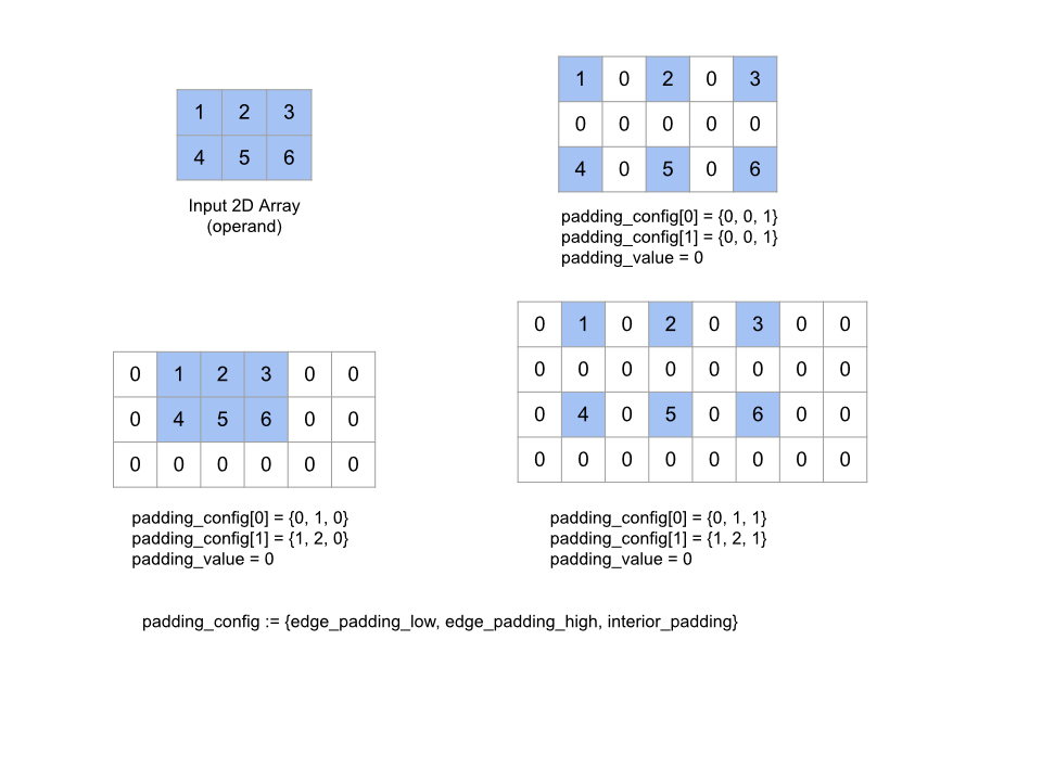
Rozwija podaną tablicę operand przez dopełnienie wokół tablicy, a także między jej elementami za pomocą podanej wartości padding_value. padding_config określa stopień dopełnienia krawędzi i dopełnienia wewnętrznego w przypadku każdego wymiaru.
PaddingConfig to pole powtarzane pola PaddingConfigDimension, które zawiera 3 pola na każdy wymiar: edge_padding_low, edge_padding_high i interior_padding.
edge_padding_low i edge_padding_high określają stopień dopełnienia dodanego odpowiednio na dole (obok indeksu 0) i w najwyższej (obok najwyższego indeksu) każdego wymiaru. Wartość dopełnienia krawędzi może być ujemna – wartość bezwzględna dopełnienia ujemnego wskazuje liczbę elementów do usunięcia z określonego wymiaru.
interior_padding określa stopień dopełnienia dodanego między dowolnymi dwoma elementami w każdym wymiarze. Nie może być ona ujemna. Dopełnienie wewnętrzne odbywa się logicznie przed dopełnieniem krawędzi, dlatego w przypadku takiego dopełnienia elementy są usuwane z operandu z wewnętrzną dopełnieniem.
Ta operacja nie jest operacją, jeśli wszystkie pary dopełnienia krawędzi mają wartość (0, 0), a wartości dopełnienia wewnętrznego mają wartość 0. Poniżej znajdziesz przykłady różnych wartości edge_padding i interior_padding w tablicy dwuwymiarowej.
RecV
Zobacz też XlaBuilder::Recv.
Recv(shape, channel_handle)
| Argumenty | Typ | Semantyka |
|---|---|---|
shape |
Shape |
kształt otrzymywanych danych |
channel_handle |
ChannelHandle |
unikalny identyfikator każdej pary wysyłania/odbierania. |
Odbiera dane o podanym kształcie z instrukcji Send w innych obliczeniach, które mają ten sam uchwyt kanału. Zwraca XlaOp dla odebranych danych.
Interfejs API klienta operacji Recv reprezentuje komunikację synchroniczną.
Instrukcja jest jednak wewnętrznie podzielona na 2 instrukcje HLO (Recv i RecvDone), aby umożliwić asynchroniczne przesyłanie danych. Zobacz też HloInstruction::CreateRecv i HloInstruction::CreateRecvDone.
Recv(const Shape& shape, int64 channel_id)
Przypisuje zasoby wymagane do otrzymywania danych z instrukcji Send z tym samym identyfikatorem channel_id. Zwraca kontekst przydzielonych zasobów, który jest używany przez podaną niżej instrukcję RecvDone, która oczekuje na zakończenie transferu danych. Kontekst jest kropką {receive buffer (shape), request identifier
(U32)} w postaci kropki, która może być używana tylko przez instrukcję RecvDone.
RecvDone(HloInstruction context)
Biorąc pod uwagę kontekst utworzony przez instrukcję Recv, czeka na zakończenie przesyłania danych i zwraca odebrane dane.
Ograniczamy
Zobacz też XlaBuilder::Reduce.
Stosuje funkcję redukcji do co najmniej 1 tablicy równolegle.
Reduce(operands..., init_values..., computation, dimensions)
| Argumenty | Typ | Semantyka |
|---|---|---|
operands |
Kolejność N XlaOp |
N tablic typów T_0, ..., T_{N-1}. |
init_values |
Kolejność N XlaOp |
N skalary typu T_0, ..., T_{N-1}. |
computation |
XlaComputation |
obliczenia typu T_0, ..., T_{N-1}, T_0, ..., T_{N-1} -> Collate(T_0, ..., T_{N-1}). |
dimensions |
Tablica int64 |
nieuporządkowana tablica wymiarów do zredukowania. |
Gdzie:
- Wartość N musi być większa od lub równa 1.
- Obliczenia muszą być w przybliżeniu powiązane (patrz niżej).
- Wszystkie tablice wejściowe muszą mieć te same wymiary.
- Wszystkie wartości początkowe muszą tworzyć tożsamość w elemencie
computation. - Jeśli
N = 1,Collate(T)ma wartośćT. - Jeśli
N > 1,Collate(T_0, ..., T_{N-1})jest kropką elementówNtypuT.
Ta operacja ogranicza co najmniej 1 wymiar każdej tablicy wejściowej do postaci skalarnych.
Pozycja każdej zwróconej tablicy to rank(operand) - len(dimensions). Wynikiem operacji jest Collate(Q_0, ..., Q_N), gdzie Q_i to tablica typu T_i, których wymiary opisano poniżej.
Różne backendy mogą ponownie powiązać obliczenia dotyczące redukcji. Może to prowadzić do różnic liczbowych, ponieważ niektóre funkcje redukcji, takie jak dodawanie, nie są powiązane z liczbami zmiennoprzecinkowymi. Jeśli jednak zakres danych jest ograniczony, dodawanie liczby zmiennoprzecinkowej jest w przypadku większości praktycznych zastosowań zastosowania liczb zmiennoprzecinkowych.
Przykłady
Przy redukcji wartości w jednym wymiarze w pojedynczej tablicy 1D z wartościami [10, 11,
12, 13] przy użyciu funkcji redukcji f (czyli computation), można to obliczyć w ten sposób:
f(10, f(11, f(12, f(init_value, 13)))
ale jest też wiele innych możliwości, np.
f(init_value, f(f(10, f(init_value, 11)), f(f(init_value, 12), f(init_value, 13))))
Poniżej znajduje się skrócony przykład zastosowania redukcji z użyciem sumowania jako obliczenia redukcji z wartością początkową 0.
result_shape <- remove all dims in dimensions from operand_shape

# Iterate over all elements in result_shape. The number of r's here is equal
# to the rank of the result
for r0 in range(result_shape[0]), r1 in range(result_shape[1]), ...:
  # Initialize this result element
  result[r0, r1...] <- 0

  # Iterate over all the reduction dimensions
  for d0 in range(dimensions[0]), d1 in range(dimensions[1]), ...:
    # Increment the result element with the value of the operand's element.
    # The index of the operand's element is constructed from all ri's and di's
    # in the right order (by construction ri's and di's together index over the
    # whole operand shape).
    result[r0, r1...] += operand[ri... di]
Oto przykład redukcji tablicy 2D (macierzy). Kształt ma pozycję 2, wymiar 0 w rozmiarze 2 i wymiar 1 w rozmiarze 3:
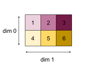
Wyniki zmniejszania wymiarów 0 lub 1 za pomocą funkcji „add”:
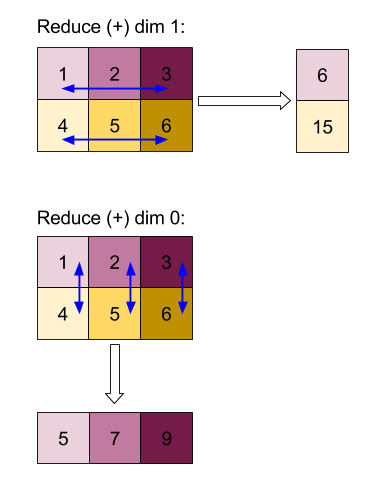
Zwróć uwagę, że oba wyniki redukcji są tablicami 1D. Dla wygody użytkowników na diagramie jedna kolumna jest kolumna, a druga – wierszem.
Bardziej złożony przykład: oto tablica 3D. Jego pozycja to 3, wymiar 0 w rozmiarze 4, wymiar 1 w rozmiarze 2 i wymiar 2 w rozmiarze 3. Dla uproszczenia wartości od 1 do 6 są replikowane w wymiarze 0.
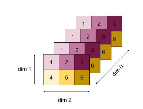
Podobnie jak w przypadku przykładu 2D możemy ograniczyć tylko 1 wymiar. Jeśli na przykład zmniejszymy wymiar 0, uzyskamy tablicę „ranking 2”, w której wszystkie wartości z wymiaru 0 zostaną złożone w postaci skalarnej:
|  4   8  12 |
| 16  20  24 |
Jeśli zmniejszymy wymiar 2, uzyskamy też tablicę rangi 2, w której wszystkie wartości z wymiaru 2 zostaną złożone w skalar:
| 6  15 |
| 6  15 |
| 6  15 |
| 6  15 |
W danych wyjściowych jest zachowywana względna kolejność między pozostałymi wymiarami, ale do niektórych wymiarów mogą zostać przypisane nowe liczby (po zmianie pozycji w rankingu).
Możemy też ograniczyć kilka wymiarów. Dodanie wymiarów 0 i 1 powoduje utworzenie tablicy 1D [20, 28, 36].
Zmniejszenie tablicy 3D do wszystkich jej wymiarów daje skalarny wynik 84.
Redukcja Variadic
W przypadku N > 1 aplikacja funkcji redukcji jest nieco bardziej złożona, ponieważ jest stosowana jednocześnie do wszystkich danych wejściowych. operandy są dostarczane do obliczeń w tej kolejności:
- Działa z zmniejszoną wartością dla pierwszego argumentu
- ...
- Działa zmniejszona wartość dla n-tego argumentu
- Wartość wejściowa pierwszego operandu
- ...
- Wartość wejściowa dla n-tego operandu
Rozważmy na przykład tę funkcję redukcji, za pomocą której można równolegle obliczać wartość maksymalną i argument argmax tablicy 1 D:
f: (Float, Int, Float, Int) -> Float, Int
f(max, argmax, value, index):
  if value >= max:
    return (value, index)
  else:
    return (max, argmax)
W przypadku tablic wejściowych 1D V = Float[N], K = Int[N] i wartości inicjowania I_V = Float, I_K = Int wynik f_(N-1) ograniczania jedynego wymiaru wejściowego jest odpowiednikiem tej aplikacji rekurencyjnej:
f_0 = f(I_V, I_K, V_0, K_0)
f_1 = f(f_0.first, f_0.second, V_1, K_1)
...
f_(N-1) = f(f_(N-2).first, f_(N-2).second, V_(N-1), K_(N-1))
Zastosowanie tego ograniczenia do tablicy wartości i tablicy sekwencyjnych indeksów (tj. iota) spowoduje powtórzenie iteracji w tablicach i zwrócenie kropki zawierającej wartość maksymalną i pasujący indeks.
ReducePrecision
Zobacz też XlaBuilder::ReducePrecision.
Modeluje efekt konwersji wartości zmiennoprzecinkowych na format o niższej dokładności (na przykład IEEE-FP16) i z powrotem do formatu oryginalnego. Liczbę bitów wykładnika i mantysy w formacie o mniejszej dokładności można określić samodzielnie, jednak niektóre rozmiary bitów mogą nie być obsługiwane przez wszystkie implementacje sprzętowe.
ReducePrecision(operand, mantissa_bits, exponent_bits)
| Argumenty | Typ | Semantyka |
|---|---|---|
operand |
XlaOp |
tablica zmiennoprzecinkową typu T. |
exponent_bits |
int32 |
liczba bitów wykładniczych w formacie z mniejszą precyzją |
mantissa_bits |
int32 |
liczba bitów mantissy w formacie o niższej precyzji |
Wynik jest tablicą typu T. Wartości wejściowe są zaokrąglane do najbliższej wartości możliwej do reprezentowania za pomocą podanej liczby bitów mantissy (przy użyciu semantyki „parzystej”), a wszelkie wartości przekraczające zakres określony przez liczbę bitów wykładnika są ograniczane do dodatniej lub ujemnej nieskończoności. NaN wartości są zachowywane, ale mogą zostać przekonwertowane na wartości kanoniczne NaN.
Format o niższej precyzji musi mieć co najmniej 1 bit wykładniczy (aby odróżnić wartość zero od nieskończoności, ponieważ obie mają mantissę zerową) i musi mieć nieujemną liczbę bitów mantissy. Liczba bitów wykładnika lub mantissy może być większa niż wartość odpowiadająca wartości typu T. Odpowiednia część konwersji jest wtedy po prostu niedostępna.
ReduceScatter
Zobacz też XlaBuilder::ReduceScatter.
ReduceScatter to zbiorcza operacja, która skutecznie wykonuje operację AllReduce, a następnie rozkłada wynik, dzieląc go na bloki shard_count wzdłuż scatter_dimension, a replika i w grupie replik otrzymuje fragment ith.
ReduceScatter(operand, computation, scatter_dim, shard_count,
replica_group_ids, channel_id)
| Argumenty | Typ | Semantyka |
|---|---|---|
operand |
XlaOp |
Tablica lub niepusta krotka tablic w celu zmniejszenia liczby replik. |
computation |
XlaComputation |
Obliczanie redukcji |
scatter_dimension |
int64 |
Wymiar do rozproszenia. |
shard_count |
int64 |
Liczba bloków do podziału: scatter_dimension |
replica_groups |
wektor wektorów int64 |
Grupy, w których są stosowane redukcje |
channel_id |
opcjonalnie: int64 |
Opcjonalny identyfikator kanału na potrzeby komunikacji między modułami |
- Gdy
operandjest kropką tablicy, w każdym jej elemencie wykonywana jest metoda redukcji rozproszenia. replica_groupsto lista grup replik, w których przeprowadzana jest redukcja (identyfikator repliki bieżącej repliki można pobrać za pomocąReplicaId). Kolejność replik w każdej grupie określa kolejność, w której zostanie rozproszony wynik całkowitego redukcji.replica_groupsmusi być pusta (w tym przypadku wszystkie repliki należą do jednej grupy) lub zawierać tę samą liczbę elementów co liczba replik. Jeśli istnieje więcej niż 1 grupa replik, wszystkie muszą mieć ten sam rozmiar. Na przykładreplica_groups = {0, 2}, {1, 3}przeprowadza redukcję między replikami0i2, a1i3, a następnie rozprasza wynik.shard_countto rozmiar każdej grupy replik. Jest on potrzebny w sytuacjach, gdy polereplica_groupsjest puste. Jeślireplica_groupsnie jest pusty,shard_countmusi być równy rozmiarowi każdej grupy replik.- Parametr
channel_idsłuży do komunikacji między modułami: tylko operacjereduce-scatterz tym samym atrybutemchannel_idmogą się ze sobą komunikować.
Kształt wyjściowy to taki kształt wejściowy, w którym scatter_dimension pomniejszony jest shard_count razy. Jeśli na przykład są 2 repliki, a operand ma w 2 replikach wartości odpowiednio [1.0, 2.25] i [3.0, 5.25], wartość wyjściowa tej operacji, gdzie scatter_dim to 0, będzie wynosić [4.0] dla pierwszej repliki i [7.5] dla drugiej repliki.
ReduceWindow
Zobacz też XlaBuilder::ReduceWindow.
Stosuje funkcję redukcji do wszystkich elementów w każdym oknie sekwencji N wielowymiarowych tablic, tworząc jako dane wyjściowe 1 lub kropkę N tablic wielowymiarowych. Każda tablica wyjściowa ma taką samą liczbę elementów jak liczba prawidłowych pozycji okna. Warstwa puli może być przedstawiona jako ReduceWindow. Podobnie jak w przypadku Reduce zastosowany computation jest zawsze wyprzedzany przez init_values po lewej stronie.
ReduceWindow(operands..., init_values..., computation, window_dimensions,
window_strides, padding)
| Argumenty | Typ | Semantyka |
|---|---|---|
operands |
N XlaOps |
Sekwencja N wielowymiarowych tablic typów T_0,..., T_{N-1}, z których każda reprezentuje obszar podstawowy, na którym znajduje się okno. |
init_values |
N XlaOps |
Wartości początkowe N zmniejszenia, po jednej dla każdego z N argumentów. Więcej informacji znajdziesz w sekcji Ograniczanie. |
computation |
XlaComputation |
Funkcja redukcji typu T_0, ..., T_{N-1}, T_0, ..., T_{N-1} -> Collate(T_0, ..., T_{N-1}), stosowana do elementów w każdym oknie wszystkich operandów wejściowych. |
window_dimensions |
ArraySlice<int64> |
tablica liczb całkowitych dla wartości wymiarów okna |
window_strides |
ArraySlice<int64> |
tablica liczb całkowitych dla wartości kroku okna |
base_dilations |
ArraySlice<int64> |
tablica liczb całkowitych dla wartości dylatacji bazowej |
window_dilations |
ArraySlice<int64> |
tablica liczb całkowitych dla wartości rozszerzania okna |
padding |
Padding |
typ dopełnienia okna (Dopełnienie::kSame, które dopełnia, aby uzyskać taki sam kształt wyjściowy jak dane wejściowe, jeśli krok ma wartość 1, lub Dopełnienie::kValid, który nie używa dopełnienia i „zatrzymuje” okno, gdy już się nie pasuje) |
Gdzie:
- Wartość N musi być większa od lub równa 1.
- Wszystkie tablice wejściowe muszą mieć te same wymiary.
- Jeśli
N = 1,Collate(T)ma wartośćT. - Jeśli
N > 1,Collate(T_0, ..., T_{N-1})jest kropką elementówNtypu(T0,...T{N-1}).
Poniżej kodu i ilustracji przedstawiono przykład użycia funkcji ReduceWindow. Dane wejściowe to macierz rozmiaru [4 x 6], a atrybuty window_dimension i window_stride_dimension [2 x 3].
// Create a computation for the reduction (maximum).
XlaComputation max;
{
  XlaBuilder builder(client_, "max");
  auto y = builder.Parameter(0, ShapeUtil::MakeShape(F32, {}), "y");
  auto x = builder.Parameter(1, ShapeUtil::MakeShape(F32, {}), "x");
  builder.Max(y, x);
  max = builder.Build().value();
}

// Create a ReduceWindow computation with the max reduction computation.
XlaBuilder builder(client_, "reduce_window_2x3");
auto shape = ShapeUtil::MakeShape(F32, {4, 6});
auto input = builder.Parameter(0, shape, "input");
builder.ReduceWindow(
    input,
    /*init_val=*/builder.ConstantLiteral(LiteralUtil::MinValue(F32)),
    *max,
    /*window_dimensions=*/{2, 3},
    /*window_stride_dimensions=*/{2, 3},
    Padding::kValid);
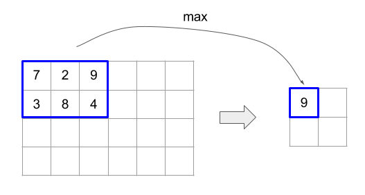
Krok 1 w wymiarze określa, że położenie okna w wymiarze jest o 1 element od sąsiadującego z nim okna. Aby okna nie nakładały się na siebie, parametr window_stride_dimensions powinien być równy wymiarowi window_dimensions. Poniższy rysunek przedstawia wykorzystanie 2 różnych wartości kroku. Dopełnienie jest stosowane do każdego wymiaru danych wejściowych, a obliczenia są takie same, jak gdyby dane wejściowe zostały dostarczone razem z wymiarami po dopełnieniu.
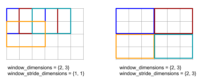
W przypadku prostego dopełnienia spróbuj obliczyć minimalny okres (wartość początkowa to MAX_FLOAT) z wymiarem 3 i przesunąć 2 nad tablicą wejściową [10000, 1000, 100, 10, 1]. Dopełnienie kValid oblicza wartości minimalne w 2 prawidłowych oknach: [10000, 1000, 100] i [100, 10, 1]. Efektem jest wynik [100, 1]. Dopełnienie kSame najpierw wypełnia tablicę, tak aby kształt po oknie redukcji był taki sam jak w przypadku kroku pierwszego. Wystarczy dodać elementy początkowe po obu stronach, uzyskując w ten sposób [MAX_VALUE, 10000, 1000, 100, 10, 1,
MAX_VALUE]. Uruchomienie zmniejszania okna nad tablicą z dopełnieniem działa w 3 oknach [MAX_VALUE, 10000, 1000], [1000, 100, 10], [10, 1, MAX_VALUE] i [1000, 10, 1].
Kolejność oceny funkcji redukcji jest dowolna i może nie być deterministyczna. Dlatego funkcja redukcji nie powinna być zbyt czuła na ponowne powiązanie. Więcej informacji znajdziesz w sekcji o powiązaniach w kontekście modelu Reduce.
ReplicaId
Zobacz też XlaBuilder::ReplicaId.
Zwraca unikalny identyfikator (skalarny U32) repliki.
ReplicaId()
Unikalny identyfikator każdej repliki jest nieoznaczoną liczbą całkowitą z przedziału [0, N), gdzie N to liczba replik. Ponieważ wszystkie repliki korzystają z tego samego programu, wywołanie ReplicaId() w programie zwróci inną wartość dla każdej repliki.
Zmień kształt
Zobacz też XlaBuilder::Reshape i operację Collapse.
Zmienia wymiary tablicy w nową konfigurację.
Reshape(operand, new_sizes)
Reshape(operand, dimensions, new_sizes)
| Argumenty | Typ | Semantyka |
|---|---|---|
operand |
XlaOp |
tablica typu T |
dimensions |
Wektor int64 |
kolejność zwiniętych wymiarów. |
new_sizes |
Wektor int64 |
wektor rozmiarów nowych wymiarów |
W kontekście zmiana kształtu najpierw spłaszcza tablicę do jednowymiarowego wektora z wartościami danych, a następnie doprecyzowuje ten wektor do nowego kształtu. Argumenty wejściowe to dowolna tablica typu T, wektor o stałym czasie kompilowania indeksów wymiarów i wektor stałego w czasie kompilacji danych o rozmiarach.
Wartości we wektorze dimension, jeśli podano, muszą być permutacją wszystkich wymiarów T. Jeśli nie podano wartości domyślnej, jest to {0, ..., rank - 1}. Kolejność wymiarów w funkcji dimensions jest uzależniona od wymiaru najniższego (największego) do najmniejszego wymiaru (największy z największym drobnym) w gnieździe pętli, który zwija tablicę wejściową do jednego wymiaru. Wektor new_sizes określa rozmiar tablicy wyjściowej. Wartość w indeksie 0 w argumencie new_sizes to rozmiar wymiaru 0, wartość w indeksie 1 to rozmiar wymiaru 1 itd. Iloczyn wymiarów new_size musi być równy iloczynowi rozmiarów wymiarów operandu. Podczas precyzowania zwiniętej tablicy do tablicy wielowymiarowej zdefiniowanej przez funkcję new_sizes wymiary w new_sizes są uporządkowane od najmniejszej (największej) do najmniejszej zmiennej (największe drobne).
Na przykład niech v będzie tablicą 24 elementów:
let v = f32[4x2x3] { { {10, 11, 12}, {15, 16, 17} },
                    { {20, 21, 22}, {25, 26, 27} },
                    { {30, 31, 32}, {35, 36, 37} },
                    { {40, 41, 42}, {45, 46, 47} } };

In-order collapse:
let v012_24 = Reshape(v, {0,1,2}, {24});
then v012_24 == f32[24] {10, 11, 12, 15, 16, 17, 20, 21, 22, 25, 26, 27,
                         30, 31, 32, 35, 36, 37, 40, 41, 42, 45, 46, 47};

let v012_83 = Reshape(v, {0,1,2}, {8,3});
then v012_83 == f32[8x3] { {10, 11, 12}, {15, 16, 17},
                          {20, 21, 22}, {25, 26, 27},
                          {30, 31, 32}, {35, 36, 37},
                          {40, 41, 42}, {45, 46, 47} };

Out-of-order collapse:
let v021_24 = Reshape(v, {1,2,0}, {24});
then v012_24 == f32[24]  {10, 20, 30, 40, 11, 21, 31, 41, 12, 22, 32, 42,
                          15, 25, 35, 45, 16, 26, 36, 46, 17, 27, 37, 47};

let v021_83 = Reshape(v, {1,2,0}, {8,3});
then v021_83 == f32[8x3] { {10, 20, 30}, {40, 11, 21},
                          {31, 41, 12}, {22, 32, 42},
                          {15, 25, 35}, {45, 16, 26},
                          {36, 46, 17}, {27, 37, 47} };


let v021_262 = Reshape(v, {1,2,0}, {2,6,2});
then v021_262 == f32[2x6x2] { { {10, 20}, {30, 40},
                              {11, 21}, {31, 41},
                              {12, 22}, {32, 42} },
                             { {15, 25}, {35, 45},
                              {16, 26}, {36, 46},
                              {17, 27}, {37, 47} } };
W szczególnym przypadku funkcja rekształtowania może przekształcić tablicę z jednym elementem w skalar i na odwrót. Przykład:
Reshape(f32[1x1] { {5} }, {0,1}, {}) == 5;
Reshape(5, {}, {1,1}) == f32[1x1] { {5} };
Obr. (odwrócone)
Zobacz też XlaBuilder::Rev.
Rev(operand, dimensions)
| Argumenty | Typ | Semantyka |
|---|---|---|
operand |
XlaOp |
tablica typu T |
dimensions |
ArraySlice<int64> |
wymiary do odwrócenia |
Odwraca kolejność elementów w tablicy operand wzdłuż podanej wartości dimensions, generując tablicę wyjściową o tym samym kształcie. Każdy element tablicy operandu w indeksie wielowymiarowym jest przechowywany w tablicy wyjściowej w przekształconym indeksie. Indeks wielowymiarowy jest przekształcany przez odwrócenie indeksu w każdym wymiarze, który ma być odwrócony (np. jeśli wymiar rozmiaru N jest jednym z wymiarów odwróconych, jego indeks i zostanie przekształcony w N–1–i).
Operacja Rev polega na odwróceniu tablicy wagi splotu wzdłuż 2 wymiarów okna podczas obliczania gradientu w sieciach neuronowych.
RngNormal
Zobacz też XlaBuilder::RngNormal.
Konstruuje dane wyjściowe o danym kształcie z liczbami losowymi wygenerowanymi zgodnie z rozkładem normalnym \(N(\mu, \sigma)\) . Parametry \(\mu\) , \(\sigma\)i kształt wyjściowy muszą mieć typ elementu zmiennoprzecinkowego. Dodatkowo parametry muszą mieć wartość skalarną.
RngNormal(mu, sigma, shape)
| Argumenty | Typ | Semantyka |
|---|---|---|
mu |
XlaOp |
Skalar typu T określająca średnią wygenerowanych liczb |
sigma |
XlaOp |
Skalowalna typu T określająca odchylenie standardowe wygenerowanego |
shape |
Shape |
Kształt wyjściowy typu T |
RngUniform
Zobacz też XlaBuilder::RngUniform.
Konstruuje dane wyjściowe o danym kształcie z losowymi liczbami wygenerowanymi po równomiernym rozkładzie w przedziale \([a,b)\). Parametry i typ elementu wyjściowego muszą być wartością logiczną, całkowitą lub zmiennoprzecinkową, a typy muszą być spójne. Backendy procesora i GPU obsługują obecnie tylko modele F64, F32, F16, BF16, S64, U64, S32 i U32. Ponadto parametry muszą mieć wartość skalarną. Jeśli \(b <= a\) wynik jest zdefiniowany przez implementację.
RngUniform(a, b, shape)
| Argumenty | Typ | Semantyka |
|---|---|---|
a |
XlaOp |
Skalar typu T określający dolny limit interwału |
b |
XlaOp |
Skalowalna typu T określająca górny limit interwału |
shape |
Shape |
Kształt wyjściowy typu T |
RngBitGenerator
Generuje dane wyjściowe o danym kształcie wypełnionym jednolitymi losowymi bitami za pomocą określonego algorytmu (lub domyślnego backendu) i zwraca zaktualizowany stan (o tym samym kształcie co stan początkowy) oraz wygenerowane dane losowe.
Stan początkowy to stan początkowy bieżącego generowania liczb losowych. Jego wymagany kształt i prawidłowe wartości zależą od zastosowanego algorytmu.
Gwarantujemy, że dane wyjściowe będą deterministyczną funkcją stanu początkowego, ale nie można mieć pewności, że będą deterministyczne między backendami a różnymi wersjami kompilatora.
RngBitGenerator(algorithm, key, shape)
| Argumenty | Typ | Semantyka |
|---|---|---|
algorithm |
RandomAlgorithm |
Algorytm PRNG, który ma zostać użyty. |
initial_state |
XlaOp |
Stan początkowy algorytmu PRNG. |
shape |
Shape |
Kształt danych wyjściowych generowanych danych. |
Dostępne wartości parametru algorithm:
rng_default: algorytm dla backendu z wymaganiami dotyczącymi kształtów określonych dla backendu.rng_three_fry: algorytm PRNG oparty na liczniku ThreeFry. Kształtinitial_statetou64[2]z dowolnymi wartościami. Salmon i in. SC 2011. Równoległe liczby losowe: tak proste jak 1, 2, 3.rng_philox: algorytm Philox do równoległego generowania liczb losowych. Kształtinitial_statema postaću64[3]z dowolnymi wartościami. Salmon i in. SC 2011. Równoległe liczby losowe: tak proste jak 1, 2, 3.
Punktowy
Operacja rozproszenia XLA generuje sekwencję wyników, które są wartościami tablicy wejściowej operands, z kilkoma wycinkami (w indeksach określonych przez scatter_indices) aktualizowanymi sekwencją wartości w updates za pomocą metody update_computation.
Zobacz też XlaBuilder::Scatter.
scatter(operands..., scatter_indices, updates..., update_computation,
index_vector_dim, update_window_dims, inserted_window_dims,
scatter_dims_to_operand_dims)
| Argumenty | Typ | Semantyka |
|---|---|---|
operands |
Kolejność N XlaOp |
N tablic typów T_0, ..., T_N, w których ma zostać rozproszony element. |
scatter_indices |
XlaOp |
Tablica zawierająca początkowe indeksy wycinków, które muszą zostać rozproszone. |
updates |
Kolejność N XlaOp |
N tablic typów T_0, ..., T_N. updates[i] zawiera wartości, które należy wykorzystać do rozproszenia elementu operands[i]. |
update_computation |
XlaComputation |
Obliczenie, które ma służyć do łączenia istniejących wartości w tablicy wejściowej i aktualizacji w trakcie rozproszenia. Obliczenia powinny być typu T_0, ..., T_N, T_0, ..., T_N -> Collate(T_0, ..., T_N). |
index_vector_dim |
int64 |
Wymiar w tabeli scatter_indices zawierający początkowe indeksy. |
update_window_dims |
ArraySlice<int64> |
Zestaw wymiarów w kształcie updates, które są wymiarami okien. |
inserted_window_dims |
ArraySlice<int64> |
Zestaw wymiarów okien, które należy wstawić dla kształtu updates. |
scatter_dims_to_operand_dims |
ArraySlice<int64> |
Wymiary są mapowane od indeksów punktowych do przestrzeni indeksu argumentów. Ta tablica jest interpretowana jako mapowanie i na scatter_dims_to_operand_dims[i] . Musi mieć wartość jeden do jednego w całości. |
indices_are_sorted |
bool |
Określa, czy indeksy zostaną posortowane według elementu wywołującego. |
Gdzie:
- Wartość N musi być większa od lub równa 1.
operands[0], ...,operands[N-1] muszą mieć te same wymiary.updates[0], ...,updates[N-1] muszą mieć te same wymiary.- Jeśli
N = 1,Collate(T)ma wartośćT. - Jeśli
N > 1,Collate(T_0, ..., T_N)jest kropką elementówNtypuT.
Jeśli index_vector_dim ma wartość scatter_indices.rank, domyślnie uznajemy, że parametr scatter_indices ma na końcu wymiar 1.
Definiujemy update_scatter_dims typu ArraySlice<int64> jako zbiór wymiarów o kształcie updates, które nie są podane w formacie update_window_dims, w kolejności rosnącej.
Argumenty funkcji rozproszenia powinny być zgodne z tymi ograniczeniami:
Każda tablica
updatesmusi mieć pozycjęupdate_window_dims.size + scatter_indices.rank - 1.Ograniczenia wymiaru
iw każdej tablicyupdatesmuszą być zgodne z tymi zasadami:- Jeśli właściwość
iwystępuje w elemencieupdate_window_dims(czyli równa sięupdate_window_dims[k] w przypadku niektórychk), to granica wymiaruiwupdatesnie może przekraczać odpowiadającej mu granicy wymiaruipo uwzględnieniu parametruinserted_window_dims(czyliadjusted_window_bounds[k], gdzieadjusted_window_boundszawiera graniceoperandz usuniętymi granicami w indeksachinserted_window_dims).operand - Jeśli element
iwystępuje w elemencieupdate_scatter_dims(czyli równa sięupdate_scatter_dims[k] w przypadku niektórych rodzajów danychk), to granica wymiaruiw parametrzeupdatesmusi być równa odpowiadającej mu granicy z parametremscatter_indices, z pominięciem wartościindex_vector_dim(tzn.scatter_indices.shape.dims[k], jeślik<index_vector_dim, ascatter_indices.shape.dims[k+1] – inaczej).
- Jeśli właściwość
update_window_dimsmusi mieć kolejność rosnącą, nie może zawierać powtarzających się numerów wymiarów i znajdować się w zakresie[0, updates.rank).inserted_window_dimsmusi mieć kolejność rosnącą, nie może zawierać powtarzających się numerów wymiarów i znajdować się w zakresie[0, operand.rank).operand.rankmusi być równy sumie wartościupdate_window_dims.sizeiinserted_window_dims.size.scatter_dims_to_operand_dims.sizemusi być równyscatter_indices.shape.dims[index_vector_dim], a jego wartości muszą mieścić się w zakresie[0, operand.rank).
W przypadku danego indeksu U w każdej tablicy updates odpowiedni indeks I w odpowiedniej tablicy operands, do której należy zastosować tę aktualizację, jest obliczany w ten sposób:
- Niech
G= {U[k] dlakwupdate_scatter_dims}. Użyj funkcjiG, aby wyszukać wektor indeksuSw tablicyscatter_indicestak, abyS[i] =scatter_indices[Połącz(G,i)], gdzie Łączenie(A, b) wstawia b w pozycjiindex_vector_dimdo A. - Utwórz indeks
Sinw miejscu:operandprzy użyciu polaS, rozpraszając obszarSna mapiescatter_dims_to_operand_dims. Bardziej formalnie:Sin[scatter_dims_to_operand_dims[k]] =S[k], jeślik<scatter_dims_to_operand_dims.size.Sin[_] =0w innym przypadku.
- Utwórz indeks
Winw każdej tablicyoperands, rozpraszając indeksy w miejscuupdate_window_dimsw tabeliUzgodnie zinserted_window_dims. Bardziej formalnie:Win[window_dims_to_operand_dims(k)] =U[k], jeślikjest w elemencieupdate_window_dims, gdziewindow_dims_to_operand_dimsto funkcja monotoniczna z domeną [0,update_window_dims.size) i zakresem [0,operand.rank) \inserted_window_dims. Jeśli np.update_window_dims.sizeto4,operand.rankto6, ainserted_window_dimsto {0,2}, towindow_dims_to_operand_dimsto {0→1,1→3,2→4,3→5}.Win[_] =0w innym przypadku.
ItoWin+Sin, gdzie + oznacza dodawanie na podstawie elementu.
Podsumowując, operację rozproszenia można zdefiniować w ten sposób.
- Zainicjuj
outputprzy użyciu funkcjioperands, czyli dla wszystkich indeksówJdla wszystkich indeksówOw tablicyoperands[J]:
output[J][O] =operands[J][O] - Dla każdego indeksu
Uw tablicyupdates[J] i odpowiadającego mu indeksuOw tablicyoperand[J], jeśliOjest prawidłowym indeksem dlaoutput:
(output[0][O], ...,output[N-1][O]) =update_computation(output[0][O], ..., ,output[N-1][O],updates[0][U], ...,updates[N-1][U])
Kolejność stosowania aktualizacji nie jest deterministyczna. Jeśli więc wiele indeksów w updates odnosi się do tego samego indeksu w metodzie operands, odpowiadająca jej wartość w funkcji output będzie niedeterministyczna.
Pamiętaj, że pierwszy parametr przekazywany do funkcji update_computation jest zawsze wartością bieżącą z tablicy output, a drugi – wartością z tablicy updates. Jest to ważne zwłaszcza w przypadkach, gdy właściwość update_computation nie jest przemienna.
Jeśli zasada indices_are_sorted ma wartość Prawda, XLA może założyć, że elementy start_indices są posortowane (w kolejności start_index_map) według użytkownika. W przeciwnym razie
określona jest semantyka.
Operacja rozproszenia może być postrzegana jako odwrotność operacji zbierania, tj. operacja rozproszenia aktualizuje elementy w danych wejściowych, które zostały wyodrębnione przez odpowiednią operację zbierania.
Szczegółowy nieformalny opis i przykłady znajdziesz w sekcji „Informacyjny opis” na stronie Gather.
Wybierz
Zobacz też XlaBuilder::Select.
Konstruuje tablicę wyjściową z elementów 2 tablic wejściowych na podstawie wartości tablicy predykatu.
Select(pred, on_true, on_false)
| Argumenty | Typ | Semantyka |
|---|---|---|
pred |
XlaOp |
tablica typu PRED |
on_true |
XlaOp |
tablica typu T |
on_false |
XlaOp |
tablica typu T |
Tablice on_true i on_false muszą mieć ten sam kształt. Taki jest też kształt tablicy wyjściowej. Tablica pred musi mieć tę samą wymiary co on_true i on_false, a jej typ elementu to PRED.
Dla każdego elementu P elementu pred odpowiedni element tablicy wyjściowej jest pobierany z on_true, jeśli wartość P wynosi true, lub z on_false, jeśli wartość P to false. Jako ograniczonej formy transmisji pred może być skalarem typu PRED. W tym przypadku tablica wyjściowa jest pobierana w całości z elementu on_true, jeśli pred ma wartość true, lub z on_false, jeśli pred to false.
Przykład z wartością pred nieskalarną:
let pred: PRED[4] = {true, false, false, true};
let v1: s32[4] = {1, 2, 3, 4};
let v2: s32[4] = {100, 200, 300, 400};
==>
Select(pred, v1, v2) = s32[4]{1, 200, 300, 4};
Przykład ze skalarnym pred:
let pred: PRED = true;
let v1: s32[4] = {1, 2, 3, 4};
let v2: s32[4] = {100, 200, 300, 400};
==>
Select(pred, v1, v2) = s32[4]{1, 2, 3, 4};
Obsługiwany jest wybór między krotkami. W tym celu krotki są uznawane za typy skalarne. Jeśli on_true i on_false są krotkami (które muszą mieć taki sam kształt), to pred musi być skalarem typu PRED.
SelectAndScatter
Zobacz też XlaBuilder::SelectAndScatter.
Tę operację można uznać za operację złożoną, gdy najpierw oblicza wartość ReduceWindow w tablicy operand, aby wybrać element z każdego okna, a potem rozkłada tablicę source na indeksy wybranych elementów, aby utworzyć tablicę wyjściową o tym samym kształcie co tablica argumentów. Funkcja select umożliwia wybranie elementu z każdego okna przez zastosowanie go w każdym z nich. Jest ona wywoływana za pomocą właściwości, według której wektor indeksu pierwszego parametru jest leksykograficznie mniejszy niż wektor indeksu drugiego parametru. Funkcja select zwraca wartość true, jeśli wybrany jest pierwszy parametr, i zwraca false, jeśli wybrano drugi, a funkcja musi utrzymywać przechodność (np. jeśli select(a, b) i select(b, c) mają wartość true, a select(a, c) to również true), tak aby wybrany element nie zależy od kolejności elementów przemierzonych w danym oknie.
Funkcja scatter jest stosowana przy każdym wybranym indeksie w tablicy wyjściowej. Uwzględnia 2 parametry skalarne:
- Bieżąca wartość w wybranym indeksie w tablicy wyjściowej
- Wartość punktowa z kolumny
sourcedotycząca wybranego indeksu
Łączy on 2 parametry i zwraca wartość skalarną używaną do aktualizacji wartości w wybranym indeksie w tablicy wyjściowej. Początkowo wszystkie indeksy tablicy wyjściowej mają wartość init_value.
Tablica wyjściowa ma ten sam kształt co tablica operand, a tablica source musi mieć ten sam kształt w wyniku zastosowania operacji ReduceWindow na tablicy operand. SelectAndScatter może posłużyć do cofania się wartości gradientu w warstwie puli w sieci neuronowej.
SelectAndScatter(operand, select, window_dimensions, window_strides,
padding, source, init_value, scatter)
| Argumenty | Typ | Semantyka |
|---|---|---|
operand |
XlaOp |
tablica typu T, po której przesuwane są okna |
select |
XlaComputation |
obliczenia binarne typu T, T -> PRED, które mają zastosowanie do wszystkich elementów w każdym oknie; zwraca wartość true, jeśli wybrano pierwszy parametr, i zwraca false, jeśli wybrano drugi parametr |
window_dimensions |
ArraySlice<int64> |
tablica liczb całkowitych dla wartości wymiarów okna |
window_strides |
ArraySlice<int64> |
tablica liczb całkowitych dla wartości kroku okna |
padding |
Padding |
typ dopełnienia okna (Dopełnienie::kSame lub Dopełnienie::kValid) |
source |
XlaOp |
tablica typu T z wartościami do rozproszenia |
init_value |
XlaOp |
wartość skalarna typu T dla wartości początkowej tablicy wyjściowej |
scatter |
XlaComputation |
obliczenia binarne typu T, T -> T w celu zastosowania każdego elementu źródłowego z rozproszeniami z jego elementem docelowym |
Poniższy rysunek przedstawia przykłady użycia funkcji SelectAndScatter, gdzie funkcja select oblicza maksymalną wartość spośród jej parametrów. Pamiętaj, że gdy okna się nakładają, tak jak na ilustracji (2) poniżej, indeks tablicy operand może zostać wybrany kilka razy przez różne okna. Na ilustracji element wartości 9 jest wybierany przez górne okna (niebieski i czerwony), a funkcja dodawania binarnego scatter tworzy element wyjściowy o wartości 8 (2 + 6).
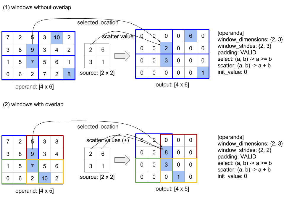
Kolejność oceny funkcji scatter jest dowolna i może nie być deterministyczna. Z tego powodu funkcja scatter nie powinna być zbyt czuła na ponowne powiązanie. Więcej informacji znajdziesz w sekcji o powiązaniach w kontekście modelu Reduce.
Wyślij
Zobacz też XlaBuilder::Send.
Send(operand, channel_handle)
| Argumenty | Typ | Semantyka |
|---|---|---|
operand |
XlaOp |
dane do wysłania (tablica typu T) |
channel_handle |
ChannelHandle |
unikalny identyfikator każdej pary wysyłania/odbierania. |
Wysyła podane dane argumentu do instrukcji Recv w innych obliczeniach, które mają ten sam uchwyt kanału. Nie zwraca żadnych danych.
Podobnie jak w przypadku Recv, interfejs API klienta operacji Send reprezentuje komunikację synchronizację i jest wewnętrznie podzielony na 2 instrukcje HLO (Send i SendDone), aby umożliwić asynchroniczne przesyłanie danych. Zobacz też HloInstruction::CreateSend i HloInstruction::CreateSendDone.
Send(HloInstruction operand, int64 channel_id)
Inicjuje asynchroniczne przesyłanie operandu do zasobów przydzielonych przez instrukcję Recv z tym samym identyfikatorem kanału. Zwraca kontekst, który jest używany przez podaną niżej instrukcję SendDone, która czeka na zakończenie przenoszenia danych. Kontekst jest kropką {operand (shape), identyfikator żądania (U32)}, którego można używać tylko przez instrukcję SendDone.
SendDone(HloInstruction context)
Biorąc pod uwagę kontekst utworzony przez instrukcję Send, oczekuje na zakończenie przesyłania danych. Instrukcja nie zwraca żadnych danych.
Ustalanie harmonogramu instrukcji dla kanału
Kolejność wykonania 4 instrukcji dla każdego kanału (Recv, RecvDone,
Send, SendDone) jest taka sama jak poniżej.
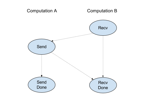
Recvma miejsce przedSendSendma miejsce przedRecvDoneRecvma miejsce przedRecvDoneSendma miejsce przedSendDone
Gdy kompilatory backendu generują liniowy harmonogram dla wszystkich obliczeń, które komunikują się zgodnie z instrukcjami dotyczącymi kanału, nie mogą występować cykle między obliczeniami. Na przykład poniższe harmonogramy prowadzą do zakleszczenia.
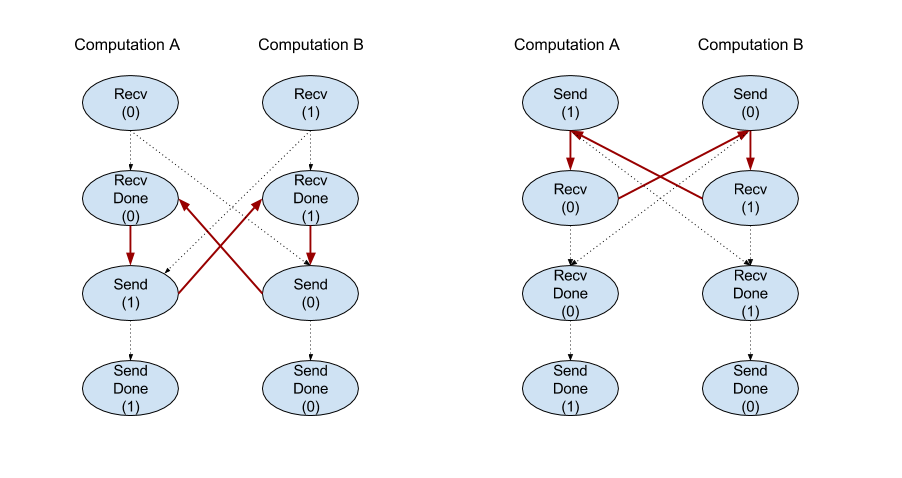
Wycinek
Zobacz też XlaBuilder::Slice.
Wyodrębnianie macierzy podrzędnej z tablicy wejściowej. Tablica podrzędna ma taką samą pozycję jak dane wejściowe i zawiera wartości wewnątrz ramki ograniczającej w tablicy wejściowej, gdzie wymiary i indeksy ramki ograniczającej są podane jako argumenty operacji wycinka.
Slice(operand, start_indices, limit_indices, strides)
| Argumenty | Typ | Semantyka |
|---|---|---|
operand |
XlaOp |
N tablica wymiarowa typu T |
start_indices |
ArraySlice<int64> |
Lista N liczb całkowitych zawierających początkowe indeksy wycinka dla każdego wymiaru. Wartości nie mogą być większe niż 0. |
limit_indices |
ArraySlice<int64> |
Lista N liczb całkowitych zawierających końcowe indeksy (wyłącznie) na wycinku każdego wymiaru. Każda wartość musi być większa lub równa odpowiedniej wartości start_indices dla wymiaru oraz mniejsza lub równa rozmiarowi wymiaru. |
strides |
ArraySlice<int64> |
Lista N liczb całkowitych, które decydują o kroku wejściowego wycinka. Wycinek wybiera każdy element strides[d] w wymiarze d. |
Przykład jednowymiarowy:
let a = {0.0, 1.0, 2.0, 3.0, 4.0}
Slice(a, {2}, {4}) produces:
  {2.0, 3.0}
Przykład obrazu dwuwymiarowego:
let b =
 { {0.0,  1.0,  2.0},
   {3.0,  4.0,  5.0},
   {6.0,  7.0,  8.0},
   {9.0, 10.0, 11.0} }

Slice(b, {2, 1}, {4, 3}) produces:
  { { 7.0,  8.0},
    {10.0, 11.0} }
Sortuj
Zobacz też XlaBuilder::Sort.
Sort(operands, comparator, dimension, is_stable)
| Argumenty | Typ | Semantyka |
|---|---|---|
operands |
ArraySlice<XlaOp> |
operandy do sortowania. |
comparator |
XlaComputation |
Wartość porównawcza do użycia. |
dimension |
int64 |
Wymiar, według którego następuje sortowanie. |
is_stable |
bool |
Określa, czy należy używać sortowania stabilnego. |
Jeśli podasz tylko 1 operand:
Jeśli operand jest tensorem rankingu 1 (tablica), wynik jest posortowaną tablicą. Jeśli chcesz posortować tablicę w kolejności rosnącej, funkcja porównywania powinna wykonać porównanie z wartością mniejszą niż. Formalnie po posortowaniu tablicy tablica ta utrzymuje się na wszystkich pozycjach indeksu
i, jz wartościąi < jo wartościcomparator(value[i], value[j]) = comparator(value[j], value[i]) = falselubcomparator(value[i], value[j]) = true.Jeśli operand ma wyższą pozycję w rankingu, jest on sortowany według podanego wymiaru. Na przykład w przypadku tensora rankingu 2 (macierzy) wartość wymiaru
0będzie niezależnie sortować każdą kolumnę, a wartość wymiaru1będzie niezależnie sortować każdy wiersz. Jeśli nie podasz numeru wymiaru, domyślnie zostanie wybrany ostatni wymiar. W przypadku posortowanego wymiaru obowiązuje taka sama kolejność sortowania jak w przypadku argumentu „ranking 1”.
Jeśli podane są operandy n > 1:
Wszystkie operandy
nmuszą być tensorami o tych samych wymiarach. Typy elementów tensorów mogą być różne.Wszystkie operandy są sortowane razem, a nie pojedynczo. operandy są z założenia traktowane jako krotki. Podczas sprawdzania, czy elementy każdego operandu na pozycjach
iijmuszą zostać zamienione, komparator jest wywoływany z parametrami skalarnymi2 * n, gdzie parametr2 * kodpowiada wartości na pozycjiiz operanduk-th, a parametr2 * k + 1odpowiada wartości w pozycjijz operanduk-th. Zwykle funkcja porównywania pozwala ze sobą porównać parametry2 * ki2 * k + 1, a potem wykorzystać inne pary parametrów jako elementy decydujące.Wynikiem jest krotka, która składa się z operandów w posortowanej kolejności (wzdłuż podanego wymiaru, jak powyżej). Argument
i-thkrotki odpowiada operandowii-thtypu Sort.
Jeśli są np. 3 operandy operand0 = [3, 1], operand1 = [42, 50] i operand2 = [-3.0, 1.1], a komparator porównuje tylko wartości operand0 z mniejszą wartością, wynik sortowania to kropka ([1, 3], [50, 42], [1.1, -3.0]).
Jeśli zasada is_stable ma wartość Prawda, gwarantowane sortowanie jest stabilne, czyli jeśli istnieją elementy, które komparator uzna, że są równe, obowiązuje względna kolejność równych wartości. 2 elementy e1 i e2 są równe
tylko wtedy, gdy comparator(e1, e2) = comparator(e2, e1) = false. Domyślnie is_stable ma wartość Fałsz.
Transponuj
Zobacz też operację tf.reshape.
Transpose(operand)
| Argumenty | Typ | Semantyka |
|---|---|---|
operand |
XlaOp |
Argument do transponowania. |
permutation |
ArraySlice<int64> |
Jak permutować wymiary. |
Permutuje wymiary operandu za pomocą danej permutacji, więc ∀ i . 0 ≤ i < rank ⇒ input_dimensions[permutation[i]] = output_dimensions[i].
Ta funkcja działa tak samo jak Reshape(operand, permutation, Permute(permutation, operand.shape.dimensions)).
TriangularSolve
Zobacz też XlaBuilder::TriangularSolve.
Rozwiązanie układów równań liniowych o dolnym lub górnym współczynniku trójkątnym przez podstawienie do przodu lub wstecz. Ta rutyna, która przesyła dane zgodnie z wymiarami wiodącymi, rozwiązuje jeden z układów macierzy op(a) * x =
b lub x * op(a) = b dla zmiennej x z danymi a i b, gdzie op(a) to op(a) = a, op(a) = Transpose(a) lub op(a) = Conj(Transpose(a)).
TriangularSolve(a, b, left_side, lower, unit_diagonal, transpose_a)
| Argumenty | Typ | Semantyka |
|---|---|---|
a |
XlaOp |
tablica > 2 typu zespolonego lub zmiennoprzecinkowego o kształcie [..., M, M]. |
b |
XlaOp |
tablica o rankingu > 2 tego samego typu z kształtem [..., M, K], jeśli zasada left_side ma wartość prawda. W przeciwnym razie [..., K, M]. |
left_side |
bool |
wskazuje, czy należy rozwiązać układ o postaci op(a) * x = b (true) czy x * op(a) = b (false). |
lower |
bool |
określa, czy użyć górnego, czy dolnego trójkąta a. |
unit_diagonal |
bool |
jeśli ustawiona jest wartość true, przyjmuje się, że elementy a po przekątnej mają wartość 1 i nie są otwierane. |
transpose_a |
Transpose |
czy użyć elementu a w obecnej postaci, przetransponować go lub użyć jego sprzężonego transponowania. |
Dane wejściowe są odczytywane tylko z górnego/dolnego trójkąta a (w zależności od wartości lower). Wartości z drugiego trójkąta są ignorowane. Dane wyjściowe są zwracane w tym samym trójkącie. Wartości w drugim trójkącie są zdefiniowane przez implementację i mogą być dowolne.
Jeśli pozycje a i b mają wartość większą niż 2, są one traktowane jak wsady macierzy, gdzie wszystkie oprócz 2 podrzędnych wymiarów są wymiarami wsadowymi. a i b muszą mieć jednakowe wymiary wsadu.
Kropka
Zobacz też XlaBuilder::Tuple.
Kropka zawierająca zmienną liczbę nicków danych, z których każdy ma własny kształt.
Jest to odpowiednik std::tuple w C++. Koncepcyjnie:
let v: f32[10] = f32[10]{0, 1, 2, 3, 4, 5, 6, 7, 8, 9};
let s: s32 = 5;
let t: (f32[10], s32) = tuple(v, s);
Kropki można zdekonstruować (dotrzeć do nich) za pomocą operacji GetTupleElement.
Gdy
Zobacz też XlaBuilder::While.
While(condition, body, init)
| Argumenty | Typ | Semantyka |
|---|---|---|
condition |
XlaComputation |
XlaComputation typu T -> PRED, który określa warunek zakończenia pętli. |
body |
XlaComputation |
XlaComputation typu T -> T, który określa treść pętli. |
init |
T |
Początkowa wartość parametru condition i body. |
Wykonuje kolejno body, aż do wystąpienia błędu condition. Przypomina to typową pętlę pętli w wielu innych językach. Wyjątkiem są różnice i ograniczenia wymienione poniżej.
- Węzeł
Whilezwraca wartość typuT, która jest wynikiem ostatniego wykonania poleceniabody. - Kształt typu
Tjest określony statycznie i musi być taki sam we wszystkich iteracjach.
Parametry T obliczeń są inicjowane z wartością init w pierwszej iteracji i przy każdej kolejnej iteracji automatycznie aktualizowane są do nowego wyniku z body.
Jednym z głównych przypadków użycia węzła While jest implementacja powtórzonego trenowania w sieciach neuronowych. Poniżej znajduje się uproszczony pseudokod wraz z wykresem przedstawiającym obliczenia. Kod znajdziesz tutaj: while_test.cc.
W tym przykładzie typ T to Tuple, składający się z int32 oznacza liczbę iteracji i vector[10] (zasobnik). W przypadku 1000 iteracji pętla dodaje do akumulatora stały wektor.
// Pseudocode for the computation.
init = {0, zero_vector[10]} // Tuple of int32 and float[10].
result = init;
while (result(0) < 1000) {
  iteration = result(0) + 1;
  new_vector = result(1) + constant_vector[10];
  result = {iteration, new_vector};
}
