Di seguito viene descritta la semantica delle operazioni definita nell'interfaccia XlaBuilder. In genere, queste operazioni mappano one-to-one alle operazioni definite
nell'interfaccia RPC in
xla_data.proto.
Una nota sulla nomenclatura: il tipo di dati generalizzati con cui si occupa XLA è un array N-dimensionale che contiene elementi di tipo uniforme (come il valore in virgola mobile a 32 bit). In tutta la documentazione, viene utilizzato array per indicare un array dimensionale arbitrario. Per praticità, i casi speciali hanno nomi più specifici e familiari; ad esempio, un vettore è una matrice unidimensionale e una matrice è una matrice bidimensionale.
AfterAll
Vedi anche
XlaBuilder::AfterAll.
AfterAll utilizza un numero variadic di token e produce un singolo token. I token sono tipi primitivi che possono essere raggruppati tra operazioni con effetti collaterali per applicare l'ordine. AfterAll può essere utilizzato come join di token per ordinare un'operazione dopo un'operazione impostata.
AfterAll(operands)
| Argomenti | Tipo | Semantica |
|---|---|---|
operands |
XlaOp |
numero variadic di token |
AllGather
Vedi anche
XlaBuilder::AllGather.
Esegue la concatenazione tra le repliche.
AllGather(operand, all_gather_dim, shard_count, replica_group_ids,
channel_id)
| Argomenti | Tipo | Semantica |
|---|---|---|
operand
|
XlaOp
|
Array da concatenare tra le repliche |
all_gather_dim |
int64 |
Dimensione di concatenazione |
replica_groups
|
vettore di vettori di
int64 |
I gruppi tra i quali viene eseguita la concatenazione |
channel_id
|
int64 facoltativo
|
ID canale facoltativo per la comunicazione tra moduli |
replica_groupsè un elenco di gruppi di replica tra i quali viene eseguita la concatenazione (l'ID replica della replica attuale può essere recuperato utilizzandoReplicaId). L'ordine delle repliche in ciascun gruppo determina l'ordine in cui si trovano gli input nel risultato.replica_groupsdeve essere vuoto (in questo caso tutte le repliche appartengono a un solo gruppo, ordinate dal giorno0al giornoN - 1) oppure contenere lo stesso numero di elementi del numero di repliche. Ad esempio,replica_groups = {0, 2}, {1, 3}esegue la concatenazione tra le repliche0e2e1e3.shard_countè la dimensione di ogni gruppo di repliche. È necessario nei casi in cuireplica_groupsè vuoto.channel_idviene utilizzato per la comunicazione tra moduli: solo le operazioniall-gathercon lo stessochannel_idpossono comunicare tra loro.
La forma di output è la forma di input con all_gather_dim ingrandita di shard_count volte. Ad esempio, se ci sono due repliche e l'operando ha rispettivamente il valore [1.0, 2.5] e [3.0, 5.25] sulle due repliche, il valore di output di questa operazione in cui all_gather_dim è 0 sarà [1.0, 2.5, 3.0,
5.25] su entrambe le repliche.
AllReduce
Vedi anche
XlaBuilder::AllReduce.
Esegue un calcolo personalizzato sulle repliche.
AllReduce(operand, computation, replica_group_ids, channel_id)
| Argomenti | Tipo | Semantica |
|---|---|---|
operand
|
XlaOp
|
un array o una tupla non vuota di array per ridurre le repliche |
computation |
XlaComputation |
Calcolo della riduzione |
replica_groups
|
vettore di vettori di
int64 |
I gruppi tra i quali vengono eseguite le riduzioni |
channel_id
|
int64 facoltativo
|
ID canale facoltativo per la comunicazione tra moduli |
- Quando
operandè una tupla di array, l'opzione All-Reduce viene eseguita su ciascun elemento della tupla. replica_groupsè un elenco di gruppi di repliche tra cui viene eseguita la riduzione (l'ID replica della replica attuale può essere recuperato utilizzandoReplicaId).replica_groupsdeve essere vuoto (in questo caso tutte le repliche appartengono a un singolo gruppo) o contenere lo stesso numero di elementi del numero di repliche. Ad esempio,replica_groups = {0, 2}, {1, 3}esegue la riduzione tra le repliche0e2e1e3.channel_idviene utilizzato per la comunicazione tra moduli: solo le operazioniall-reducecon lo stessochannel_idpossono comunicare tra loro.
La forma di output è uguale a quella di input. Ad esempio, se ci sono due repliche e l'operando ha rispettivamente il valore [1.0, 2.5] e [3.0, 5.25] sulle due repliche, il valore di output di questo calcolo di operazioni e somma sarà [4.0, 7.75] su entrambe le repliche. Se l'input è una tupla, anche l'output è tuple.
Per calcolare il risultato di AllReduce è necessario avere un input per ogni replica, quindi se una replica esegue un nodo AllReduce più volte rispetto a un'altra, la replica precedente attenderà all'infinito. Poiché le repliche eseguono tutte lo stesso
programma, non ci sono molti modi per farlo, ma è possibile che
la condizione di un ciclo keepin dipenda dai dati provenienti dall'inserimento e dai dati inseriti
durante l'iterazione di una replica rispetto all'altra è dovuta a questi dati.
AllToAll
Vedi anche
XlaBuilder::AllToAll.
AllToAll è un'operazione collettiva che invia dati da tutti i core a tutti i core. Si compone di due fasi:
- La fase a dispersione. Su ogni core, l'operando è suddiviso in
split_countnumero di blocchi lungo lasplit_dimensionse i blocchi sono disseminati in tutti i core, ad esempio il blocco "i" viene inviato al core "i". - La fase di raccolta. Ogni core concatena i blocchi ricevuti lungo la
concat_dimension.
I core partecipanti possono essere configurati come segue:
replica_groups: ogni ReplicaGroup contiene un elenco di ID replica partecipanti al calcolo (l'ID replica della replica attuale può essere recuperato utilizzandoReplicaId). AllToAll verrà applicato nei sottogruppi nell'ordine specificato. Ad esempio,replica_groups = { {1,2,3}, {4,5,0} }significa che un oggetto AllToAll verrà applicato all'interno delle repliche{1, 2, 3}e nella fase di raccolta, mentre i blocchi ricevuti verranno concatenati nello stesso ordine di 1, 2, 3. Poi, verrà applicato un altro AllToAll all'interno delle repliche 4, 5, 0 e anche l'ordine di concatenazione è 4, 5, 0. Sereplica_groupsè vuoto, tutte le repliche appartengono a un gruppo, nell'ordine di concatenazione del loro aspetto.
Prerequisiti:
- La dimensione dell'operando su
split_dimensionè divisibile persplit_count. - La forma dell'operando non è una tupla.
AllToAll(operand, split_dimension, concat_dimension, split_count,
replica_groups)
| Argomenti | Tipo | Semantica |
|---|---|---|
operand |
XlaOp |
n array di input dimensionale |
split_dimension
|
int64
|
Un valore nell'intervallo [0,
n) che nomina la dimensione
in cui è suddiviso l'operando |
concat_dimension
|
int64
|
Un valore nell'intervallo [0,
n) che indica la dimensione
all'interno della quale i blocchi suddivisi
sono concatenati |
split_count
|
int64
|
Il numero di core che
partecipano a questa operazione. Se replica_groups è vuoto, deve corrispondere al numero di repliche, altrimenti dovrebbe essere uguale al numero di repliche in ogni gruppo. |
replica_groups
|
ReplicaGroup vettore
|
Ogni gruppo contiene un elenco di ID di replica. |
Di seguito è riportato un esempio di Alltoall.
XlaBuilder b("alltoall");
auto x = Parameter(&b, 0, ShapeUtil::MakeShape(F32, {4, 16}), "x");
AllToAll(x, /*split_dimension=*/1, /*concat_dimension=*/0, /*split_count=*/4);
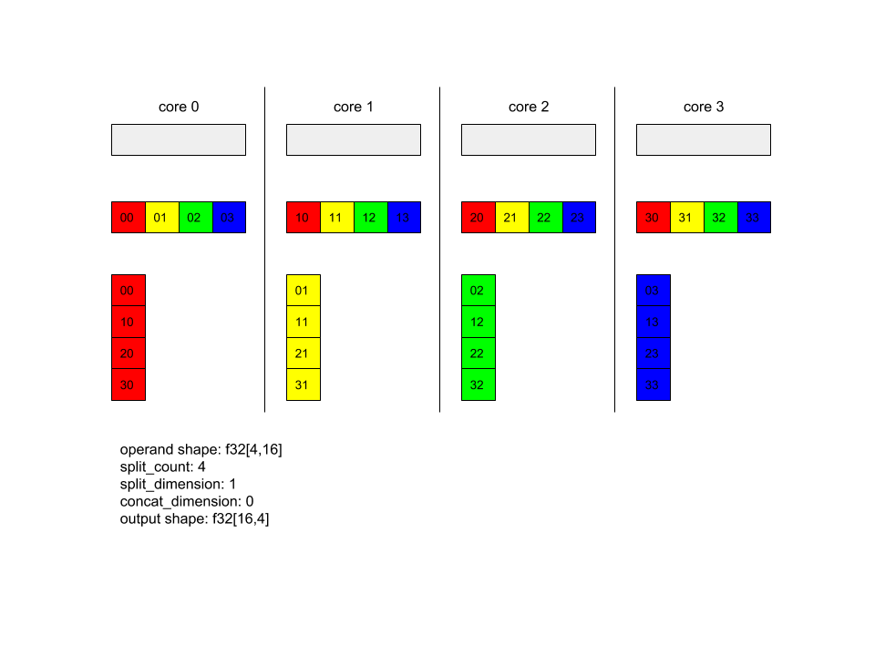
In questo esempio, ci sono 4 core che partecipano a Alltoall. Su ciascun nucleo, l'operando è suddiviso in 4 parti lungo la dimensione 0, quindi ogni parte ha la forma f32[4,4]. Le quattro parti sono sparse per tutti i core. Poi ogni core concatena le parti ricevute lungo la dimensione 1, seguendo l'ordine del core 0-4. Quindi l'output su ciascun core ha la forma f32[16,4].
BatchNormGrad
Consulta anche
XlaBuilder::BatchNormGrad
e il documento originale sulla normalizzazione dei batch
per una descrizione dettagliata dell'algoritmo.
Calcola i gradienti della norma batch.
BatchNormGrad(operand, scale, mean, variance, grad_output, epsilon, feature_index)
| Argomenti | Tipo | Semantica |
|---|---|---|
operand |
XlaOp |
n matrice dimensionale da normalizzare (x) |
scale |
XlaOp |
Matrice monodimensionale (\(\gamma\)) |
mean |
XlaOp |
Matrice monodimensionale (\(\mu\)) |
variance |
XlaOp |
Matrice monodimensionale (\(\sigma^2\)) |
grad_output |
XlaOp |
Gradienti passati a BatchNormTraining (\(\nabla y\)) |
epsilon |
float |
Valore Epsilon (\(\epsilon\)) |
feature_index |
int64 |
Indice alla dimensione Funzionalità in operand |
Per ogni elemento nella dimensione elemento (feature_index è l'indice per la dimensione elemento in operand), l'operazione calcola i gradienti rispetto a operand, offset e scale in tutte le altre dimensioni. feature_index deve essere un indice valido per la dimensione della funzionalità in operand.
I tre gradienti sono definiti dalle seguenti formule (supponendo che un array tridimensionale sia operand e con l'indice delle dimensioni delle caratteristiche l, le dimensioni del batch m e le dimensioni spaziali w e h):
\[ \begin{split} c_l&= \frac{1}{mwh}\sum_{i=1}^m\sum_{j=1}^w\sum_{k=1}^h \left( \nabla y_{ijkl} \frac{x_{ijkl} - \mu_l}{\sigma^2_l+\epsilon} \right) \\\\ d_l&= \frac{1}{mwh}\sum_{i=1}^m\sum_{j=1}^w\sum_{k=1}^h \nabla y_{ijkl} \\\\ \nabla x_{ijkl} &= \frac{\gamma_{l} }{\sqrt{\sigma^2_{l}+\epsilon} } \left( \nabla y_{ijkl} - d_l - c_l (x_{ijkl} - \mu_{l}) \right) \\\\ \nabla \gamma_l &= \sum_{i=1}^m\sum_{j=1}^w\sum_{k=1}^h \left( \nabla y_{ijkl} \frac{x_{ijkl} - \mu_l}{\sqrt{\sigma^2_{l}+\epsilon} } \right) \\\\\ \nabla \beta_l &= \sum_{i=1}^m\sum_{j=1}^w\sum_{k=1}^h \nabla y_{ijkl} \end{split} \]
Gli input mean e variance rappresentano i valori dei momenti nelle dimensioni batch e spaziali.
Il tipo di output è una tupla di tre handle:
| Output | Tipo | Semantica |
|---|---|---|
grad_operand
|
XlaOp
|
gradiente rispetto all'input operand ($\nabla
x$) |
grad_scale
|
XlaOp
|
gradiente rispetto all'input scale ($\nabla
\gamma$) |
grad_offset
|
XlaOp
|
gradiente rispetto all'input offset($\nabla
\beta$) |
BatchNormInference
Consulta anche
XlaBuilder::BatchNormInference
e il documento originale sulla normalizzazione dei batch
per una descrizione dettagliata dell'algoritmo.
Normalizza un array per dimensioni batch e spaziali.
BatchNormInference(operand, scale, offset, mean, variance, epsilon, feature_index)
| Argomenti | Tipo | Semantica |
|---|---|---|
operand |
XlaOp |
n array dimensionale da normalizzare |
scale |
XlaOp |
matrice monodimensionale |
offset |
XlaOp |
matrice monodimensionale |
mean |
XlaOp |
matrice monodimensionale |
variance |
XlaOp |
matrice monodimensionale |
epsilon |
float |
Valore Epsilon |
feature_index |
int64 |
Indice alla dimensione Funzionalità in operand |
Per ogni caratteristica nella dimensione caratteristica (feature_index è l'indice per la dimensione elemento in operand), l'operazione calcola la media e la varianza tra tutte le altre dimensioni e utilizza la media e la varianza per normalizzare ciascun elemento in operand. feature_index deve essere un indice valido per la dimensione caratteristica in operand.
BatchNormInference equivale a chiamare BatchNormTraining senza calcolare mean e variance per ogni batch. Utilizza invece gli input mean e variance come valori stimati. Lo scopo di questa operazione è ridurre la latenza nell'inferenza, da cui il nome BatchNormInference.
L'output è un array normalizzato n-dimensionale con la stessa forma dell'input
operand.
BatchNormTraining
Vedi anche
XlaBuilder::BatchNormTraining
e the original batch normalization paper
per una descrizione dettagliata dell'algoritmo.
Normalizza un array per dimensioni batch e spaziali.
BatchNormTraining(operand, scale, offset, epsilon, feature_index)
| Argomenti | Tipo | Semantica |
|---|---|---|
operand |
XlaOp |
n matrice dimensionale da normalizzare (x) |
scale |
XlaOp |
Matrice monodimensionale (\(\gamma\)) |
offset |
XlaOp |
Matrice monodimensionale (\(\beta\)) |
epsilon |
float |
Valore Epsilon (\(\epsilon\)) |
feature_index |
int64 |
Indice alla dimensione Funzionalità in operand |
Per ogni caratteristica nella dimensione caratteristica (feature_index è l'indice per la dimensione elemento in operand), l'operazione calcola la media e la varianza tra tutte le altre dimensioni e utilizza la media e la varianza per normalizzare ciascun elemento in operand. feature_index deve essere un indice valido per la dimensione caratteristica in operand.
L'algoritmo funziona nel seguente modo per ogni batch in operand \(x\) contenente elementi m con w e h come dimensione delle dimensioni spaziali (supponendo che operand sia un array 4 dimensioni):
Calcola la media batch \(\mu_l\) per ogni caratteristica
lnella dimensione caratteristica: \(\mu_l=\frac{1}{mwh}\sum_{i=1}^m\sum_{j=1}^w\sum_{k=1}^h x_{ijkl}\)Calcola la varianza batch \(\sigma^2_l\): $\sigma^2l=\frac{1}{mwh}\sum{i=1}^m\sum{j=1}^w\sum{k=1}^h (x_{ijkl} - \mu_l)^2$
Normalizza, ridimensiona e sposta: \(y_{ijkl}=\frac{\gamma_l(x_{ijkl}-\mu_l)}{\sqrt[2]{\sigma^2_l+\epsilon} }+\beta_l\)
Il valore epsilon, di solito un numero piccolo, viene aggiunto per evitare errori di divisione per zero.
Il tipo di output è una tupla di tre XlaOp:
| Output | Tipo | Semantica |
|---|---|---|
output
|
XlaOp
|
n matrice dimensionale con la stessa forma dell'input
operand (y) |
batch_mean |
XlaOp |
Matrice monodimensionale (\(\mu\)) |
batch_var |
XlaOp |
Matrice monodimensionale (\(\sigma^2\)) |
batch_mean e batch_var sono momenti calcolati nelle dimensioni spaziali e batch utilizzando le formule precedenti.
BitcastConvertType
Vedi anche
XlaBuilder::BitcastConvertType.
Analogamente a tf.bitcast in TensorFlow, esegue un'operazione bitcast a livello di elemento da una forma di dati a una forma di destinazione. Le dimensioni di input e output devono
corrispondere: ad esempio, gli elementi s32 diventano elementi f32 tramite la routine bitcast e un
elemento s32 diventerà quattro elementi s8. Bitcast viene implementato come cast di basso livello, quindi macchine con rappresentazioni in virgola mobile diverse daranno risultati diversi.
BitcastConvertType(operand, new_element_type)
| Argomenti | Tipo | Semantica |
|---|---|---|
operand |
XlaOp |
array di tipo T con dims D |
new_element_type |
PrimitiveType |
tipo U |
Le dimensioni dell'operando e della forma di destinazione devono corrispondere, a parte l'ultima dimensione che cambierà in base al rapporto delle dimensioni primitive prima e dopo la conversione.
I tipi di elementi di origine e di destinazione non devono essere tuple.
Conversione di bitcast in tipo primitivo di larghezza diversa
BitcastConvert L'istruzione HLO supporta il caso in cui le dimensioni del tipo di elemento di output T' non corrispondano alle dimensioni dell'elemento di input T. Poiché
l'intera operazione è concettualmente un bitcast e non modifica i byte sottostanti, la forma dell'elemento di output deve cambiare. Per B = sizeof(T), B' =
sizeof(T'), ci sono due casi possibili.
Innanzitutto, quando B > B', la forma di output riceve una nuova dimensione minore della dimensione B/B'. Ad esempio:
f16[10,2]{1,0} %output = f16[10,2]{1,0} bitcast-convert(f32[10]{0} %input)
La regola rimane la stessa per i valori scalari efficaci:
f16[2]{0} %output = f16[2]{0} bitcast-convert(f32[] %input)
In alternativa, per B' > B l'istruzione richiede che l'ultima dimensione logica
della forma di input sia uguale a B'/B, e questa dimensione viene eliminata durante
la conversione:
f32[10]{0} %output = f32[10]{0} bitcast-convert(f16[10,2]{1,0} %input)
Tieni presente che le conversioni tra larghezze di bit diverse non sono a livello di elemento.
Trasmetti un annuncio
Vedi anche
XlaBuilder::Broadcast.
Aggiunge dimensioni a un array duplicando i dati al suo interno.
Broadcast(operand, broadcast_sizes)
| Argomenti | Tipo | Semantica |
|---|---|---|
operand |
XlaOp |
L'array da duplicare |
broadcast_sizes |
ArraySlice<int64> |
Le dimensioni delle nuove dimensioni |
Le nuove dimensioni vengono inserite a sinistra, ad esempio se broadcast_sizes ha
valori {a0, ..., aN} e la forma dell'operando ha dimensioni {b0, ..., bM},
la forma dell'output ha dimensioni {a0, ..., aN, b0, ..., bM}.
Le nuove dimensioni vengono indicizzate in copie dell'operando, ad esempio
output[i0, ..., iN, j0, ..., jM] = operand[j0, ..., jM]
Ad esempio, se operand è un f32 scalare con valore 2.0f e
broadcast_sizes è {2, 3}, il risultato sarà un array con forma
f32[2, 3] e tutti i valori nel risultato saranno 2.0f.
BroadcastInDim
Vedi anche
XlaBuilder::BroadcastInDim.
Espande le dimensioni e il ranking di un array duplicando i dati al suo interno.
BroadcastInDim(operand, out_dim_size, broadcast_dimensions)
| Argomenti | Tipo | Semantica |
|---|---|---|
operand |
XlaOp |
L'array da duplicare |
out_dim_size |
ArraySlice<int64> |
Le dimensioni delle dimensioni della forma di destinazione |
broadcast_dimensions |
ArraySlice<int64> |
A quale dimensione nella forma di target corrisponde ciascuna dimensione della forma dell'operando |
Simile a Broadcast, ma consente di aggiungere dimensioni ovunque ed espandere le dimensioni esistenti con la dimensione 1.
operand viene trasmesso nella forma descritta da out_dim_size.
broadcast_dimensions mappa le dimensioni di operand con le dimensioni
della forma di destinazione, ad esempio la dimensione i'esima dell'operando è mappata alla dimensione
broadcast_dimension[i]'esima della forma di output. Le dimensioni di operand devono avere dimensione 1 o avere le stesse dimensioni della dimensione nella forma di output a cui sono mappate. Le altre dimensioni vengono riempite
con dimensioni di 1. La trasmissione con dimensioni degenerate quindi trasmette in queste dimensioni degenerate per raggiungere la forma di output. La semantica è descritta in dettaglio nella pagina di trasmissione.
Call
Vedi anche
XlaBuilder::Call.
Avvia un calcolo con gli argomenti specificati.
Call(computation, args...)
| Argomenti | Tipo | Semantica |
|---|---|---|
computation |
XlaComputation |
calcolo di tipo T_0, T_1, ..., T_{N-1} -> S con N parametri di tipo arbitrario |
args |
sequenza di N XlaOp |
N argomenti di tipo arbitrario |
L'arità e i tipi di args devono corrispondere ai parametri di
computation. Non può avere args.
Cholesky
Vedi anche
XlaBuilder::Cholesky.
Calcola la scomposizione di Cholesky di un gruppo di matrici definite positive simmetriche (ermitiane).
Cholesky(a, lower)
| Argomenti | Tipo | Semantica |
|---|---|---|
a |
XlaOp |
un array con rango > 2 di tipo complesso o con virgola mobile. |
lower |
bool |
se utilizzare il triangolo superiore o inferiore di a. |
Se lower è true, calcola le matrici triangolari inferiori l in modo che $a = l .
l^T$. Se lower è false, calcola le matrici triangolari superiori u in modo che
\(a = u^T . u\).
I dati di input vengono letti solo dal triangolo inferiore/superiore di a, a seconda del
valore di lower. I valori dell'altro triangolo vengono ignorati. I dati di output vengono restituiti nello stesso triangolo; i valori nell'altro triangolo sono definiti dall'implementazione e possono essere qualsiasi cosa.
Se il ranking di a è maggiore di 2, a viene trattato come un gruppo di matrici, dove tutte le dimensioni tranne le due dimensioni secondarie sono dimensioni batch.
Se a non è una definizione positiva simmetrica (hermitiana), il risultato è definito dall'implementazione.
Con morsetto
Vedi anche
XlaBuilder::Clamp.
Blocca un operando che rientra nell'intervallo compreso tra un valore minimo e un valore massimo.
Clamp(min, operand, max)
| Argomenti | Tipo | Semantica |
|---|---|---|
min |
XlaOp |
array di tipo T |
operand |
XlaOp |
array di tipo T |
max |
XlaOp |
array di tipo T |
Dati un operando e i valori minimo e massimo, restituisce l'operando se è compreso nell'intervallo compreso tra il minimo e il massimo, altrimenti restituisce il valore minimo se l'operando è inferiore a questo intervallo o il valore massimo se l'operando è superiore a questo intervallo. Vale a dire, clamp(a, x, b) = min(max(a, x), b).
Tutte e tre le matrici devono avere la stessa forma. In alternativa, come forma limitata di
trasmissione, min e/o max possono essere un tipo scalare di tipo T.
Esempio con min e max scalari:
let operand: s32[3] = {-1, 5, 9};
let min: s32 = 0;
let max: s32 = 6;
==>
Clamp(min, operand, max) = s32[3]{0, 5, 6};
Comprimi
Vedi anche
XlaBuilder::Collapse
e l'operazione tf.reshape.
Comprime le dimensioni di un array in un'unica dimensione.
Collapse(operand, dimensions)
| Argomenti | Tipo | Semantica |
|---|---|---|
operand |
XlaOp |
array di tipo T |
dimensions |
int64 vettore |
sottoinsieme consecutivo di dimensioni T in ordine. |
La compressione sostituisce il sottoinsieme specificato di dimensioni dell'operando con un'unica dimensione. Gli argomenti di input sono un array arbitrario di tipo T e un vettore costante di tempo di compilazione degli indici di dimensione. Gli indici delle dimensioni devono essere un sottoinsieme consecutivo di dimensioni T in ordine (numeri di dimensione da bassi ad alti). Pertanto, {0, 1, 2}, {0, 1} o {1, 2} sono tutti insiemi di dimensioni validi, al contrario di {1, 0} o {0, 2}. che vengono sostituite da un'unica nuova dimensione, nella stessa posizione nella sequenza di dimensioni di quelle da sostituire, con la nuova dimensione uguale al prodotto delle dimensioni originali. Il numero di dimensione più basso in dimensions è la dimensione a variazione più lenta (la più importante) nella nidificazione del loop che comprime queste dimensioni, mentre il numero di dimensione più alto varia in modo più rapido (la più minima). Consulta l'operatore tf.reshape se è necessario un ordine di compressione più generale.
Ad esempio, supponiamo che v sia un array di 24 elementi:
let v = f32[4x2x3] { { {10, 11, 12},  {15, 16, 17} },
{ {20, 21, 22},  {25, 26, 27} },
{ {30, 31, 32},  {35, 36, 37} },
{ {40, 41, 42},  {45, 46, 47} } };

// Collapse to a single dimension, leaving one dimension.
let v012 = Collapse(v, {0,1,2});
then v012 == f32[24] {10, 11, 12, 15, 16, 17,
20, 21, 22, 25, 26, 27,
30, 31, 32, 35, 36, 37,
40, 41, 42, 45, 46, 47};

// Collapse the two lower dimensions, leaving two dimensions.
let v01 = Collapse(v, {0,1});
then v01 == f32[4x6] { {10, 11, 12, 15, 16, 17},
{20, 21, 22, 25, 26, 27},
{30, 31, 32, 35, 36, 37},
{40, 41, 42, 45, 46, 47} };

// Collapse the two higher dimensions, leaving two dimensions.
let v12 = Collapse(v, {1,2});
then v12 == f32[8x3] { {10, 11, 12},
{15, 16, 17},
{20, 21, 22},
{25, 26, 27},
{30, 31, 32},
{35, 36, 37},
{40, 41, 42},
{45, 46, 47} };
CollectivePermute
Vedi anche
XlaBuilder::CollectivePermute.
CollectivePermute è un'operazione collettiva che invia e riceve repliche incrociate di dati.
CollectivePermute(operand, source_target_pairs)
| Argomenti | Tipo | Semantica |
|---|---|---|
operand |
XlaOp |
n array di input dimensionale |
source_target_pairs |
<int64, int64> vettore |
Un elenco di coppie (source_replica_id, target_replica_id). Per ogni coppia, l'operando viene inviato dalla replica di origine a quella di destinazione. |
Tieni presente che su source_target_pair sono previste le seguenti limitazioni:
- Due coppie qualsiasi non devono avere lo stesso ID replica di destinazione e non devono avere lo stesso ID replica di origine.
- Se un ID replica non è un target in nessuna coppia, l'output su quella replica è un tensore composto da zero con la stessa forma dell'input.
Concatena
Vedi anche
XlaBuilder::ConcatInDim.
Concatena compone un array da più operandi di array. L'array ha la stessa posizione di ciascuno degli operandi dell'array di input (che devono avere lo stesso ranking l'uno dell'altro) e contiene gli argomenti nell'ordine in cui sono stati specificati.
Concatenate(operands..., dimension)
| Argomenti | Tipo | Semantica |
|---|---|---|
operands |
sequenza di N XlaOp |
Matrici N di tipo T con dimensioni [L0, L1, ...]. Richiede N >= 1. |
dimension |
int64 |
Un valore nell'intervallo [0, N) che indica la dimensione da concatenare tra operands. |
Ad eccezione di dimension, tutte le dimensioni devono essere uguali. Questo perché XLA non supporta array "irregolari". Nota inoltre che i valori di rango 0 non possono essere concatenati (poiché è impossibile assegnare un nome alla dimensione lungo la quale avviene la concatenazione).
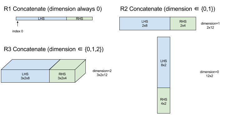
Esempio unidimensionale:
Concat({ {2, 3}, {4, 5}, {6, 7} }, 0)
>>> {2, 3, 4, 5, 6, 7}
Esempio bidimensionale:
let a = {
{1, 2},
{3, 4},
{5, 6},
};
let b = {
{7, 8},
};
Concat({a, b}, 0)
>>> {
{1, 2},
{3, 4},
{5, 6},
{7, 8},
}
Diagramma:
Condizionali
Vedi anche
XlaBuilder::Conditional.
Conditional(pred, true_operand, true_computation, false_operand,
false_computation)
| Argomenti | Tipo | Semantica |
|---|---|---|
pred |
XlaOp |
Scalare di tipo PRED |
true_operand |
XlaOp |
Argomento di tipo \(T_0\) |
true_computation |
XlaComputation |
XlaComputation di tipo \(T_0 \to S\) |
false_operand |
XlaOp |
Argomento di tipo \(T_1\) |
false_computation |
XlaComputation |
XlaComputation di tipo \(T_1 \to S\) |
Esegue true_computation se pred è true, false_computation se pred è false e restituisce il risultato.
true_computation deve contenere un singolo argomento di tipo \(T_0\) e verrà richiamato con true_operand, che deve essere dello stesso tipo. false_computation deve includere un singolo argomento di tipo \(T_1\) e verrà richiamato con false_operand, che deve essere dello stesso tipo. Il tipo del valore restituito di true_computation e false_computation deve essere lo stesso.
Tieni presente che verrà eseguito un solo tipo tra true_computation e false_computation a seconda del valore di pred.
Conditional(branch_index, branch_computations, branch_operands)
| Argomenti | Tipo | Semantica |
|---|---|---|
branch_index |
XlaOp |
Scalare di tipo S32 |
branch_computations |
sequenza di N XlaComputation |
XlaComputations di tipo \(T_0 \to S , T_1 \to S , ..., T_{N-1} \to S\) |
branch_operands |
sequenza di N XlaOp |
Argomenti di tipo \(T_0 , T_1 , ..., T_{N-1}\) |
Esegue branch_computations[branch_index] e restituisce il risultato. Se branch_index è un S32 < 0 o >= N, branch_computations[N-1] viene eseguito come ramo predefinito.
Ogni branch_computations[b] deve contenere un singolo argomento di tipo \(T_b\) e verrà richiamato con branch_operands[b], che deve essere dello stesso tipo. Il
tipo di valore restituito per ogni branch_computations[b] deve essere lo stesso.
Tieni presente che verrà eseguito solo uno dei branch_computations a seconda del valore di branch_index.
Conv. (convoluzione)
Vedi anche
XlaBuilder::Conv.
Come ConvWithGeneralPadding, ma la spaziatura interna viene specificata brevemente come SAME o VALID. La STESSA spaziatura interna riempie l'input (lhs) con zeri, in modo che l'output abbia la stessa forma dell'input quando non si tiene conto dell'intervallo. Spaziatura interna VALIDA significa semplicemente che non è presente alcuna spaziatura interna.
ConvWithGeneralPadding (convolution)
Vedi anche
XlaBuilder::ConvWithGeneralPadding.
Calcola una convoluzione del tipo utilizzato nelle reti neurali. In questo caso, una convoluzione può essere considerata come una finestra n-dimensionale che si sposta su un'area di base n-dimensionale e viene eseguito un calcolo per ogni possibile posizione della finestra.
| Argomenti | Tipo | Semantica |
|---|---|---|
lhs |
XlaOp |
classifica n+2 array di input |
rhs |
XlaOp |
rango n+2 array di pesi del kernel |
window_strides |
ArraySlice<int64> |
Array n-d di passi del kernel |
padding |
ArraySlice< pair<int64,int64>> |
array n-d di spaziatura interna (bassa, alta) |
lhs_dilation |
ArraySlice<int64> |
Array del fattore di dilatazione n-d lhs |
rhs_dilation |
ArraySlice<int64> |
Array del fattore di dilatazione rhs n-d |
feature_group_count |
int64 | il numero di gruppi di funzionalità |
batch_group_count |
int64 | il numero di gruppi in batch |
Sia n il numero di dimensioni spaziali. L'argomento lhs è un array di rango n+2 che descrive l'area di base. Questo è chiamato input, anche se ovviamente
la destra è anche un input. In una rete neurale, queste sono le attivazioni dell'input.
Le dimensioni n+2 sono, nel seguente ordine:
batch: ogni coordinata in questa dimensione rappresenta un input indipendente per cui viene eseguita la convoluzione.z/depth/features: a ogni posizione (y,x) nell'area di base è associato un vettore che rientra in questa dimensione.spatial_dims: descrive le dimensioni spazialinche definiscono l'area di base attraverso cui si sposta la finestra.
L'argomento rhs è un array di rango n+2 che descrive il filtro/kernel/finestra convoluzionale. Le dimensioni sono, nel seguente ordine:
output-z: la dimensionezdell'output.input-z: la dimensione di questa dimensione moltiplicata perfeature_group_countdeve corrispondere alla dimensione della dimensionezin lh.spatial_dims: descrive le dimensioni spazialinche definiscono la finestra n-d che si sposta lungo l'area di base.
L'argomento window_strides specifica il passo della finestra convoluzionale nelle dimensioni spaziali. Ad esempio, se l'intervallo nella prima dimensione spaziale è 3, la finestra può essere posizionata solo nelle coordinate in cui il primo indice spaziale è divisibile per 3.
L'argomento padding specifica la quantità di spaziatura interna pari a zero da applicare all'area di base. La quantità di spaziatura interna può essere negativa: il valore assoluto di spaziatura negativa indica il numero di elementi da rimuovere dalla dimensione specificata prima di eseguire la convoluzione. padding[0] specifica la spaziatura interna per la dimensione y, mentre padding[1] specifica la spaziatura interna per la dimensione x. Ogni
coppia ha la spaziatura interna bassa come primo elemento e la spaziatura interna alta come secondo
elemento. La spaziatura interna bassa viene applicata nella direzione degli indici più bassi, mentre la spaziatura interna elevata viene applicata nella direzione degli indici più alti. Ad esempio, se padding[1] è (2,3), ci sarà una spaziatura interna di 2 zeri a sinistra e di 3 zeri a destra nella seconda dimensione spaziale. L'utilizzo della spaziatura interna equivale
all'inserimento degli stessi valori zero nell'input (lhs) prima
di eseguire la convoluzione.
Gli argomenti lhs_dilation e rhs_dilation specificano il fattore di dilatazione da
applicare rispettivamente a lhs e rhs, in ogni dimensione spaziale. Se il fattore di dilatazione in una dimensione spaziale è d, i fori d-1 vengono implicitamente posizionati tra ciascuna voce in quella dimensione, aumentando le dimensioni dell'array. I fori vengono riempiti con un valore autonomo, che per convoluzione significa
zeri.
La dilatazione della parte destra è anche chiamata convoluzione atrosa. Per maggiori dettagli, consulta
tf.nn.atrous_conv2d. La dilatazione degli lhs è anche detta
convoluzione trasposta. Per maggiori dettagli, vedi tf.nn.conv2d_transpose.
L'argomento feature_group_count (valore predefinito 1) può essere utilizzato per le convoluzioni raggruppate. feature_group_count deve essere un divisore sia della dimensione della funzionalità di input
che della dimensione della funzionalità di output. Se feature_group_count è maggiore di 1, significa che concettualmente la dimensione caratteristica di input e output e la dimensione caratteristica di output rhs sono suddivise uniformemente in molti gruppi feature_group_count, ogni gruppo è costituito da una sottosequenza di caratteristiche consecutive. La dimensione della funzionalità di input rhs deve essere uguale alla dimensione della funzionalità di input di lhs divisa per feature_group_count (quindi ha già le dimensioni di un gruppo di funzionalità di input). I gruppi i-esima vengono utilizzati insieme per calcolare
feature_group_count per molte convoluzioni separate. I risultati di queste convoluzioni sono concatenati nella dimensione delle caratteristiche di output.
Per la convoluzione in profondità, l'argomento feature_group_count viene impostato sulla
dimensione della funzionalità di input e il filtro viene rimodellato da
[filter_height, filter_width, in_channels, channel_multiplier] a
[filter_height, filter_width, 1, in_channels * channel_multiplier]. Per maggiori
dettagli, consulta tf.nn.depthwise_conv2d.
L'argomento batch_group_count (valore predefinito 1) può essere utilizzato per i filtri raggruppati durante la retropropagazione dell'errore. batch_group_count deve essere un divisore della
dimensione batch lhs (input). Se batch_group_count è maggiore
di 1, significa che la dimensione batch di output deve avere una dimensione input batch
/ batch_group_count. batch_group_count deve essere un divisore della dimensione della funzionalità di output.
La forma di output ha queste dimensioni, nel seguente ordine:
batch: la dimensione di questa dimensione moltiplicata perbatch_group_countdeve corrispondere alla dimensione della dimensionebatchnei caratteri lh.z: ha le stesse dimensioni dioutput-zsul kernel (rhs).spatial_dims: un valore per ogni posizionamento valido della finestra convoluzionale.

La figura sopra mostra il funzionamento del campo batch_group_count. In modo efficace, suddividiamo ogni batch lhs in gruppi batch_group_count e facciamo lo stesso per le funzionalità di output. Quindi, per ognuno di questi gruppi eseguiamo convoluzioni a coppie e concateniamo l'output lungo la dimensione della caratteristica di output. La semantica operativa di tutte le altre dimensioni (funzionalità e spaziale) rimane la stessa.
I posizionamenti validi della finestra convoluzionale sono determinati dai passi e dalle dimensioni dell'area di base dopo la spaziatura interna.
Per descrivere la funzione di una convoluzione, considera una convoluzione 2d e scegli nell'output alcune coordinate batch, z, y e x fisse. Poi (y,x) è la posizione di un angolo della finestra all'interno dell'area della base (ad esempio l'angolo in alto a sinistra, a seconda di come interpreti le dimensioni spaziali). Ora abbiamo una finestra 2D, presa dall'area di base, in cui ogni punto 2D è associato a un vettore 1d, quindi otteniamo un riquadro 3D. Dal kernel convoluzionale, dato che abbiamo corretto la coordinata di output z, abbiamo anche un 3d box. Le due caselle hanno le stesse dimensioni, quindi possiamo prendere la somma dei prodotti a livello di elemento tra i due riquadri (in modo simile a un prodotto scalare). Questo è il valore di output.
Tieni presente che, se output-z è, ad esempio, 5, ogni posizione della finestra produce 5
valori nell'output nella dimensione z dell'output. Questi valori variano
in quale parte del kernel convoluzionale viene utilizzata: esiste un riquadro 3D separato di valori
utilizzato per ogni coordinata output-z. Questo può essere paragonato a cinque convoluzioni
distinte con un filtro diverso per ognuna.
Ecco lo pseudo-codice per una convoluzione 2D con spaziatura interna e passo:
for (b, oz, oy, ox) {  // output coordinates
  value = 0;
  for (iz, ky, kx) {  // kernel coordinates and input z
    iy = oy*stride_y + ky - pad_low_y;
    ix = ox*stride_x + kx - pad_low_x;
    if ((iy, ix) inside the base area considered without padding) {
      value += input(b, iz, iy, ix) * kernel(oz, iz, ky, kx);
    }
  }
  output(b, oz, oy, ox) = value;
}
ConvertElementType
Vedi anche
XlaBuilder::ConvertElementType.
Simile a static_cast a livello di elemento in C++, esegue un'operazione di conversione a livello di elemento da una forma di dati a una forma di destinazione. Le dimensioni devono
corrispondere e la conversione è basata sugli elementi; ad esempio, gli elementi s32 diventano
elementi f32 tramite una routine di conversione da s32 a f32.
ConvertElementType(operand, new_element_type)
| Argomenti | Tipo | Semantica |
|---|---|---|
operand |
XlaOp |
array di tipo T con dims D |
new_element_type |
PrimitiveType |
tipo U |
Le dimensioni dell'operando e la forma di destinazione devono corrispondere. I tipi di elementi di origine e di destinazione non devono essere tuple.
Una conversione come T=s32 in U=f32 eseguirà una routine di conversione da int a virgola mobile di normalizzazione, come il arrotondamento al più vicino pari.
let a: s32[3] = {0, 1, 2};
let b: f32[3] = convert(a, f32);
then b == f32[3]{0.0, 1.0, 2.0}
CrossReplicaSum
Esegue AllReduce con un calcolo di somma.
CustomCall
Vedi anche
XlaBuilder::CustomCall.
Richiama una funzione fornita dall'utente all'interno di un calcolo.
CustomCall(target_name, args..., shape)
| Argomenti | Tipo | Semantica |
|---|---|---|
target_name |
string |
Nome della funzione. Verrà emessa un'istruzione di chiamata che ha come target il nome di questo simbolo. |
args |
sequenza di N XlaOp |
N argomenti di tipo arbitrario, che verranno passati alla funzione. |
shape |
Shape |
Forma di output della funzione |
La firma della funzione è la stessa, indipendentemente dall'arità o dal tipo di argomenti:
extern "C" void target_name(void* out, void** in);
Ad esempio, se CustomCall viene utilizzata come segue:
let x = f32[2] {1,2};
let y = f32[2x3] { {10, 20, 30}, {40, 50, 60} };

CustomCall("myfunc", {x, y}, f32[3x3])
Ecco un esempio di implementazione di myfunc:
extern "C" void myfunc(void* out, void** in) {
  float (&x)[2] = *static_cast<float(*)[2]>(in[0]);
  float (&y)[2][3] = *static_cast<float(*)[2][3]>(in[1]);
  EXPECT_EQ(1, x[0]);
  EXPECT_EQ(2, x[1]);
  EXPECT_EQ(10, y[0][0]);
  EXPECT_EQ(20, y[0][1]);
  EXPECT_EQ(30, y[0][2]);
  EXPECT_EQ(40, y[1][0]);
  EXPECT_EQ(50, y[1][1]);
  EXPECT_EQ(60, y[1][2]);
  float (&z)[3][3] = *static_cast<float(*)[3][3]>(out);
  z[0][0] = x[1] + y[1][0];
  // ...
}
La funzione fornita dall'utente non deve avere effetti collaterali e la sua esecuzione deve essere idempotente.
Punto
Vedi anche
XlaBuilder::Dot.
Dot(lhs, rhs)
| Argomenti | Tipo | Semantica |
|---|---|---|
lhs |
XlaOp |
array di tipo T |
rhs |
XlaOp |
array di tipo T |
La semantica esatta di questa operazione dipende dai ranghi degli operandi:
| Input | Output | Semantica |
|---|---|---|
vettore [n] dot vettore [n] |
scalare | prodotto Vector Dot |
matrice [m x k] dot vettore [k] |
vettore [m] | moltiplicazione matriciale-vettori |
matrice [m x k] dot matrice [k x n] |
matrice [m x n] | moltiplicazione matriciale-matrici |
L'operazione esegue la somma dei prodotti per la seconda dimensione di lhs (o
la prima se ha ranking 1) e la prima dimensione di rhs. Queste sono le
dimensioni "contrattate". Le dimensioni contrattate di lhs e rhs devono avere
le stesse dimensioni. In pratica, può essere utilizzata per eseguire prodotti scalare tra vettori, moltiplicazioni di vettore/matrici o moltiplicazioni di matrici/matrici.
DotGeneral
Vedi anche
XlaBuilder::DotGeneral.
DotGeneral(lhs, rhs, dimension_numbers)
| Argomenti | Tipo | Semantica |
|---|---|---|
lhs |
XlaOp |
array di tipo T |
rhs |
XlaOp |
array di tipo T |
dimension_numbers |
DotDimensionNumbers |
numeri di dimensioni contrattuali e batch |
Simile al punto, ma consente di specificare numeri di dimensioni contrattuali e batch per lhs e rhs.
| Campi DotDimensionNumbers | Tipo | Semantica |
|---|---|---|
lhs_contracting_dimensions
|
int64 ripetuto | lhs numeri di dimensioni
contraenti |
rhs_contracting_dimensions
|
int64 ripetuto | rhs numeri di dimensioni
contraenti |
lhs_batch_dimensions
|
int64 ripetuto | lhs numeri di dimensioni batch |
rhs_batch_dimensions
|
int64 ripetuto | rhs numeri di dimensioni batch |
DotGeneral esegue la somma dei prodotti rispetto alle dimensioni contrattuali specificate in
dimension_numbers.
I numeri delle dimensioni contrattuali associate di lhs e rhs non devono essere uguali, ma devono avere le stesse dimensioni.
Esempio con i numeri delle dimensioni contrattuali:
lhs = { {1.0, 2.0, 3.0},
{4.0, 5.0, 6.0} }

rhs = { {1.0, 1.0, 1.0},
{2.0, 2.0, 2.0} }

DotDimensionNumbers dnums;
dnums.add_lhs_contracting_dimensions(1);
dnums.add_rhs_contracting_dimensions(1);

DotGeneral(lhs, rhs, dnums) -> { {6.0, 12.0},
{15.0, 30.0} }
I numeri delle dimensioni batch associati da lhs e rhs devono avere le stesse dimensioni.
Esempio con numeri di dimensioni batch (matrici dimensione batch 2, matrici 2x2):
lhs = { { {1.0, 2.0},
{3.0, 4.0} },
{ {5.0, 6.0},
{7.0, 8.0} } }

rhs = { { {1.0, 0.0},
{0.0, 1.0} },
{ {1.0, 0.0},
{0.0, 1.0} } }

DotDimensionNumbers dnums;
dnums.add_lhs_contracting_dimensions(2);
dnums.add_rhs_contracting_dimensions(1);
dnums.add_lhs_batch_dimensions(0);
dnums.add_rhs_batch_dimensions(0);

DotGeneral(lhs, rhs, dnums) -> { { {1.0, 2.0},
{3.0, 4.0} },
{ {5.0, 6.0},
{7.0, 8.0} } }
| Input | Output | Semantica |
|---|---|---|
[b0, m, k] dot [b0, k, n] |
[b0, m, n] | matmul batch |
[b0, b1, m, k] dot [b0, b1, k, n] |
[b0, b1, m, n] | matmul batch |
Ne consegue che il numero di dimensione risultante inizia con la dimensione batch, poi la dimensione senza contratto/non batch lhs e infine la dimensione senza contratto/non batch rhs.
DynamicSlice
Vedi anche
XlaBuilder::DynamicSlice.
DynamicSlice estrae un sottoarray dall'array di input nel livello dinamico start_indices. La dimensione della sezione in ogni dimensione viene passata in size_indices, che specifica il punto finale degli intervalli di sezioni esclusive in ogni dimensione: [inizio, inizio + dimensione). La forma di start_indices deve avere ranking ==
1, con dimensioni della dimensione uguali al rango di operand.
DynamicSlice(operand, start_indices, size_indices)
| Argomenti | Tipo | Semantica |
|---|---|---|
operand |
XlaOp |
Matrice dimensionale N di tipo T |
start_indices |
sequenza di N XlaOp |
Elenco di N numeri interi scalari contenenti gli indici iniziali della sezione per ogni dimensione. Il valore deve essere maggiore o uguale a zero. |
size_indices |
ArraySlice<int64> |
Elenco di N numeri interi contenenti la dimensione della sezione per ogni dimensione. Ogni valore deve essere rigorosamente maggiore di zero e la dimensione inizio + deve essere minore o uguale alla dimensione della dimensione per evitare di includere le dimensioni della dimensione del modulo. |
Gli indici di sezione effettivi vengono calcolati applicando la seguente trasformazione per ogni indice i in [1, N) prima di eseguire la sezione:
start_indices[i] = clamp(start_indices[i], 0, operand.dimension_size[i] - size_indices[i])
Ciò garantisce che la sezione estratta sia sempre entro i limiti rispetto all'array di operandi. Se la sezione è all'interno dei limiti prima di applicare la trasformazione, la trasformazione non ha alcun effetto.
Esempio unidimensionale:
let a = {0.0, 1.0, 2.0, 3.0, 4.0}
let s = {2}

DynamicSlice(a, s, {2}) produces:
{2.0, 3.0}
Esempio bidimensionale:
let b =
{ {0.0,  1.0,  2.0},
{3.0,  4.0,  5.0},
{6.0,  7.0,  8.0},
{9.0, 10.0, 11.0} }
let s = {2, 1}

DynamicSlice(b, s, {2, 2}) produces:
{ { 7.0,  8.0},
{10.0, 11.0} }
DynamicUpdateSlice
Vedi anche
XlaBuilder::DynamicUpdateSlice.
DynamicUpdateSlice genera un risultato pari al valore dell'array di input operand, con una sezione update sovrascritta su start_indices.
La forma di update determina la forma del sottoarray del risultato che viene aggiornato.
La forma di start_indices deve avere ranking == 1, con dimensioni della dimensione uguali al rango di operand.
DynamicUpdateSlice(operand, update, start_indices)
| Argomenti | Tipo | Semantica |
|---|---|---|
operand |
XlaOp |
Matrice dimensionale N di tipo T |
update |
XlaOp |
Matrice dimensionale N di tipo T contenente l'aggiornamento della sezione. Ogni dimensione della forma di aggiornamento deve essere strettamente maggiore di zero e inizio + aggiornamento deve essere minore o uguale alla dimensione dell'operando per ogni dimensione per evitare di generare indici di aggiornamento fuori dai limiti. |
start_indices |
sequenza di N XlaOp |
Elenco di N numeri interi scalari contenenti gli indici iniziali della sezione per ogni dimensione. Il valore deve essere maggiore o uguale a zero. |
Gli indici di sezione effettivi vengono calcolati applicando la seguente trasformazione per ogni indice i in [1, N) prima di eseguire la sezione:
start_indices[i] = clamp(start_indices[i], 0, operand.dimension_size[i] - update.dimension_size[i])
Ciò garantisce che la sezione aggiornata sia sempre entro i limiti rispetto all'array di operandi. Se la sezione è all'interno dei limiti prima di applicare la trasformazione, la trasformazione non ha alcun effetto.
Esempio unidimensionale:
let a = {0.0, 1.0, 2.0, 3.0, 4.0}
let u = {5.0, 6.0}
let s = {2}

DynamicUpdateSlice(a, u, s) produces:
{0.0, 1.0, 5.0, 6.0, 4.0}
Esempio bidimensionale:
let b =
{ {0.0,  1.0,  2.0},
{3.0,  4.0,  5.0},
{6.0,  7.0,  8.0},
{9.0, 10.0, 11.0} }
let u =
{ {12.0,  13.0},
{14.0,  15.0},
{16.0,  17.0} }

let s = {1, 1}

DynamicUpdateSlice(b, u, s) produces:
{ {0.0,  1.0,  2.0},
{3.0, 12.0, 13.0},
{6.0, 14.0, 15.0},
{9.0, 16.0, 17.0} }
Operazioni aritmetiche binarie per elemento
Vedi anche
XlaBuilder::Add.
È supportato un insieme di operazioni aritmetiche binarie per elemento.
Op(lhs, rhs)
Dove Op è uno dei seguenti valori: Add (addizione), Sub (sottrazione), Mul
(moltiplicazione), Div (divisione), Rem (rimanente), Max (massima), Min
(minimo), LogicalAnd (AND logico) o LogicalOr (OR logico).
| Argomenti | Tipo | Semantica |
|---|---|---|
lhs |
XlaOp |
operando sinistro: array di tipo T |
rhs |
XlaOp |
operando destro: array di tipo T |
Le forme degli argomenti devono essere simili o compatibili. Consulta la documentazione sulla trasmissione per scoprire cosa comporta la compatibilità delle forme. Il risultato di un'operazione ha una forma che è il risultato della trasmissione dei due array di input. In questa variante, le operazioni tra array di ranghi diversi non sono supportate, a meno che uno degli operandi non sia uno scalare.
Quando Op è Rem, il segno del risultato viene preso dal dividendo e il
valore assoluto del risultato è sempre inferiore al valore assoluto del divisore.
L'overflow della divisione del numero intero (divisione/resto firmato/non firmato per zero o
divisione/resto firmato di INT_SMIN con -1) produce un valore definito per l'implementazione.
Esiste una variante alternativa con supporto per la trasmissione con ranking diverso per queste operazioni:
Op(lhs, rhs, broadcast_dimensions)
Dove Op è uguale a quello sopra. Questa variante dell'operazione dovrebbe essere utilizzata per le operazioni aritmetiche tra array con ranking diversi (come l'aggiunta di una matrice a un vettore).
L'operando broadcast_dimensions aggiuntivo è una porzione di numeri interi utilizzati per espandere il ranking dell'operando con ranking più basso fino a quello dell'operando con ranking più alto. broadcast_dimensions mappa le dimensioni della forma con ranking inferiore alle dimensioni della forma con ranking più alto. Le dimensioni non mappate della forma
espansa vengono riempite con dimensioni di uno. La trasmissione con dimensioni degenerate trasmette quindi le forme lungo queste dimensioni degenerate per bilanciare le forme di entrambi gli operandi. La semantica è descritta in dettaglio nella pagina relativa alla trasmissione.
Operazioni di confronto a livello di elemento
Vedi anche
XlaBuilder::Eq.
È supportato un insieme di operazioni standard di confronto binario a livello di elemento. Tieni presente che la semantica del confronto in virgola mobile standard IEEE 754 viene applicata al confronto di tipi con virgola mobile.
Op(lhs, rhs)
Dove Op è uno di Eq (uguale a), Ne (non uguale a), Ge
(maggiore-o-uguale-di), Gt (maggiore di), Le (minore o uguale-di), Lt
(minore-di). Un altro insieme di operatori, EqTotalOrder, NeTotalOrder, GeTotalOrder, GtTotalOrder, LeTotalOrder e LtTotalOrder, forniscono le stesse funzionalità, ma supportano inoltre un ordine totale rispetto ai numeri in virgola mobile, applicando -NaN < -Inf < -Finite < -0 < +0 < +Nfnite < +Na +
| Argomenti | Tipo | Semantica |
|---|---|---|
lhs |
XlaOp |
operando sinistro: array di tipo T |
rhs |
XlaOp |
operando destro: array di tipo T |
Le forme degli argomenti devono essere simili o compatibili. Consulta la documentazione sulla trasmissione per scoprire cosa comporta la compatibilità delle forme. Il risultato di un'operazione ha una forma che è il risultato della trasmissione dei due array di input con il tipo di elemento PRED. In questa variante, le operazioni tra array con ranking diversi non sono supportate, a meno che uno degli operandi non sia uno scalare.
Esiste una variante alternativa con supporto per la trasmissione con ranking diverso per queste operazioni:
Op(lhs, rhs, broadcast_dimensions)
Dove Op è uguale a quello sopra. Questa variante dell'operazione dovrebbe essere utilizzata per le operazioni di confronto tra array con ranking diversi (come l'aggiunta di una matrice a un vettore).
L'operando broadcast_dimensions aggiuntivo è una porzione di numeri interi che specifica le dimensioni da utilizzare per la trasmissione degli operandi. La semantica è descritta in dettaglio nella pagina relativa alla trasmissione.
Funzioni unariche a livello di elemento
XlaBuilder supporta queste funzioni unaristiche a livello di elemento:
Abs(operand) Ass. a livello di elemento x -> |x|.
Ceil(operand) Ceil a livello di elemento x -> ⌈x⌉.
Cos(operand) Coseno di ciascun elemento x -> cos(x).
Exp(operand) Esponenziale naturale per elemento x -> e^x.
Floor(operand) Prezzo minimo per elemento x -> ⌊x⌋.
Imag(operand) Parte immaginaria per elemento di una forma complessa (o reale). x -> imag(x). Se l'operando è di tipo con rappresentazione in virgola mobile, restituisce 0.
IsFinite(operand) Verifica se ogni elemento di operand è finito,
vale a dire, non è infinito positivo o negativo e non è NaN. Restituisce un array di valori PRED con la stessa forma dell'input, dove ogni elemento è true se e solo se l'elemento di input corrispondente è finito.
Log(operand) Logaritmo naturale a livello di elemento x -> ln(x).
LogicalNot(operand) Logica a livello di elemento non x -> !(x).
Logistic(operand) Calcolo delle funzioni logistiche a livello di elemento x ->
logistic(x).
PopulationCount(operand) Calcola il numero di bit impostato in ogni
elemento di operand.
Neg(operand) Negazione a livello di elemento x -> -x.
Real(operand) Parte reale a livello di elemento di una forma complessa (o reale).
x -> real(x). Se l'operando è di tipo con rappresentazione in virgola mobile, restituisce lo stesso valore.
Rsqrt(operand) Reciproco a livello di elemento dell'operazione di radice quadrata
x -> 1.0 / sqrt(x).
Sign(operand) Operazione dei segni a livello di elemento x -> sgn(x) in cui
\[\text{sgn}(x) = \begin{cases} -1 & x < 0\\ -0 & x = -0\\ NaN & x = NaN\\ +0 & x = +0\\ 1 & x > 0 \end{cases}\]
utilizzando l'operatore di confronto del tipo di elemento operand.
Sqrt(operand) Operazione di radice quadrata x -> sqrt(x) a livello di elemento.
Cbrt(operand) Operazione di radice cubica per elemento x -> cbrt(x).
Tanh(operand) Tangente iperbolica tra elementi x -> tanh(x).
Round(operand) Arrotondamento a livello di elemento, che collega lo zero da zero.
RoundNearestEven(operand) Arrotondamento in base all'elemento, legato al più vicino pari.
| Argomenti | Tipo | Semantica |
|---|---|---|
operand |
XlaOp |
L'operando della funzione |
La funzione viene applicata a ciascun elemento nell'array operand, generando un array con la stessa forma. È consentito che operand sia un tipo scalare (ranking 0).
Fft
L'operazione FFT XLA implementa le trasformazioni di Fourier dirette e inverse per input/output complessi e reali. Sono supportati FFT multidimensionali su un massimo di 3 assi.
Vedi anche
XlaBuilder::Fft.
| Argomenti | Tipo | Semantica |
|---|---|---|
operand |
XlaOp |
L'array che stiamo trasformando di Fourier. |
fft_type |
FftType |
Consulta la tabella riportata di seguito. |
fft_length |
ArraySlice<int64> |
Le lunghezze del dominio temporale degli assi in fase di trasformazione. Questa operazione è necessaria in particolare per consentire all'IRFFT di ridimensionare l'asse più interno, poiché RFFT(fft_length=[16]) ha la stessa forma di output di RFFT(fft_length=[17]). |
FftType |
Semantica |
|---|---|
FFT |
Inoltrare un FFT complesso-complesso. La forma non è stata modificata. |
IFFT |
FFT da complesso a complesso inversa. La forma non è stata modificata. |
RFFT |
Inoltra FFT reale a complesso. La forma dell'asse più interno viene ridotta a fft_length[-1] // 2 + 1 se fft_length[-1] è un valore diverso da zero, omettendo la parte coniugata invertita del segnale trasformato oltre la frequenza di Nyquist. |
IRFFT |
FFT reale-complesso inverso (ad esempio, richiede complesso, restituisce risultati reali). La forma dell'asse più interno viene espansa a fft_length[-1] se fft_length[-1] è un valore diverso da zero, deducendo la parte del segnale trasformato oltre la frequenza Nyquist dal coniugato inverso delle voci 1 a fft_length[-1] // 2 + 1. |
FFT multidimensionale
Se viene fornito più di 1 fft_length, equivale ad applicare una cascata di operazioni FFT a ciascuno degli assi più interni. Tieni presente che per i casi reali, complessi e complessi, la trasformazione dell'asse più interno viene (effettivamente) eseguita per prima (RFFT; ultima per IRFFT), motivo per cui l'asse più interno è quello che cambia dimensione. In questo modo, le altre trasformazioni dell'asse
saranno complesse->complesse.
Dettagli di implementazione
Il FFT della CPU è supportato da TensorFFT di Eigen. L'FFT della GPU utilizza cuFFT.
Raccogli
L'operazione di raccolta XLA unisce diverse sezioni (ogni sezione con un offset di runtime potenzialmente diverso) di un array di input.
Semantica generale
Vedi anche
XlaBuilder::Gather.
Per una descrizione più intuitiva, consulta la sezione "Descrizione informale" di seguito.
gather(operand, start_indices, offset_dims, collapsed_slice_dims, slice_sizes, start_index_map)
| Argomenti | Tipo | Semantica |
|---|---|---|
operand |
XlaOp |
L'array da cui stiamo raccogliendo i dati. |
start_indices |
XlaOp |
Array contenente gli indici iniziali delle sezioni che raccogliamo. |
index_vector_dim |
int64 |
La dimensione in start_indices che "contiene" gli indici iniziali. Continua a leggere per una descrizione dettagliata. |
offset_dims |
ArraySlice<int64> |
L'insieme di dimensioni nella forma di output che ha l'offset in una matrice suddivisa in base all'operando. |
slice_sizes |
ArraySlice<int64> |
slice_sizes[i] è il limite della sezione sulla dimensione i. |
collapsed_slice_dims |
ArraySlice<int64> |
L'insieme di dimensioni di ogni sezione che viene compressa. Queste dimensioni devono avere la dimensione 1. |
start_index_map |
ArraySlice<int64> |
Una mappa che descrive come mappare gli indici in start_indices a indici legali nell'operando. |
indices_are_sorted |
bool |
Indica se è garantito che gli indici siano ordinati dal chiamante. |
unique_indices |
bool |
Indica se il chiamante garantisce che gli indici siano univoci. |
Per comodità, etichettiamo le dimensioni nell'array di output non in offset_dims come batch_dims.
L'output è un array con ranking batch_dims.size + offset_dims.size.
operand.rank deve corrispondere alla somma di offset_dims.size e collapsed_slice_dims.size. Inoltre, slice_sizes.size deve essere uguale a
operand.rank.
Se index_vector_dim è uguale a start_indices.rank, consideriamo implicitamente start_indices come una dimensione 1 finale (ad esempio, se start_indices aveva la forma [6,7] e index_vector_dim è 2, allora consideriamo implicitamente la forma di start_indices come [6,7,1].
I limiti dell'array di output lungo la dimensione i vengono calcolati come segue:
Se
iè presente inbatch_dims(ovvero è uguale abatch_dims[k]per alcunik), scegliamo i limiti di dimensione corrispondenti sustart_indices.shape, saltandoindex_vector_dim(ad es. sceglistart_indices.shape.dims[k] sek<index_vector_dimestart_indices.shape.dims[k+1] in caso contrario).Se
iè presente inoffset_dims(ossia uguale aoffset_dims[k] per alcunik), scegliamo il limite corrispondente suslice_sizesdopo aver preso in considerazionecollapsed_slice_dims(ad esempio, scegliamoadjusted_slice_sizes[k] doveadjusted_slice_sizesèslice_sizescon i limiti degli indicicollapsed_slice_dimsrimossi).
Formalmente, l'indice degli operandi In corrispondente a un determinato indice di output Out viene calcolato come segue:
Consenti
G= {Out[k] perkinbatch_dims}. UsaGper suddividere un vettoreSin modo tale cheS[i] =start_indices[Combina(G,i)] dove Combina(A, b) inserisce b nella posizioneindex_vector_dimin A. Tieni presente che questo è ben definito anche seGè vuoto: seGè vuoto,S=start_indices.Crea un indice iniziale,
Sin, inoperandutilizzandoSscaglionandoSutilizzandostart_index_map. Più precisamente:Sin[start_index_map[k]] =S[k] sek<start_index_map.size.Sin[_] =0altrimenti.
Crea un indice
Oininoperanddistribuendo gli indici in base alle dimensioni di offset inOutin base al set dicollapsed_slice_dims. Più precisamente:Oin[remapped_offset_dims(k)] =Out[offset_dims[k]] sek<offset_dims.size(remapped_offset_dimsè definito di seguito).Oin[_] =0altrimenti.
InèOin+Sin, dove + è l'aggiunta a livello di elemento.
remapped_offset_dims è una funzione monotonica con dominio [0,
offset_dims.size) e intervallo [0, operand.rank) \ collapsed_slice_dims. Ad es. offset_dims.size è 4, operand.rank è 6 e
collapsed_slice_dims è {0, 2} poi remapped_offset_dims è {0→1,
1→3, 2→4, 3→5}.
Se indices_are_sorted è impostato su true, XLA può presupporre che le start_indices
vengano ordinate (in ordine crescente (start_index_map)) dall'utente. In caso contrario,
la semantica è l'implementazione definita.
Se unique_indices è impostato su true, XLA può presupporre che tutti gli elementi dispersi siano univoci. Quindi XLA potrebbe usare operazioni non atomiche. Se unique_indices è impostato su true e gli indici a dispersione non sono univoci, la semantica è definita dall'implementazione.
Descrizione ed esempi informali
Informale, ogni indice Out nell'array di output corrisponde a un elemento E nell'array di operandi, calcolato come segue:
Utilizziamo le dimensioni batch in
Outper cercare un indice iniziale dastart_indices.Utilizziamo
start_index_mapper mappare l'indice iniziale (la cui dimensione potrebbe essere inferiore a operand.rank) a un indice iniziale "completo" inoperand.Suddividiamo in modo dinamico una sezione con dimensione
slice_sizesutilizzando l'indice iniziale completo.Per modificare la sezione, comprimiamo le dimensioni di
collapsed_slice_dims. Poiché tutte le dimensioni delle sezioni compresse devono avere un limite di 1, questa rimodellazione è sempre legale.Utilizziamo le dimensioni di offset in
Outper indicizzare in questa sezione e ottenere l'elemento di input,E, corrispondente all'indice di outputOut.
index_vector_dim è impostato su start_indices.rank - 1 in tutti gli esempi
che seguono. I valori più interessanti per index_vector_dim non cambiano sostanzialmente l'operazione, ma rendono la rappresentazione visiva più ingombrante.
Per capire come tutti questi elementi si combinano insieme, diamo un'occhiata a un
esempio che raccoglie 5 sezioni di forma [8,6] da un array [16,11]. La posizione di una sezione nell'array [16,11] può essere rappresentata come un vettore indice di forma S64[2], quindi l'insieme di 5 posizioni può essere rappresentato come un array S64[5,2].
Il comportamento dell'operazione di raccolta può quindi essere rappresentato come una trasformazione dell'indice che prende [G,O0,O1], un indice nella forma di output e lo mappa a un elemento nell'array di input nel seguente modo:

Innanzitutto selezioniamo un vettore (X,Y) dall'array di raccolta degli indici utilizzando G.
L'elemento nell'array di output all'indice
[G,O0,O1] è l'elemento nell'array di input all'indice [X+O0,Y+O1].
slice_sizes è [8,6], che stabilisce l'intervallo di O0 e
O1 e, a sua volta, determina i limiti della sezione.
Questa operazione di raccolta agisce come una sezione dinamica batch con G come dimensione batch.
Gli indici di raccolta possono essere multidimensionali. Ad esempio, una versione più generale dell'esempio precedente utilizzando un array di "indice di raccolta" nella forma [4,5,2] tradurrà indici come questo:

Anche in questo caso, questa operazione funge da sezione dinamica batch G0 e
G1 come dimensioni batch. La dimensione della sezione è ancora [8,6].
L'operazione di raccolta in XLA generalizza la semantica informale descritta sopra nei modi seguenti:
Possiamo configurare quali dimensioni nella forma di output sono le dimensioni di offset (dimensioni contenenti
O0,O1nell'ultimo esempio). Le dimensioni batch di output (dimensioni contenentiG0,G1nell'ultimo esempio) sono definite come dimensioni di output che non sono dimensioni offset.Il numero di dimensioni di offset dell'output esplicitamente presenti nella forma di output potrebbe essere inferiore al ranking di input. Queste dimensioni "mancanti", esplicitamente elencate come
collapsed_slice_dims, devono avere una dimensione sezione pari a1. Poiché hanno una dimensione sezione pari a1, l'unico indice valido per questi elementi è0e la loro rimozione non comporta ambiguità.La sezione estratta dall'array "Raccogli indici" ((
X,Y) nell'ultimo esempio) potrebbe avere meno elementi rispetto al ranking dell'array di input e una mappatura esplicita stabilisce in che modo l'indice deve essere espanso in modo che abbia la stessa posizione dell'input.
Come ultimo esempio, utilizziamo (2) e (3) per implementare tf.gather_nd:

G0 e G1 vengono utilizzati per separare un indice iniziale dall'array di indici di raccolta come di consueto, ad eccezione del fatto che l'indice iniziale ha un solo elemento, X. Allo stesso modo, esiste un solo indice di offset di output con il valore O0. Tuttavia, prima di essere utilizzati come indici nell'array di input, vengono espansi in base a "collect Index Mapping" (start_index_map nella
descrizione formale) e "Offset Mapping" (remapped_offset_dims nella
descrizione formale) rispettivamente in [X,0] e [0,O0],
aggiungendo fino a [X,O0]. In altre parole, l'indice di output
[G0G,G1 per le mappe di output
[G0G,G1 per il valore [0],G0,G100OOGatherIndicestf.gather_nd
slice_sizes per questa richiesta è [1,11]. Intuitivamente, questo significa che ogni X dell'indice nell'array raccogliere indici sceglie un'intera riga e il risultato è la concatenazione di tutte queste righe.
GetDimensionSize
Vedi anche
XlaBuilder::GetDimensionSize.
Restituisce la dimensione della dimensione specificata dell'operando. L'operando deve essere a forma di array.
GetDimensionSize(operand, dimension)
| Argomenti | Tipo | Semantica |
|---|---|---|
operand |
XlaOp |
n array di input dimensionale |
dimension |
int64 |
Un valore nell'intervallo [0, n) che specifica la dimensione |
SetDimensionSize
Vedi anche
XlaBuilder::SetDimensionSize.
Imposta la dimensione dinamica della dimensione specificata di XlaOp. L'operando deve essere a forma di array.
SetDimensionSize(operand, size, dimension)
| Argomenti | Tipo | Semantica |
|---|---|---|
operand |
XlaOp |
n array di input dimensionale. |
size |
XlaOp |
int32 che rappresenta la dimensione dinamica del runtime. |
dimension |
int64 |
Un valore nell'intervallo [0, n) che specifica la dimensione. |
Passa l'operando come risultato, con la dimensione dinamica monitorata dal compilatore.
I valori aggiunti verranno ignorati dalle operazioni di riduzione downstream.
let v: f32[10] = f32[10]{1, 2, 3, 4, 5, 6, 7, 8, 9, 10};
let five: s32 = 5;
let six: s32 = 6;

// Setting dynamic dimension size doesn't change the upper bound of the static
// shape.
let padded_v_five: f32[10] = set_dimension_size(v, five, /*dimension=*/0);
let padded_v_six: f32[10] = set_dimension_size(v, six, /*dimension=*/0);

// sum == 1 + 2 + 3 + 4 + 5
let sum:f32[] = reduce_sum(padded_v_five);
// product == 1 * 2 * 3 * 4 * 5
let product:f32[] = reduce_product(padded_v_five);

// Changing padding size will yield different result.
// sum == 1 + 2 + 3 + 4 + 5 + 6
let sum:f32[] = reduce_sum(padded_v_six);
GetTupleElement
Vedi anche
XlaBuilder::GetTupleElement.
Indici in una tupla con un valore costante di tempo di compilazione.
Il valore deve essere una costante di tempo di compilazione in modo che l'inferenza della forma possa determinare il tipo del valore risultante.
È un'operazione analoga a quella di std::get<int N>(t) in C++. Concettualmente:
let v: f32[10] = f32[10]{0, 1, 2, 3, 4, 5, 6, 7, 8, 9};
let s: s32 = 5;
let t: (f32[10], s32) = tuple(v, s);
let element_1: s32 = gettupleelement(t, 1);  // Inferred shape matches s32.
Vedi anche tf.tuple.
Annuncio in-feed
Vedi anche
XlaBuilder::Infeed.
Infeed(shape)
| Argomento | Tipo | Semantica |
|---|---|---|
shape |
Shape |
Forma dei dati letti dall'interfaccia Infeed. Il campo del layout della forma deve essere impostato in modo che corrisponda al layout dei dati inviati al dispositivo, altrimenti il suo comportamento non è definito. |
Legge un singolo elemento di dati dall'interfaccia di flussi di dati Infeed implicita del dispositivo, interpretando i dati come la forma specificata e il relativo layout e restituisce un XlaOp dei dati. In un calcolo sono consentite più operazioni Infeed, ma le operazioni di Infeed devono avere un ordine totale. Ad
esempio, due Infeed nel codice seguente hanno un ordine totale poiché esiste una
dipendenza tra i loop many.
result1 = while (condition, init = init_value) {
  Infeed(shape)
}

result2 = while (condition, init = result1) {
  Infeed(shape)
}
Le forme tuple nidificate non sono supportate. Per una forma a tupla vuota, l'operazione Infeed è effettivamente un'operazione autonoma e procede senza leggere i dati dall'elemento Infeed del dispositivo.
Iota
Vedi anche
XlaBuilder::Iota.
Iota(shape, iota_dimension)
Crea un valore letterale costante sul dispositivo anziché un trasferimento host
potenziale di grandi dimensioni. Crea un array con una forma specificata e contiene valori che iniziano da zero e aumentano di uno nella dimensione specificata. Per i tipi con virgola mobile, l'array generato è equivalente a ConvertElementType(Iota(...)), dove Iota è di tipo integrale e la conversione è di tipo in virgola mobile.
| Argomenti | Tipo | Semantica |
|---|---|---|
shape |
Shape |
Forma dell'array creato da Iota() |
iota_dimension |
int64 |
La dimensione da incrementare. |
Ad esempio, Iota(s32[4, 8], 0) restituisce
  [[0, 0, 0, 0, 0, 0, 0, 0 ],
   [1, 1, 1, 1, 1, 1, 1, 1 ],
   [2, 2, 2, 2, 2, 2, 2, 2 ],
   [3, 3, 3, 3, 3, 3, 3, 3 ]]
Resi a Iota(s32[4, 8], 1)
  [[0, 1, 2, 3, 4, 5, 6, 7 ],
   [0, 1, 2, 3, 4, 5, 6, 7 ],
   [0, 1, 2, 3, 4, 5, 6, 7 ],
   [0, 1, 2, 3, 4, 5, 6, 7 ]]
Mappa
Vedi anche
XlaBuilder::Map.
Map(operands..., computation)
| Argomenti | Tipo | Semantica |
|---|---|---|
operands |
sequenza di N XlaOp |
Array N di tipo T0..T{N-1} |
computation |
XlaComputation |
calcolo di tipo T_0, T_1, .., T_{N + M -1} -> S con N parametri di tipo T e M di tipo arbitrario |
dimensions |
Array int64 |
array di dimensioni della mappa |
Applica una funzione scalare agli array operands specificati, producendo un array delle stesse dimensioni in cui ogni elemento è il risultato della funzione mappata applicata agli elementi corrispondenti negli array di input.
La funzione mappata è un calcolo arbitrario con la limitazione che ha N input di tipo scalare T e un singolo output di tipo S. L'output ha le stesse dimensioni degli operandi tranne per il fatto che il tipo di elemento T viene sostituito con S.
Ad esempio: Map(op1, op2, op3, computation, par1) mappa elem_out <-
computation(elem1, elem2, elem3, par1) a ciascun indice (multidimensionale) negli array di input per produrre l'array di output.
OptimizationBarrier
Impedisce a qualsiasi passaggio per l'ottimizzazione di spostare i calcoli oltre la barriera.
Assicura che tutti gli input vengano valutati prima di qualsiasi operatore che dipenda dagli output della barriera.
Cuscinetto
Vedi anche
XlaBuilder::Pad.
Pad(operand, padding_value, padding_config)
| Argomenti | Tipo | Semantica |
|---|---|---|
operand |
XlaOp |
array di tipo T |
padding_value |
XlaOp |
scalare di tipo T per riempire la spaziatura interna aggiunta |
padding_config |
PaddingConfig |
Quantità di spaziatura interna su entrambi i bordi (basso, alto) e tra gli elementi di ogni dimensione |
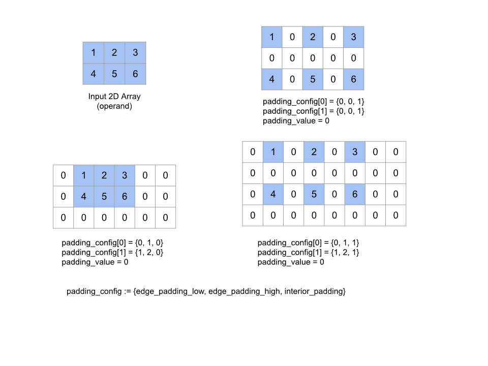
Espande l'array operand specificato inserendo la spaziatura interna intorno all'array e tra gli elementi dell'array con il valore padding_value specificato. padding_config
specifica la quantità di spaziatura interna dei bordi e quella interna per ogni
dimensione.
PaddingConfig è un campo ripetuto di PaddingConfigDimension, che contiene tre campi per ogni dimensione: edge_padding_low, edge_padding_high e interior_padding.
edge_padding_low e edge_padding_high specificano la quantità di spaziatura interna aggiunta rispettivamente alla fascia bassa (accanto all'indice 0) e alla fascia alta (accanto all'indice più alto) di ogni dimensione. La quantità di spaziatura interna dei bordi può essere negativa: il
valore assoluto di spaziatura interna negativa indica il numero di elementi da rimuovere
dalla dimensione specificata.
interior_padding specifica la quantità di spaziatura interna aggiunta tra due elementi qualsiasi in ogni dimensione; non può essere negativa. La spaziatura interna interna avviene logicamente prima della spaziatura interna del bordo quindi, in caso di spaziatura interna negativa, gli elementi vengono rimossi dall'operando con riempimento interno.
Questa operazione è autonoma se le coppie di spaziatura interna del bordo sono tutte (0, 0) e i valori di spaziatura interna interna sono tutti 0. La figura seguente mostra esempi di valori edge_padding e interior_padding diversi per una matrice bidimensionale.
Recv
Vedi anche
XlaBuilder::Recv.
Recv(shape, channel_handle)
| Argomenti | Tipo | Semantica |
|---|---|---|
shape |
Shape |
forma dei dati da ricevere |
channel_handle |
ChannelHandle |
identificatore univoco per ciascuna coppia di invio/ricevuta |
Riceve i dati della forma specificata da un'istruzione Send in un altro
calcolo che condivide lo stesso handle di canale. Restituisce un
XlaOp per i dati ricevuti.
L'API client dell'operazione Recv rappresenta la comunicazione sincrona.
Tuttavia, l'istruzione è scomposta internamente in 2 istruzioni HLO (Recv e RecvDone) per consentire i trasferimenti di dati asincroni. Vedi anche
HloInstruction::CreateRecv e HloInstruction::CreateRecvDone.
Recv(const Shape& shape, int64 channel_id)
Alloca le risorse necessarie per ricevere i dati da un'istruzione Send con lo stesso channel_id. Restituisce un contesto per le risorse allocate, che viene utilizzato da una seguente istruzione RecvDone per attendere il completamento del trasferimento dei dati. Il contesto è una tupla di {receive buffer (shape), request identifier
(U32)} e può essere utilizzato solo da un'istruzione RecvDone.
RecvDone(HloInstruction context)
Dato un contesto creato da un'istruzione Recv, attende il completamento del trasferimento dei dati e restituisce i dati ricevuti.
Ridurre
Vedi anche
XlaBuilder::Reduce.
Applica una funzione di riduzione a uno o più array in parallelo.
Reduce(operands..., init_values..., computation, dimensions)
| Argomenti | Tipo | Semantica |
|---|---|---|
operands |
Sequenza di N XlaOp |
N array di tipo T_0, ..., T_{N-1}. |
init_values |
Sequenza di N XlaOp |
N scalari di tipo T_0, ..., T_{N-1}. |
computation |
XlaComputation |
calcolo di tipo T_0, ..., T_{N-1}, T_0, ..., T_{N-1} -> Collate(T_0, ..., T_{N-1}). |
dimensions |
Array int64 |
di dimensioni non ordinate da ridurre. |
Dove:
- N deve essere maggiore o uguale a 1.
- Il calcolo deve essere associativo "approssimativamente" (vedi sotto).
- Tutte le matrici di input devono avere le stesse dimensioni.
- Tutti i valori iniziali devono formare un'identità in
computation. - Se
N = 1,Collate(T)èT. - Se
N > 1,Collate(T_0, ..., T_{N-1})è una tupla diNelementi di tipoT.
Questa operazione riduce una o più dimensioni di ogni array di input in scalari.
Il rango di ogni array restituito è rank(operand) - len(dimensions). L'output dell'operazione è Collate(Q_0, ..., Q_N), dove Q_i è un array di tipo T_i le cui dimensioni sono descritte di seguito.
Backend diversi possono riassociare il calcolo della riduzione. Ciò può portare a differenze numeriche, poiché alcune funzioni di riduzione come l'aggiunta non sono associative per i numeri in virgola mobile. Tuttavia, se l'intervallo dei dati è limitato, l'aggiunta in virgola mobile è quasi abbastanza associativa per gli utilizzi più pratici.
Esempi
Quando esegui la riduzione in una dimensione in un singolo array 1D con valori [10, 11,
12, 13], con la funzione di riduzione f (questo è computation), il calcolo potrebbe essere eseguito come
f(10, f(11, f(12, f(init_value, 13)))
ma ci sono anche molte altre possibilità, ad es.
f(init_value, f(f(10, f(init_value, 11)), f(f(init_value, 12), f(init_value, 13))))
Di seguito è riportato un esempio approssimativo di pseudocodice di come implementare la riduzione, utilizzando la somma come calcolo della riduzione con un valore iniziale pari a 0.
result_shape <- remove all dims in dimensions from operand_shape

# Iterate over all elements in result_shape. The number of r's here is equal
# to the rank of the result
for r0 in range(result_shape[0]), r1 in range(result_shape[1]), ...:
  # Initialize this result element
  result[r0, r1...] <- 0

  # Iterate over all the reduction dimensions
  for d0 in range(dimensions[0]), d1 in range(dimensions[1]), ...:
    # Increment the result element with the value of the operand's element.
    # The index of the operand's element is constructed from all ri's and di's
    # in the right order (by construction ri's and di's together index over the
    # whole operand shape).
    result[r0, r1...] += operand[ri... di]
Ecco un esempio di riduzione di un array 2D (matrice). La forma ha rango 2, dimensione 0 nella dimensione 2 e dimensione 1 nella dimensione 3:
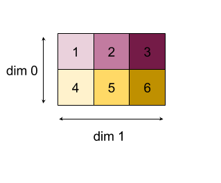
Risultati della riduzione delle dimensioni di 0 o 1 con una funzione "aggiungi":
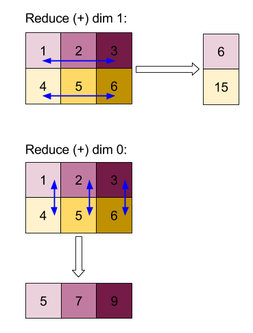
Nota che entrambi i risultati della riduzione sono array 1D. Per comodità visiva, il diagramma mostra una colonna e l'altra come riga.
Per un esempio più complesso, ecco un array 3D. Il suo ranking è 3, dimensione 0 per taglia 4, dimensione 1 per taglia 2 e dimensione 2 per taglia 3. Per semplicità, i valori da 1 a 6 vengono replicati nella dimensione 0.
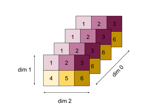
Come nel caso dell'esempio 2D, possiamo ridurre una sola dimensione. Se riduciamo la dimensione 0, ad esempio, otteniamo un array di ranking 2 in cui tutti i valori della dimensione 0 sono stati piegati in uno scalare:
|  4   8  12 |
| 16  20  24 |
Se riduciamo la dimensione 2, otteniamo anche un array di rango-2 in cui tutti i valori della dimensione 2 sono stati piegati in uno scalare:
| 6  15 |
| 6  15 |
| 6  15 |
| 6  15 |
Tieni presente che l'ordine relativo tra le dimensioni rimanenti nell'input viene conservato nell'output, ma ad alcune dimensioni potrebbero essere assegnati nuovi numeri (poiché il ranking cambia).
Possiamo anche ridurre più dimensioni. La riduzione delle dimensioni 0 e 1 produce
l'array 1D [20, 28, 36].
Se riduci l'array 3D su tutte le sue dimensioni, si ottiene lo scalare 84.
Riduzione variadica
Quando N > 1, l'applicazione della funzione "Riduci" è leggermente più complessa, poiché viene applicata
contemporaneamente a tutti gli input. Gli operandi vengono forniti al
calcolo nel seguente ordine:
- Valore ridotto per il primo operando
- ...
- Esecuzione del valore ridotto per l'operando n°
- Valore di input per il primo operando
- ...
- Valore di input per l'operando n'
Ad esempio, considera la seguente funzione di riduzione, che può essere utilizzata per calcolare il valore massimo e l'argmax di un array 1D in parallelo:
f: (Float, Int, Float, Int) -> Float, Int
f(max, argmax, value, index):
  if value >= max:
    return (value, index)
  else:
    return (max, argmax)
Per gli array di input 1-D V = Float[N], K = Int[N] e i valori init I_V = Float, I_K = Int, il risultato f_(N-1) della riduzione sull'unica dimensione di input è equivalente alla seguente applicazione ricorsiva:
f_0 = f(I_V, I_K, V_0, K_0)
f_1 = f(f_0.first, f_0.second, V_1, K_1)
...
f_(N-1) = f(f_(N-2).first, f_(N-2).second, V_(N-1), K_(N-1))
L'applicazione di questa riduzione a un array di valori e a un array di indici sequenziali (iota), co-itererà sugli array e restituirà una tupla contenente il valore massimo e l'indice corrispondente.
ReducePrecision
Vedi anche
XlaBuilder::ReducePrecision.
Modella l'effetto della conversione dei valori in virgola mobile in un formato a precisione inferiore (come IEEE-FP16) e riportandolo al formato originale. Il numero di bit di esponente e mantissa nel formato a precisione inferiore può essere specificato in modo arbitrario, anche se tutte le dimensioni in bit potrebbero non essere supportate su tutte le implementazioni hardware.
ReducePrecision(operand, mantissa_bits, exponent_bits)
| Argomenti | Tipo | Semantica |
|---|---|---|
operand |
XlaOp |
array di tipo con virgola mobile T. |
exponent_bits |
int32 |
numero di bit esponenti nel formato a precisione inferiore |
mantissa_bits |
int32 |
numero di bit mantissa in formato a precisione inferiore |
Il risultato è un array di tipo T. I valori di input vengono arrotondati al valore più vicino rappresentabile con il numero specificato di bit di mantissa (utilizzando la semantica " legami a pari"). Tutti i valori che superano l'intervallo specificato dal numero di bit di esponenti vengono bloccati su un valore infinito positivo o negativo. I valori NaN vengono conservati, anche se possono essere convertiti in valori NaN canonici.
Il formato con precisione inferiore deve avere almeno un bit esponente (per distinguere un valore zero da un infinito, poiché entrambi hanno una mantissa zero) e deve avere un numero non negativo di bit di mantissa. Il numero di bit di esponente o mantissa può superare il valore corrispondente per il tipo T; la porzione corrispondente della conversione è quindi semplicemente no-op.
ReduceScatter
Vedi anche
XlaBuilder::ReduceScatter.
ReduceScatter è un'operazione collettiva che esegue efficacemente un'operazione AllReduce e
poi disperde il risultato suddividendolo in blocchi shard_count lungo
scatter_dimension e la replica i nel gruppo di replica riceve lo shard ith.
ReduceScatter(operand, computation, scatter_dim, shard_count,
replica_group_ids, channel_id)
| Argomenti | Tipo | Semantica |
|---|---|---|
operand |
XlaOp |
Array o una tupla non vuota di array da ridurre nelle repliche. |
computation |
XlaComputation |
Calcolo della riduzione |
scatter_dimension |
int64 |
Dimensione a dispersione. |
shard_count |
int64 |
Numero di blocchi da suddividere scatter_dimension |
replica_groups |
vettore di vettori di int64 |
Gruppi tra i quali vengono eseguite le riduzioni |
channel_id |
int64 facoltativo |
ID canale facoltativo per la comunicazione tra moduli |
- Quando
operandè una tupla di array, la riduzione della dispersione viene eseguita su ciascun elemento della tupla. replica_groupsè un elenco di gruppi di repliche tra cui viene eseguita la riduzione (l'ID replica della replica attuale può essere recuperato utilizzandoReplicaId). L'ordine delle repliche in ogni gruppo determina l'ordine in cui il risultato di AllReduce sarà disperso.replica_groupsdeve essere vuoto (in questo caso tutte le repliche appartengono a un solo gruppo) o contenere lo stesso numero di elementi del numero di repliche. Se è presente più di un gruppo di repliche, tutti devono avere le stesse dimensioni. Ad esempio,replica_groups = {0, 2}, {1, 3}esegue la riduzione tra le repliche0e2,1e3, quindi disperde il risultato.shard_countè la dimensione di ogni gruppo di repliche. È necessario nei casi in cuireplica_groupsè vuoto. Sereplica_groupsnon è vuoto,shard_countdeve essere uguale alle dimensioni di ogni gruppo di repliche.channel_idviene utilizzato per la comunicazione tra moduli: solo le operazionireduce-scattercon lo stessochannel_idpossono comunicare tra loro.
La forma di output è la forma di input con scatter_dimension reso
shard_count volte più piccolo. Ad esempio, se ci sono due repliche e l'operando ha rispettivamente il valore [1.0, 2.25] e [3.0, 5.25] sulle due repliche, il valore di output di questa operazione in cui scatter_dim è 0 sarà [4.0] per la prima replica e [7.5] per la seconda.
ReduceWindow
Vedi anche
XlaBuilder::ReduceWindow.
Applica una funzione di riduzione a tutti gli elementi in ciascuna finestra di una sequenza di N array multidimensionali, producendo come output una singola o tupla di N array multidimensionali. Ogni array di output ha lo stesso numero di elementi del numero di posizioni valide della finestra. Un livello di pooling può essere espresso come ReduceWindow. Analogamente a Reduce, il computation applicato
supera sempre il init_values sul lato sinistro.
ReduceWindow(operands..., init_values..., computation, window_dimensions,
window_strides, padding)
| Argomenti | Tipo | Semantica |
|---|---|---|
operands |
N XlaOps |
Una sequenza di N array multidimensionali di tipo T_0,..., T_{N-1}, ognuno dei quali rappresenta l'area di base su cui è posizionata la finestra. |
init_values |
N XlaOps |
I valori iniziali di N per la riduzione, uno per ciascuno degli operandi N. Vedi Ridurre per i dettagli. |
computation |
XlaComputation |
Funzione di riduzione di tipo T_0, ..., T_{N-1}, T_0, ..., T_{N-1} -> Collate(T_0, ..., T_{N-1}), da applicare agli elementi in ogni finestra di tutti gli operandi di input. |
window_dimensions |
ArraySlice<int64> |
array di numeri interi per i valori delle dimensioni della finestra |
window_strides |
ArraySlice<int64> |
array di numeri interi per i valori dell'andatura finestra |
base_dilations |
ArraySlice<int64> |
array di numeri interi per i valori di dilatazione base |
window_dilations |
ArraySlice<int64> |
array di numeri interi per i valori di dilatazione delle finestre |
padding |
Padding |
tipo di spaziatura interna per la finestra (Padding::kSame, che riempie in modo da avere la stessa forma di output dell'input se il passo è 1 oppure Padding::kValid, che non usa spaziatura interna e "ferma" la finestra quando non è più adatta) |
Dove:
- N deve essere maggiore o uguale a 1.
- Tutte le matrici di input devono avere le stesse dimensioni.
- Se
N = 1,Collate(T)èT. - Se
N > 1,Collate(T_0, ..., T_{N-1})è una tupla diNelementi di tipo(T0,...T{N-1}).
Il codice e la figura riportati di seguito mostrano un esempio di utilizzo di ReduceWindow. L'input è una matrice di dimensioni [4x6] e sia window_dimensions che window_stride_dimensions sono [2x3].
// Create a computation for the reduction (maximum).
XlaComputation max;
{
  XlaBuilder builder(client_, "max");
  auto y = builder.Parameter(0, ShapeUtil::MakeShape(F32, {}), "y");
  auto x = builder.Parameter(1, ShapeUtil::MakeShape(F32, {}), "x");
  builder.Max(y, x);
  max = builder.Build().value();
}

// Create a ReduceWindow computation with the max reduction computation.
XlaBuilder builder(client_, "reduce_window_2x3");
auto shape = ShapeUtil::MakeShape(F32, {4, 6});
auto input = builder.Parameter(0, shape, "input");
builder.ReduceWindow(
    input,
    /*init_val=*/builder.ConstantLiteral(LiteralUtil::MinValue(F32)),
    *max,
    /*window_dimensions=*/{2, 3},
    /*window_stride_dimensions=*/{2, 3},
    Padding::kValid);
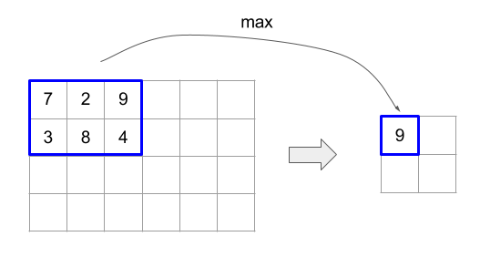
L'intervallo di 1 in una dimensione indica che la posizione di una finestra nella dimensione è di un elemento lontano dalla finestra adiacente. Per specificare che nessuna finestra si sovrappone tra loro, window_stride_dimensions deve essere uguale a window_dimensions. La figura seguente illustra l'uso di due diversi valori di passo. La spaziatura interna viene applicata a ogni dimensione dell'input e i calcoli sono gli stessi, come se l'input venisse fornito con le dimensioni che ha dopo la spaziatura interna.
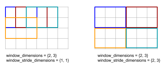
Per un esempio di spaziatura interna non banale, valuta la possibilità di calcolare il minimo della finestra di riduzione
(il valore iniziale è MAX_FLOAT) con la dimensione 3 e di eseguire l'intervallo 2 sull'array di input [10000, 1000, 100, 10, 1]. La spaziatura interna kValid calcola i valori minimi su due finestre
valide: [10000, 1000, 100] e [100, 10, 1], ottenendo
l'output [100, 1]. La spaziatura interna kSame riempie prima l'array in modo che la forma dopo
la riduzione della finestra sia la stessa dell'input per la spaziatura uno, aggiungendo elementi
iniziali su entrambi i lati, ottenendo [MAX_VALUE, 10000, 1000, 100, 10, 1,
MAX_VALUE]. L'esecuzione di reduce-window sull'array riempito opera su tre
finestre [MAX_VALUE, 10000, 1000], [1000, 100, 10], [10, 1, MAX_VALUE] e
rendimento [1000, 10, 1].
L'ordine di valutazione della funzione di riduzione è arbitrario e può essere non deterministico. Pertanto, la funzione di riduzione non deve essere eccessivamente sensibile alla riassociazione. Per ulteriori dettagli, vedi la discussione sull'assocività nel
contesto di Reduce.
ReplicaId
Vedi anche
XlaBuilder::ReplicaId.
Restituisce l'ID univoco (scalare U32) della replica.
ReplicaId()
L'ID univoco di ogni replica è un numero intero senza segno nell'intervallo [0, N), dove N è il numero di repliche. Poiché tutte le repliche eseguono lo stesso
programma, una chiamata ReplicaId() nel programma restituirà un valore diverso su
ogni replica.
Rimodellare
Vedi anche
XlaBuilder::Reshape
e l'operazione Collapse.
Modifica le dimensioni di un array in una nuova configurazione.
Reshape(operand, new_sizes)
Reshape(operand, dimensions, new_sizes)
| Argomenti | Tipo | Semantica |
|---|---|---|
operand |
XlaOp |
array di tipo T |
dimensions |
int64 vettore |
ordine di compressione delle dimensioni |
new_sizes |
int64 vettore |
vettore di dimensioni di nuove dimensioni |
Concettualmente, la funzione "rimodella" appiattisce prima un array in un vettore unidimensionale di valori di dati, quindi perfeziona questo vettore in una nuova forma. Gli argomenti di input sono un array arbitrario di tipo T, un vettore costante di tempo di compilazione degli indici delle dimensioni e un vettore della costante di tempo di compilazione delle dimensioni di dimensione per il risultato.
I valori nel vettore dimension, se fornito, devono essere una permutazione di tutte le dimensioni di T; il valore predefinito se non viene fornito è {0, ..., rank - 1}. L'ordine delle dimensioni in dimensions va dalla dimensione con le variazioni più lente (la più importante) alla dimensione più variabile (la più bassa) nel nidificazione del loop, che comprime l'array di input in un'unica dimensione. Il vettore new_sizes determina la dimensione
dell'array di output. Il valore all'indice 0 in new_sizes è la dimensione della dimensione 0, il valore all'indice 1 è la dimensione della dimensione 1 e così via. Il prodotto delle dimensioni new_size deve essere uguale al prodotto delle dimensioni delle dimensioni dell'operando. Durante il perfezionamento dell'array compresso nell'array multidimensionale definito da new_sizes, le dimensioni in new_sizes sono ordinate a partire da quella con variazione più lenta (maggiore) a quella con variazione più rapida (la più minore).
Ad esempio, supponiamo che v sia un array di 24 elementi:
let v = f32[4x2x3] { { {10, 11, 12}, {15, 16, 17} },
                    { {20, 21, 22}, {25, 26, 27} },
                    { {30, 31, 32}, {35, 36, 37} },
                    { {40, 41, 42}, {45, 46, 47} } };

In-order collapse:
let v012_24 = Reshape(v, {0,1,2}, {24});
then v012_24 == f32[24] {10, 11, 12, 15, 16, 17, 20, 21, 22, 25, 26, 27,
                         30, 31, 32, 35, 36, 37, 40, 41, 42, 45, 46, 47};

let v012_83 = Reshape(v, {0,1,2}, {8,3});
then v012_83 == f32[8x3] { {10, 11, 12}, {15, 16, 17},
                          {20, 21, 22}, {25, 26, 27},
                          {30, 31, 32}, {35, 36, 37},
                          {40, 41, 42}, {45, 46, 47} };

Out-of-order collapse:
let v021_24 = Reshape(v, {1,2,0}, {24});
then v012_24 == f32[24]  {10, 20, 30, 40, 11, 21, 31, 41, 12, 22, 32, 42,
                          15, 25, 35, 45, 16, 26, 36, 46, 17, 27, 37, 47};

let v021_83 = Reshape(v, {1,2,0}, {8,3});
then v021_83 == f32[8x3] { {10, 20, 30}, {40, 11, 21},
                          {31, 41, 12}, {22, 32, 42},
                          {15, 25, 35}, {45, 16, 26},
                          {36, 46, 17}, {27, 37, 47} };


let v021_262 = Reshape(v, {1,2,0}, {2,6,2});
then v021_262 == f32[2x6x2] { { {10, 20}, {30, 40},
                              {11, 21}, {31, 41},
                              {12, 22}, {32, 42} },
                             { {15, 25}, {35, 45},
                              {16, 26}, {36, 46},
                              {17, 27}, {37, 47} } };
Nel caso speciale, con la rimodellazione puoi trasformare un array di un singolo elemento in uno scalare e viceversa. Ad esempio:
Reshape(f32[1x1] { {5} }, {0,1}, {}) == 5;
Reshape(5, {}, {1,1}) == f32[1x1] { {5} };
Inverti (inversione)
Vedi anche
XlaBuilder::Rev.
Rev(operand, dimensions)
| Argomenti | Tipo | Semantica |
|---|---|---|
operand |
XlaOp |
array di tipo T |
dimensions |
ArraySlice<int64> |
dimensioni da invertire |
Inverte l'ordine degli elementi nell'array operand lungo il valore dimensions specificato, generando un array di output della stessa forma. Ogni elemento dell'array di operandi in un indice multidimensionale viene archiviato nell'array di output in un indice trasformato. L'indice multidimensionale viene trasformato invertendo l'indice in ogni dimensione da invertire (ad esempio, se una dimensione di dimensione N è una delle dimensioni invertite, il suo indice i viene trasformato in N - 1 - i).
L'operazione Rev viene utilizzata per invertire l'array di peso della convoluzione lungo le due dimensioni della finestra durante il calcolo del gradiente nelle reti neurali.
RngNormal
Vedi anche
XlaBuilder::RngNormal.
Crea un output di una data forma con numeri casuali generati seguendo la \(N(\mu, \sigma)\) distribuzione normale. I parametri \(\mu\) e \(\sigma\)e la forma di output devono essere di tipo elementare in virgola mobile. I parametri devono inoltre avere un valore scalare.
RngNormal(mu, sigma, shape)
| Argomenti | Tipo | Semantica |
|---|---|---|
mu |
XlaOp |
Scalare di tipo T che specifica la media dei numeri generati |
sigma |
XlaOp |
Scalare di tipo T che specifica la deviazione standard dei |
shape |
Shape |
Forma di output di tipo T |
RngUniform
Vedi anche
XlaBuilder::RngUniform.
Crea un output di una data forma con numeri casuali generati seguendo la distribuzione uniforme nell'intervallo \([a,b)\). I parametri e il tipo di elemento di output devono essere di tipo booleano, integrale o con rappresentazione in virgola mobile, e i tipi devono essere coerenti. I backend di CPU e GPU attualmente supportano solo F64, F32, F16, BF16, S64, U64, S32 e U32. Inoltre, i parametri devono avere un valore scalare. Se \(b <= a\) il risultato è definito dall'implementazione.
RngUniform(a, b, shape)
| Argomenti | Tipo | Semantica |
|---|---|---|
a |
XlaOp |
Scalare di tipo T che specifica il limite inferiore dell'intervallo |
b |
XlaOp |
Scalare di tipo T che specifica il limite superiore dell'intervallo |
shape |
Shape |
Forma di output di tipo T |
RngBitGenerator
Genera un output con una data forma piena di bit casuali uniformi utilizzando l'algoritmo specificato (o il valore predefinito del backend) e restituisce uno stato aggiornato (con la stessa forma dello stato iniziale) e i dati casuali generati.
Lo stato iniziale è lo stato iniziale dell'attuale generazione di numeri casuali. La forma richiesta e i valori validi dipendono dall'algoritmo utilizzato.
È garantito che l'output sia una funzione deterministica dello stato iniziale, ma non è garantito che sia deterministico tra backend e versioni diverse del compilatore.
RngBitGenerator(algorithm, key, shape)
| Argomenti | Tipo | Semantica |
|---|---|---|
algorithm |
RandomAlgorithm |
l'algoritmo PRNG da utilizzare. |
initial_state |
XlaOp |
Stato iniziale dell'algoritmo PRNG. |
shape |
Shape |
Forma di output per i dati generati. |
Valori disponibili per algorithm:
rng_default: algoritmo specifico di backend con requisiti di forma specifici del backend.rng_three_fry: algoritmo PRNG basato su contatore di ThreeFry. La formainitial_stateèu64[2]con valori arbitrari. Salmon et al. SC 2011. Numeri casuali paralleli: facile come 1, 2, 3.rng_philox: algoritmo Philox per generare numeri casuali in parallelo. La formainitial_stateèu64[3]con valori arbitrari. Salmon et al. SC 2011. Numeri casuali paralleli: facile come 1, 2, 3.
A dispersione
L'operazione di dispersione XLA genera una sequenza di risultati che sono i valori dell'array di input operands, con diverse sezioni (in corrispondenza degli indici specificati da scatter_indices) aggiornate con la sequenza di valori in updates utilizzando update_computation.
Vedi anche
XlaBuilder::Scatter.
scatter(operands..., scatter_indices, updates..., update_computation,
index_vector_dim, update_window_dims, inserted_window_dims,
scatter_dims_to_operand_dims)
| Argomenti | Tipo | Semantica |
|---|---|---|
operands |
Sequenza di N XlaOp |
N array dei tipi T_0, ..., T_N in cui distribuire. |
scatter_indices |
XlaOp |
Array contenente gli indici iniziali delle sezioni che devono essere disperse. |
updates |
Sequenza di N XlaOp |
N array di tipo T_0, ..., T_N. updates[i] contiene i valori che devono essere utilizzati per la dispersione di operands[i]. |
update_computation |
XlaComputation |
Calcolo da utilizzare per combinare i valori esistenti nell'array di input e gli aggiornamenti durante la dispersione. Questo calcolo deve essere di tipo T_0, ..., T_N, T_0, ..., T_N -> Collate(T_0, ..., T_N). |
index_vector_dim |
int64 |
La dimensione in scatter_indices che contiene gli indici iniziali. |
update_window_dims |
ArraySlice<int64> |
L'insieme di dimensioni in forma updates che sono dimensioni finestra. |
inserted_window_dims |
ArraySlice<int64> |
L'insieme di dimensioni finestra che deve essere inserita nella forma updates. |
scatter_dims_to_operand_dims |
ArraySlice<int64> |
Una mappa delle dimensioni dagli indici a dispersione allo spazio dell'indice degli operandi. Questo array viene interpretato come mappatura di i a scatter_dims_to_operand_dims[i] . Deve essere one-to-one e totale. |
indices_are_sorted |
bool |
Indica se è garantito che gli indici siano ordinati dal chiamante. |
Dove:
- N deve essere maggiore o uguale a 1.
operands[0], ...,operands[N-1] devono avere tutti le stesse dimensioni.updates[0], ...,updates[N-1] devono avere tutti le stesse dimensioni.- Se
N = 1,Collate(T)èT. - Se
N > 1,Collate(T_0, ..., T_N)è una tupla diNelementi di tipoT.
Se index_vector_dim è uguale a scatter_indices.rank, consideriamo implicitamente scatter_indices come una dimensione 1 finale.
Definiamo update_scatter_dims di tipo ArraySlice<int64> come l'insieme di
dimensioni in forma updates che non sono in update_window_dims, in ordine
crescente.
Gli argomenti della dispersione devono seguire questi vincoli:
Ogni array
updatesdeve avere rangoupdate_window_dims.size + scatter_indices.rank - 1.I limiti della dimensione
iin ogni arrayupdatesdevono essere conformi a quanto segue:- Se
iè presente inupdate_window_dims(ossia uguale aupdate_window_dims[k] perk), il limite della dimensioneiinupdatesnon deve superare il limite corrispondente dioperanddopo aver preso in considerazioneinserted_window_dims(ovveroadjusted_window_bounds[k], doveadjusted_window_boundscontiene i limiti dioperandcon i limiti degli indiciinserted_window_dimsrimossi). - Se
iè presente inupdate_scatter_dims(ovvero è uguale aupdate_scatter_dims[k] perk), il limite della dimensioneiinupdatesdeve essere uguale al limite corrispondente discatter_indices, saltandoindex_vector_dim(ad esempioscatter_indices.shape.dims[k], sek<index_vector_dimescatter_indices.shape.dims[k+1] in caso contrario).
- Se
update_window_dimsdeve essere in ordine crescente, non deve contenere numeri di dimensione ripetuti e deve essere compreso nell'intervallo[0, updates.rank).inserted_window_dimsdeve essere in ordine crescente, non deve contenere numeri di dimensione ripetuti e deve essere compreso nell'intervallo[0, operand.rank).operand.rankdeve essere uguale alla somma diupdate_window_dims.sizeeinserted_window_dims.size.scatter_dims_to_operand_dims.sizedeve essere uguale ascatter_indices.shape.dims[index_vector_dim] e i suoi valori devono essere compresi nell'intervallo[0, operand.rank).
Per un determinato indice U in ogni array updates, l'indice corrispondente I nell'array operands corrispondente in cui deve essere applicato l'aggiornamento viene calcolato come segue:
- Consenti
G= {U[k] perkinupdate_scatter_dims}. UsaGper cercare un vettore di indiceSnell'arrayscatter_indicesin modo tale cheS[i] =scatter_indices[Combina(G,i)] dove Combina(A, b) inserisce b nelle posizioniindex_vector_dimin A. - Crea un indice
SininoperandutilizzandoSdisperdendoSutilizzando la mappascatter_dims_to_operand_dims. In modo più formale:Sin[scatter_dims_to_operand_dims[k]] =S[k] sek<scatter_dims_to_operand_dims.size.Sin[_] =0altrimenti.
- Crea un indice
Winin ogni arrayoperandsdisperdendo gli indici aupdate_window_dimsinUsecondoinserted_window_dims. In modo più formale:Win[window_dims_to_operand_dims(k)] =U[k] seksi trova inupdate_window_dims, dovewindow_dims_to_operand_dimsè la funzione monotonica con dominio [0,update_window_dims.size) e intervallo [0,operand.rank) \inserted_window_dims. Ad esempio, seupdate_window_dims.sizeè4,operand.rankè6einserted_window_dimsè {0,2} allorawindow_dims_to_operand_dimsè {0→1,1→3,2→4,3→5}.Win[_] =0altrimenti.
IèWin+Sin, dove + è l'aggiunta a livello di elemento.
In sintesi, l'operazione di dispersione può essere definita come segue.
- Inizializza
outputconoperands, ovvero per tutti gli indiciJ, per tutti gli indiciOnell'arrayoperands[J]:
output[J][O] =operands[J][O] - Per ogni indice
Unell'arrayupdates[J] e l'indice corrispondenteOnell'arrayoperand[J], seOè un indice valido peroutput:
(output[0][O], ...,output[N-1][O]) =update_computation(output[0][O], ..., ,output[N-1][O],updates[0][U], ...,updates[N-1][U])
L'ordine in cui vengono applicati gli aggiornamenti non è deterministico. Di conseguenza, quando più indici in updates fanno riferimento allo stesso indice in operands, il valore corrispondente in output sarà non deterministico.
Tieni presente che il primo parametro trasmesso in update_computation sarà sempre il valore corrente dell'array output, mentre il secondo sarà sempre il valore dell'array updates. Questo è importante
in particolare per i casi in cui il valore update_computation non è commutativo.
Se indices_are_sorted è impostato su true, XLA può presupporre che le start_indices
vengano ordinate (in ordine crescente (start_index_map)) dall'utente. In caso contrario,
la semantica è l'implementazione definita.
In modo informale, l'operazione a dispersione può essere vista come un'inversa dell'operazione di raccolta, ovvero l'operazione di dispersione aggiorna gli elementi nell'input estratti dall'operazione di raccolta corrispondente.
Per una descrizione informale dettagliata ed esempi, consulta la sezione "Descrizione informale" in Gather.
Seleziona
Vedi anche
XlaBuilder::Select.
Crea un array di output dagli elementi di due matrici di input, in base ai valori di un array di predicato.
Select(pred, on_true, on_false)
| Argomenti | Tipo | Semantica |
|---|---|---|
pred |
XlaOp |
array di tipo PRED |
on_true |
XlaOp |
array di tipo T |
on_false |
XlaOp |
array di tipo T |
Gli array on_true e on_false devono avere la stessa forma. È anche la forma
dell'array di output. L'array pred deve avere la stessa dimensionalità di
on_true e on_false, con il tipo di elemento PRED.
Per ogni elemento P di pred, l'elemento corrispondente dell'array di output
viene recuperato da on_true se il valore di P è true e da on_false se il
valore di P è false. Come forma limitata di trasmissione,
pred può essere un tipo scalare di tipo PRED. In questo caso, l'array di output viene preso interamente da on_true se pred è true e da on_false se pred è false.
Esempio con pred non scalabile:
let pred: PRED[4] = {true, false, false, true};
let v1: s32[4] = {1, 2, 3, 4};
let v2: s32[4] = {100, 200, 300, 400};
==>
Select(pred, v1, v2) = s32[4]{1, 200, 300, 4};
Esempio con pred scalare:
let pred: PRED = true;
let v1: s32[4] = {1, 2, 3, 4};
let v2: s32[4] = {100, 200, 300, 400};
==>
Select(pred, v1, v2) = s32[4]{1, 2, 3, 4};
Le selezioni tra le tuple sono supportate. Per questo scopo le tuple sono considerate
tipi scalari. Se on_true e on_false sono tuple (che devono avere la stessa forma!), pred deve essere uno scalare di tipo PRED.
SelectAndScatter
Vedi anche
XlaBuilder::SelectAndScatter.
Questa operazione può essere considerata come un'operazione composita che prima calcola
ReduceWindow sull'array operand per selezionare un elemento da ogni finestra, poi disperde l'array source negli indici degli elementi selezionati per
costruire un array di output con la stessa forma dell'array di operandi. La funzione select binaria viene utilizzata per selezionare un elemento da ogni finestra applicandolo a ogni finestra e viene chiamata con la proprietà secondo cui il vettore di indice del primo parametro è lessicograficamente inferiore al vettore di indice del secondo parametro. La funzione select restituisce true se il primo parametro è selezionato e false se il secondo parametro è selezionato e la funzione deve mantenere transitività (ad esempio, se select(a, b) e select(b, c) sono true, anche select(a, c) è true), in modo che l'elemento selezionato non dipenda dall'ordine degli elementi attraversati per una determinata finestra.
La funzione scatter viene applicata a ciascun indice selezionato nell'array di output. Prevede due parametri scalari:
- Valore corrente nell'indice selezionato nell'array di output
- Il valore di dispersione di
sourceche si applica all'indice selezionato
Combina i due parametri e restituisce un valore scalare utilizzato per aggiornare il valore nell'indice selezionato nell'array di output. Inizialmente, tutti gli indici dell'array di output sono impostati su init_value.
L'array di output ha la stessa forma dell'array operand, mentre l'array source deve avere la stessa forma del risultato dell'applicazione di un'operazione ReduceWindow sull'array operand. SelectAndScatter può essere usato per retropropagare i valori del gradiente per un livello di pooling in una rete neurale.
SelectAndScatter(operand, select, window_dimensions, window_strides,
padding, source, init_value, scatter)
| Argomenti | Tipo | Semantica |
|---|---|---|
operand |
XlaOp |
array di tipo T su cui scorrono le finestre |
select |
XlaComputation |
calcolo binario di tipo T, T -> PRED, da applicare a tutti gli elementi in ogni finestra; restituisce true se è selezionato il primo parametro e false se è selezionato il secondo parametro |
window_dimensions |
ArraySlice<int64> |
array di numeri interi per i valori delle dimensioni della finestra |
window_strides |
ArraySlice<int64> |
array di numeri interi per i valori dell'andatura finestra |
padding |
Padding |
tipo di spaziatura interna per la finestra (Padding::kSame o Padding::kValid) |
source |
XlaOp |
array di tipo T con i valori a dispersione |
init_value |
XlaOp |
valore scalare di tipo T per il valore iniziale dell'array di output |
scatter |
XlaComputation |
calcolo binario di tipo T, T -> T, per applicare ogni elemento di origine a dispersione con il relativo elemento di destinazione |
La figura seguente mostra esempi di utilizzo di SelectAndScatter, in cui la funzione select
che calcola il valore massimo tra i suoi parametri. Tieni presente che quando le finestre si sovrappongono, come nella figura (2) di seguito, un indice dell'array operand può essere selezionato più volte da finestre diverse. Nella figura, l'elemento con valore 9 viene selezionato da entrambe le finestre principali (blu e rosso), mentre la funzione di aggiunta binaria scatter produce l'elemento di output con valore 8 (2 + 6).
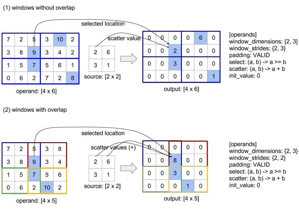
L'ordine di valutazione della funzione scatter è arbitrario e può essere
non deterministico. Di conseguenza, la funzione scatter non deve essere eccessivamente sensibile alla riassociazione. Per ulteriori dettagli, vedi la discussione sull'assocività nel
contesto di Reduce.
Invia
Vedi anche
XlaBuilder::Send.
Send(operand, channel_handle)
| Argomenti | Tipo | Semantica |
|---|---|---|
operand |
XlaOp |
dati da inviare (array di tipo T) |
channel_handle |
ChannelHandle |
identificatore univoco per ciascuna coppia di invio/ricevuta |
Invia i dati dell'operando specificati a un'istruzione Recv in un altro calcolo che condivide lo stesso handle del canale. Non restituisce alcun dato.
Analogamente all'operazione Recv, l'API client dell'operazione Send rappresenta la comunicazione sincrona ed è scomposta internamente in due istruzioni HLO (Send e SendDone) per consentire i trasferimenti di dati asincroni. Vedi anche
HloInstruction::CreateSend e HloInstruction::CreateSendDone.
Send(HloInstruction operand, int64 channel_id)
Avvia un trasferimento asincrono dell'operando alle risorse allocate dall'istruzione Recv con lo stesso ID canale. Restituisce un contesto, che viene utilizzato da una seguente istruzione SendDone per attendere il completamento del trasferimento di dati. Il contesto è una tupla di {operando (forma), ID richiesta (U32)} e può essere utilizzato solo da un'istruzione SendDone.
SendDone(HloInstruction context)
Dato un contesto creato da un'istruzione Send, attende il completamento del trasferimento dei dati. L'istruzione non restituisce alcun dato.
Programmazione delle istruzioni del canale
L'ordine di esecuzione delle 4 istruzioni per ciascun canale (Recv, RecvDone,
Send, SendDone) è il seguente.
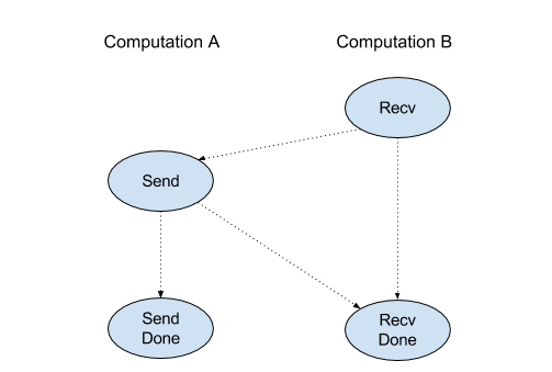
Recvavviene prima delSendSendavviene prima delRecvDoneRecvavviene prima delRecvDoneSendavviene prima delSendDone
Quando i compilatori backend generano una pianificazione lineare per ogni calcolo che comunica tramite istruzioni di canale, non devono esserci cicli tra i calcoli. Ad esempio, le pianificazioni riportate di seguito portano a deadlock.
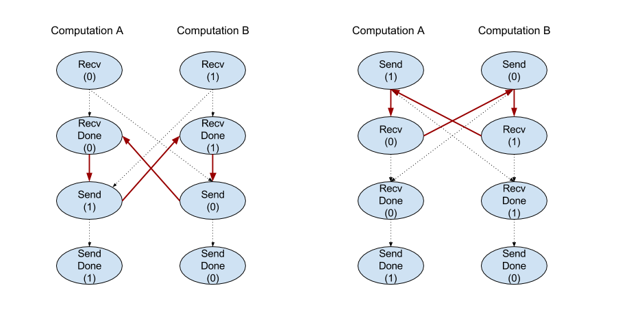
Sezione
Vedi anche
XlaBuilder::Slice.
La suddivisione estrae un sottoarray dall'array di input. Il sottoarray ha lo stesso ranking dell'input e contiene i valori all'interno di un riquadro di delimitazione all'interno dell'array di input in cui le dimensioni e gli indici del riquadro di delimitazione vengono forniti come argomenti per l'operazione sezione.
Slice(operand, start_indices, limit_indices, strides)
| Argomenti | Tipo | Semantica |
|---|---|---|
operand |
XlaOp |
Matrice dimensionale N di tipo T |
start_indices |
ArraySlice<int64> |
Elenco di N numeri interi contenenti gli indici iniziali della sezione per ogni dimensione. I valori devono essere maggiori o uguali a zero. |
limit_indices |
ArraySlice<int64> |
Elenco di N numeri interi contenenti gli indici finali (esclusivi) per la sezione di ogni dimensione. Ciascun valore deve essere maggiore o uguale al rispettivo valore start_indices per la dimensione e minore o uguale alla dimensione della dimensione. |
strides |
ArraySlice<int64> |
Elenco di N numeri interi che decide l'intervallo di input della sezione. La sezione seleziona ogni elemento strides[d] nella dimensione d. |
Esempio unidimensionale:
let a = {0.0, 1.0, 2.0, 3.0, 4.0}
Slice(a, {2}, {4}) produces:
  {2.0, 3.0}
Esempio bidimensionale:
let b =
 { {0.0,  1.0,  2.0},
   {3.0,  4.0,  5.0},
   {6.0,  7.0,  8.0},
   {9.0, 10.0, 11.0} }

Slice(b, {2, 1}, {4, 3}) produces:
  { { 7.0,  8.0},
    {10.0, 11.0} }
Ordina
Vedi anche
XlaBuilder::Sort.
Sort(operands, comparator, dimension, is_stable)
| Argomenti | Tipo | Semantica |
|---|---|---|
operands |
ArraySlice<XlaOp> |
Gli operandi da ordinare. |
comparator |
XlaComputation |
Il calcolo di confronto da utilizzare. |
dimension |
int64 |
La dimensione in base alla quale ordinare. |
is_stable |
bool |
Indica se utilizzare un ordinamento stabile. |
Se viene fornito un solo operando:
Se l'operando è un tensore di rango-1 (una matrice), il risultato è una matrice ordinata. Se vuoi ordinare l'array in ordine crescente, il comparatore deve eseguire un confronto di tipo "minore di". Formalmente, dopo l'ordinamento, l'array rimane valido per tutte le posizioni dell'indice
i, jconi < jche può esserecomparator(value[i], value[j]) = comparator(value[j], value[i]) = falseocomparator(value[i], value[j]) = true.Se l'operando ha un ranking più elevato, l'operando viene ordinato in base alla dimensione fornita. Ad esempio, per un tensore di ranking 2 (una matrice), un valore di dimensione
0ordina in modo indipendente ogni colonna, mentre un valore della dimensione1ordina ogni riga in modo indipendente. Se non viene fornito alcun numero di dimensione, per impostazione predefinita viene scelta l'ultima dimensione. Per la dimensione ordinata, viene applicato lo stesso ordine utilizzato nel caso in cui il ranking è 1.
Se vengono forniti gli operandi n > 1:
Tutti gli operandi
ndevono essere tensori con le stesse dimensioni. I tipi di elementi dei tensori possono essere diversi.Tutti gli operandi sono ordinati insieme, non individualmente. Concettualmente, gli operandi vengono trattati come tupla. Quando controlli se gli elementi di ogni operando nelle posizioni di indice
iejdevono essere scambiati, il comparatore viene chiamato con i parametri scalari2 * n, dove il parametro2 * kcorrisponde al valore nella posizioneidell'operandok-the il parametro2 * k + 1corrisponde al valore nella posizionejdell'operandok-th. In genere, il comparatore confronta i parametri2 * ke2 * k + 1tra loro e potrebbe utilizzare altre coppie di parametri come elementi di fermatura.Il risultato è una tupla composta dagli operandi in ordine (lungo la dimensione fornita, come sopra). L'operando
i-thdella tupla corrisponde all'operandoi-thdi Ordina.
Ad esempio, se sono presenti tre operandi operand0 = [3, 1],
operand1 = [42, 50], operand2 = [-3.0, 1.1] e il comparatore confronta solo i valori di operand0 con minore di, l'output di questo ordinamento è la tupla ([1, 3], [50, 42], [1.1, -3.0]).
Se is_stable è impostato su true, viene garantito che l'ordinamento sia stabile, ovvero, se ci sono elementi considerati uguali dal comparatore, l'ordine relativo dei valori uguali viene mantenuto. Due elementi e1 e e2 sono
uguali se e solo se comparator(e1, e2) = comparator(e2, e1) = false. Per impostazione predefinita, is_stable è impostato su false.
Transpose
Vedi anche l'operazione tf.reshape.
Transpose(operand)
| Argomenti | Tipo | Semantica |
|---|---|---|
operand |
XlaOp |
L'operando da trasporre. |
permutation |
ArraySlice<int64> |
Come modificare le dimensioni. |
Rimuove le dimensioni dell'operando con la permutazione specificata, quindi
∀ i . 0 ≤ i < rank ⇒ input_dimensions[permutation[i]] = output_dimensions[i].
È uguale a Reshape(operando, permutazione, Permute(permutazione, operando.forma.dimensioni)).
TriangularSolve
Vedi anche
XlaBuilder::TriangularSolve.
Risolve sistemi di equazioni lineari con matrici a coefficiente triangolare inferiore o superiore per sostituzione in avanti o indietro. Trasmettendo lungo le dimensioni principali, questa routine risolve uno dei sistemi matriciali op(a) * x =
b, o x * op(a) = b, per la variabile x, dati a e b, dove op(a) è op(a) = a, op(a) = Transpose(a) o op(a) = Conj(Transpose(a)).
TriangularSolve(a, b, left_side, lower, unit_diagonal, transpose_a)
| Argomenti | Tipo | Semantica |
|---|---|---|
a |
XlaOp |
un array con rango > 2 di tipo complesso o con virgola mobile con forma [..., M, M]. |
b |
XlaOp |
un array di ranking > 2 dello stesso tipo con forma [..., M, K] se left_side è true, [..., K, M] in caso contrario. |
left_side |
bool |
indica se risolvere un sistema nel formato op(a) * x = b (true) o x * op(a) = b (false). |
lower |
bool |
se utilizzare il triangolo superiore o inferiore di a. |
unit_diagonal |
bool |
se true, si presume che gli elementi diagonali di a siano 1 e non siano accessibili. |
transpose_a |
Transpose |
se utilizzare a così com'è, trasporlo o prenderne la trasposizione coniugata. |
I dati di input vengono letti solo dal triangolo inferiore/superiore di a, a seconda del
valore di lower. I valori dell'altro triangolo vengono ignorati. I dati di output vengono restituiti nello stesso triangolo; i valori nell'altro triangolo sono definiti dall'implementazione e possono essere qualsiasi cosa.
Se il ranking di a e b è maggiore di 2, vengono trattati come batch di
matrici, dove tutte le dimensioni tranne le 2 secondarie sono dimensioni batch. a e
b devono avere dimensioni batch uguali.
Tupla
Vedi anche
XlaBuilder::Tuple.
Una tupla contenente un numero variabile di handle di dati, ognuno dei quali ha una propria forma.
È un'operazione analoga a quella di std::tuple in C++. Concettualmente:
let v: f32[10] = f32[10]{0, 1, 2, 3, 4, 5, 6, 7, 8, 9};
let s: s32 = 5;
let t: (f32[10], s32) = tuple(v, s);
È possibile scomporre le tuple (accessibile) tramite l'operazione GetTupleElement.
La funzione
Vedi anche
XlaBuilder::While.
While(condition, body, init)
| Argomenti | Tipo | Semantica |
|---|---|---|
condition |
XlaComputation |
XlaComputation di tipo T -> PRED, che definisce la condizione di terminazione del loop. |
body |
XlaComputation |
XlaComputation di tipo T -> T, che definisce il corpo del loop. |
init |
T |
Valore iniziale per il parametro di condition e body. |
Esegue in sequenza body fino a quando condition non funziona. Questo è simile a un tipico loop "and" in molte altre lingue, ad eccezione delle differenze e delle restrizioni elencate di seguito.
- Un nodo
Whilerestituisce un valore di tipoT, che è il risultato dell'ultima esecuzione delbody. - La forma del tipo
Tviene determinata in modo statico e deve essere la stessa in tutte le iterazioni.
I parametri T dei calcoli vengono inizializzati con il valore init nella prima iterazione e vengono aggiornati automaticamente in base al nuovo risultato di body in ogni iterazione successiva.
Un caso d'uso principale del nodo While è implementare l'esecuzione ripetuta dell'addestramento nelle reti neurali. Lo pseudocodice semplificato è mostrato di seguito con un grafico che rappresenta il calcolo. Il codice è disponibile in
while_test.cc.
Il tipo T in questo esempio è un Tuple composto da int32 per il conteggio delle iterazioni e vector[10] per l'accumulatore. Per 1000 iterazioni, il loop continua ad aggiungere un vettore costante all'accumulatore.
// Pseudocode for the computation.
init = {0, zero_vector[10]} // Tuple of int32 and float[10].
result = init;
while (result(0) < 1000) {
  iteration = result(0) + 1;
  new_vector = result(1) + constant_vector[10];
  result = {iteration, new_vector};
}