다음은 XlaBuilder 인터페이스에 정의된 작업의 시맨틱을 설명합니다. 일반적으로 이러한 작업은 xla_data.proto의 RPC 인터페이스에 정의된 작업에 일대일로 매핑됩니다.
명명법 참고 사항: XLA에서 처리하는 일반화된 데이터 유형은 일정한 유형 (예: 32비트 부동)의 요소를 포함하는 N차원 배열입니다. 이 문서에서 배열은 임의의 차원 배열을 나타내는 데 사용됩니다. 편의를 위해 특수 사례에는 더 구체적이고 익숙한 이름이 사용됩니다. 예를 들어 벡터는 1차원 배열이고 행렬은 2차원 배열입니다.
AfterAll
XlaBuilder::AfterAll도 참고하세요.
AfterAll은 다양한 개수의 토큰을 취하여 단일 토큰을 생성합니다. 토큰은 부작용 작업 사이에 스레드되어 순서를 적용할 수 있는 기본 유형입니다. AfterAll는 집합 작업 후에 작업을 정렬하기 위한 토큰의 조인으로 사용할 수 있습니다.
AfterAll(operands)
| 인수 | 유형 | 시맨틱 |
|---|---|---|
operands |
XlaOp |
가변 토큰 수 |
AllGather
XlaBuilder::AllGather도 참고하세요.
복제본 간에 연결을 수행합니다.
AllGather(operand, all_gather_dim, shard_count, replica_group_ids,
channel_id)
| 인수 | 유형 | 시맨틱 |
|---|---|---|
operand
|
XlaOp
|
복제본 간에 연결할 배열 |
all_gather_dim |
int64 |
연결 측정기준 |
replica_groups
|
int64 벡터로 구성된
벡터 |
연결이 수행되는 그룹 사이에 |
channel_id
|
선택사항 int64
|
교차 모듈 통신을 위한 채널 ID(선택사항) |
replica_groups는 연결이 수행되는 복제본 그룹 목록입니다 (ReplicaId를 사용하여 현재 복제본의 복제본 ID를 가져올 수 있음). 각 그룹의 복제본 순서에 따라 입력이 결과에 포함되는 순서가 결정됩니다.replica_groups은 비어 있거나 (0부터N - 1까지 정렬된 단일 그룹에 속함) 복제본 수와 동일한 수의 요소를 포함해야 합니다. 예를 들어replica_groups = {0, 2}, {1, 3}은 복제본0및2, 그리고1와3간에 연결을 수행합니다.shard_count는 각 복제본 그룹의 크기입니다.replica_groups가 비어 있는 경우에 필요합니다.channel_id는 모듈 간 통신에 사용됩니다. 동일한channel_id가 있는all-gather작업만 서로 통신할 수 있습니다.
출력 셰이프는 all_gather_dim가 shard_count배 더 커진 입력 셰이프입니다. 예를 들어 복제본이 2개 있고 피연산자의 복제본 2개에서 각각 [1.0, 2.5]와 [3.0, 5.25] 값이 있으면 all_gather_dim가 0인 이 작업의 출력 값은 두 복제본에서 [1.0, 2.5, 3.0,
5.25]가 됩니다.
AllReduce
XlaBuilder::AllReduce도 참고하세요.
복제본 간에 커스텀 계산을 수행합니다.
AllReduce(operand, computation, replica_group_ids, channel_id)
| 인수 | 유형 | 시맨틱 |
|---|---|---|
operand
|
XlaOp
|
여러 복제본의 크기를 줄일 배열의 배열 또는 비어 있지 않은 튜플입니다. |
computation |
XlaComputation |
감소 계산 |
replica_groups
|
int64 벡터로 구성된
벡터 |
감축이 수행되는 그룹들 사이에 |
channel_id
|
선택사항 int64
|
교차 모듈 통신을 위한 채널 ID(선택사항) |
operand가 배열의 튜플이면 튜플의 각 요소에 대해 모두 축소가 실행됩니다.replica_groups는 축소가 수행되는 복제본 그룹 목록입니다 (ReplicaId를 사용하여 현재 복제본의 복제본 ID를 가져올 수 있음).replica_groups는 비어 있거나 (이 경우 모든 복제본이 단일 그룹에 속) 복제본 수와 동일한 수의 요소를 포함해야 합니다. 예를 들어replica_groups = {0, 2}, {1, 3}는 복제본0와2,1와3간에 축소를 수행합니다.channel_id는 모듈 간 통신에 사용됩니다. 동일한channel_id가 있는all-reduce작업만 서로 통신할 수 있습니다.
출력 모양은 입력 모양과 동일합니다. 예를 들어 복제본이 2개 있고 피연산자의 복제본 2개에서 각각 [1.0, 2.5]와 [3.0, 5.25] 값이 있는 경우, 두 복제본의 이 작업 및 합계 계산의 출력 값은 [4.0, 7.75]가 됩니다. 입력이 튜플이면 출력도 튜플입니다.
AllReduce의 결과를 계산하려면 각 복제본의 입력이 하나씩 있어야 합니다. 따라서 한 복제본이 다른 복제본보다 AllReduce 노드를 여러 번 실행하면 이전 복제본은 영원히 대기합니다. 복제본이 모두 같은 프로그램을 실행하므로 이러한 상황이 발생할 수 있는 방법은 많지 않지만 while 루프의 조건이 인피드의 데이터에 종속되는 경우와 삽입된 데이터로 인해 while 루프가 다른 복제본보다 여러 번 반복하게 되는 경우 가능합니다.
AllToAll
XlaBuilder::AllToAll도 참고하세요.
AllToAll은 모든 코어에서 모든 코어로 데이터를 전송하는 집합적인 작업입니다. 다음 두 단계로 구성됩니다.
- 분산형 단계. 각 코어에서 피연산자는
split_dimensions를 따라split_count개수의 블록으로 분할되며, 블록은 모든 코어에 분산됩니다. 예를 들어 i번째 블록은 i번째 코어로 전송됩니다. - 수집 단계. 각 코어는 수신된 블록을
concat_dimension를 따라 연결합니다.
참여 코어는 다음과 같이 구성할 수 있습니다.
replica_groups: 각 ReplicaGroup에는 계산에 참여하는 복제본 ID 목록이 포함됩니다 (현재 복제본의 복제본 ID는ReplicaId를 사용하여 가져올 수 있음). AllToAll은 하위 그룹 내에서 지정된 순서대로 적용됩니다. 예를 들어replica_groups = { {1,2,3}, {4,5,0} }는 AllToAll이 복제본{1, 2, 3}내에서 수집 단계에서 적용되며 수신된 블록은 1, 2, 3의 동일한 순서로 연결된다는 의미입니다. 그런 다음 복제본 4, 5, 0 내에 또 다른 AllToAll이 적용되며 연결 순서도 4, 5, 0입니다.replica_groups가 비어 있으면 모든 복제본은 표시된 순서대로 하나의 그룹에 속합니다.
기본 요건:
split_dimension에 있는 피연산자의 차원 크기는split_count로 나눌 수 있습니다.- 피연산자의 형태가 튜플이 아닙니다.
AllToAll(operand, split_dimension, concat_dimension, split_count,
replica_groups)
| 인수 | 유형 | 시맨틱 |
|---|---|---|
operand |
XlaOp |
N차원 입력 배열 |
split_dimension
|
int64
|
피연산자가 분할되는 측정기준의 이름을 지정하는 [0,
n) 간격의 값 |
concat_dimension
|
int64
|
분할 블록이 연결되는 측정기준의 이름을 지정하는 [0,
n) 간격의 값 |
split_count
|
int64
|
이 작업에 참여하는 코어 수입니다. replica_groups가 비어 있으면 이 값은 복제본 수여야 합니다. 그렇지 않으면 각 그룹의 복제본 수와 같아야 합니다. |
replica_groups
|
ReplicaGroup 벡터
|
각 그룹에는 복제본 ID 목록이 포함됩니다. |
다음은 Alltoall의 예입니다.
XlaBuilder b("alltoall");
auto x = Parameter(&b, 0, ShapeUtil::MakeShape(F32, {4, 16}), "x");
AllToAll(x, /*split_dimension=*/1, /*concat_dimension=*/0, /*split_count=*/4);
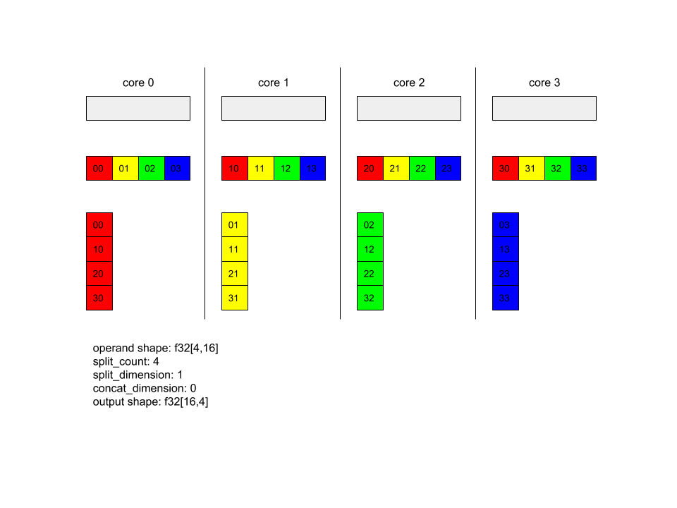
이 예시에서는 Alltoall에 참여하는 4개의 코어가 있습니다. 각 코어에서 피연산자는 측정기준 0을 따라 4개의 부분으로 분할되므로 각 부분의 형태는 f32[4,4]입니다. 4개 부분은 모든 코어에 분산됩니다. 그런 다음 각 코어는 수신된 부분을 코어 0~4의 순서대로 차원 1에 따라 연결합니다. 따라서 각 코어의 출력은 f32[16,4] 형태를 취합니다.
BatchNormGrad
알고리즘에 대한 자세한 설명은 XlaBuilder::BatchNormGrad 및 배치 정규화 문서 원본을 참조하세요.
배치 norm의 경사를 계산합니다.
BatchNormGrad(operand, scale, mean, variance, grad_output, epsilon, feature_index)
| 인수 | 유형 | 시맨틱 |
|---|---|---|
operand |
XlaOp |
정규화할 n차원 배열 (x) |
scale |
XlaOp |
1차원 배열 (\(\gamma\)) |
mean |
XlaOp |
1차원 배열 (\(\mu\)) |
variance |
XlaOp |
1차원 배열 (\(\sigma^2\)) |
grad_output |
XlaOp |
BatchNormTraining에 전달된 그라데이션 (\(\nabla y\)) |
epsilon |
float |
입실론 값 (\(\epsilon\)) |
feature_index |
int64 |
operand의 지형지물 측정기준 색인 |
특성 차원의 각 특성 (feature_index는 operand의 특성 차원에 대한 색인)의 경우 연산은 다른 모든 차원에 걸쳐 operand, offset, scale를 기준으로 경사를 계산합니다. feature_index는
operand의 특성 차원에 대한 유효한 색인이어야 합니다.
3개의 경사는 다음 공식으로 정의됩니다 (4차원 배열을 operand, 특징 차원 지수 l, 배치 크기 m, 공간 크기 w, h로 가정).
\[ \begin{split} c_l&= \frac{1}{mwh}\sum_{i=1}^m\sum_{j=1}^w\sum_{k=1}^h \left( \nabla y_{ijkl} \frac{x_{ijkl} - \mu_l}{\sigma^2_l+\epsilon} \right) \\\\ d_l&= \frac{1}{mwh}\sum_{i=1}^m\sum_{j=1}^w\sum_{k=1}^h \nabla y_{ijkl} \\\\ \nabla x_{ijkl} &= \frac{\gamma_{l} }{\sqrt{\sigma^2_{l}+\epsilon} } \left( \nabla y_{ijkl} - d_l - c_l (x_{ijkl} - \mu_{l}) \right) \\\\ \nabla \gamma_l &= \sum_{i=1}^m\sum_{j=1}^w\sum_{k=1}^h \left( \nabla y_{ijkl} \frac{x_{ijkl} - \mu_l}{\sqrt{\sigma^2_{l}+\epsilon} } \right) \\\\\ \nabla \beta_l &= \sum_{i=1}^m\sum_{j=1}^w\sum_{k=1}^h \nabla y_{ijkl} \end{split} \]
입력 mean와 variance는 배치 및 공간 차원의 모멘트 값을 나타냅니다.
출력 유형은 핸들 3개로 구성된 튜플입니다.
| 출력 | 유형 | 시맨틱 |
|---|---|---|
grad_operand
|
XlaOp
|
입력 operand에 대한 기울기 ($\nabla
x$) |
grad_scale
|
XlaOp
|
입력 scale에 대한 기울기 ($\nabla
\gamma$) |
grad_offset
|
XlaOp
|
입력 offset에 대한 기울기($\nabla
\beta$) |
BatchNormInference
알고리즘에 대한 자세한 설명은 XlaBuilder::BatchNormInference 및 배치 정규화 문서 원본을 참조하세요.
배치 및 공간 차원에 걸쳐 배열을 정규화합니다.
BatchNormInference(operand, scale, offset, mean, variance, epsilon, feature_index)
| 인수 | 유형 | 시맨틱 |
|---|---|---|
operand |
XlaOp |
정규화할 N차원 배열 |
scale |
XlaOp |
1차원 배열 |
offset |
XlaOp |
1차원 배열 |
mean |
XlaOp |
1차원 배열 |
variance |
XlaOp |
1차원 배열 |
epsilon |
float |
입실론 값 |
feature_index |
int64 |
operand의 지형지물 측정기준 색인 |
특성 차원의 각 특성 (feature_index는 operand에 있는 특성 차원의 색인)에 대해 연산은 다른 모든 차원의 평균과 분산을 계산하고 평균과 분산을 사용하여 operand의 각 요소를 정규화합니다. feature_index는 operand의 지형지물 차원에 대한 유효한 색인이어야 합니다.
BatchNormInference은 각 배치에 대해 mean 및 variance를 계산하지 않고 BatchNormTraining를 호출하는 것과 같습니다. 대신 입력 mean 및 variance를 추정값으로 사용합니다. 이 작업의 목적은 추론의 지연 시간을 줄이는 것으로, 이름은 BatchNormInference입니다.
출력은 입력 operand와 형태가 동일한 정규화된 N차원 배열입니다.
BatchNormTraining
알고리즘에 관한 자세한 설명은 XlaBuilder::BatchNormTraining 및 the original batch normalization paper도 참고하세요.
배치 및 공간 차원에 걸쳐 배열을 정규화합니다.
BatchNormTraining(operand, scale, offset, epsilon, feature_index)
| 인수 | 유형 | 시맨틱 |
|---|---|---|
operand |
XlaOp |
정규화할 n차원 배열 (x) |
scale |
XlaOp |
1차원 배열 (\(\gamma\)) |
offset |
XlaOp |
1차원 배열 (\(\beta\)) |
epsilon |
float |
입실론 값 (\(\epsilon\)) |
feature_index |
int64 |
operand의 지형지물 측정기준 색인 |
특성 차원의 각 특성 (feature_index는 operand에 있는 특성 차원의 색인)에 대해 연산은 다른 모든 차원의 평균과 분산을 계산하고 평균과 분산을 사용하여 operand의 각 요소를 정규화합니다. feature_index는 operand의 지형지물 차원에 대한 유효한 색인이어야 합니다.
공간 차원의 크기가 w 및 h인 m 요소를 포함하는 operand \(x\) 의 각 배치에 대해 알고리즘이 다음과 같이 적용됩니다 (operand가 4차원 배열이라고 가정).
특성 차원의 각 특성에 대한 \(\mu_l\) 배치 평균을
l계산합니다. \(\mu_l=\frac{1}{mwh}\sum_{i=1}^m\sum_{j=1}^w\sum_{k=1}^h x_{ijkl}\)배치 분산 계산 \(\sigma^2_l\): $\sigma^2l=\frac{1}{mwh}\sum{i=1}^m\sum{j=1}^w\sum{k=1}^h (x_{ijkl} - \mu_l)^2$
정규화, 확장, 이동:\(y_{ijkl}=\frac{\gamma_l(x_{ijkl}-\mu_l)}{\sqrt[2]{\sigma^2_l+\epsilon} }+\beta_l\)
0으로 나누기 오류를 방지하기 위해 일반적으로 작은 숫자인 epsilon 값이 추가됩니다.
출력 유형은 XlaOp 세 개의 튜플입니다.
| 출력 | 유형 | 시맨틱 |
|---|---|---|
output
|
XlaOp
|
입력 operand (y)와 모양이 동일한 n차원 배열 |
batch_mean |
XlaOp |
1차원 배열 (\(\mu\)) |
batch_var |
XlaOp |
1차원 배열 (\(\sigma^2\)) |
batch_mean 및 batch_var는 위의 수식을 사용하여 배치 및 공간 차원에서 계산된 순간입니다.
BitcastConvertType
XlaBuilder::BitcastConvertType도 참고하세요.
TensorFlow의 tf.bitcast와 마찬가지로 데이터 도형에서 타겟 도형으로 요소별 비트캐스트 작업을 실행합니다. 입력 및 출력 크기는 일치해야 합니다. 예를 들어 s32 요소는 비트캐스트 루틴을 통해 f32 요소가 되고 s32 요소는 4개의 s8 요소가 됩니다. Bitcast는 하위 수준의 변환으로 구현되므로 부동 소수점 표현이 다른 머신은 다른 결과를 제공합니다.
BitcastConvertType(operand, new_element_type)
| 인수 | 유형 | 시맨틱 |
|---|---|---|
operand |
XlaOp |
희미한 D가 있는 유형 T의 배열 |
new_element_type |
PrimitiveType |
U 유형 |
마지막 측정기준은 변환 전후의 원시 크기의 비율에 따라 변하는 것을 제외하고 피연산자와 타겟 도형의 측정기준이 일치해야 합니다.
소스 및 대상 요소 유형은 튜플이 아니어야 합니다.
다른 너비의 원시 유형으로 비트캐스트 변환
BitcastConvert HLO 명령은 출력 요소 유형 T'의 크기가 입력 요소 T의 크기와 같지 않은 경우를 지원합니다. 전체 작업은 개념적으로 비트캐스트이고 기본 바이트를 변경하지 않으므로 출력 요소의 모양이 변경되어야 합니다. B = sizeof(T), B' =
sizeof(T')에는 두 가지 경우가 있을 수 있습니다.
먼저 B > B'인 경우 출력 셰이프는 가장 작은 차원의 새로운 크기인 B/B'를 가져옵니다. 예를 들면 다음과 같습니다.
f16[10,2]{1,0} %output = f16[10,2]{1,0} bitcast-convert(f32[10]{0} %input)
효과적인 스칼라의 경우 규칙은 동일하게 유지됩니다.
f16[2]{0} %output = f16[2]{0} bitcast-convert(f32[] %input)
또는 B' > B의 경우 명령어에 입력 형태의 마지막 논리 차원이 B'/B와 같아야 하며 이 차원은 변환 중에 삭제됩니다.
f32[10]{0} %output = f32[10]{0} bitcast-convert(f16[10,2]{1,0} %input)
서로 다른 비트 너비 간의 변환은 요소별로 적용되지 않습니다.
방송
XlaBuilder::Broadcast도 참고하세요.
배열의 데이터를 복제하여 배열에 차원을 추가합니다.
Broadcast(operand, broadcast_sizes)
| 인수 | 유형 | 시맨틱 |
|---|---|---|
operand |
XlaOp |
복제할 배열입니다. |
broadcast_sizes |
ArraySlice<int64> |
새 크기의 크기 |
새 차원은 왼쪽에 삽입됩니다. 즉, broadcast_sizes에 값이 {a0, ..., aN}이고 피연산자 도형의 차원이 {b0, ..., bM}이면 출력의 도형은 차원 {a0, ..., aN, b0, ..., bM}이 됩니다.
새 측정기준은 피연산자의 사본(예:
output[i0, ..., iN, j0, ..., jM] = operand[j0, ..., jM]
예를 들어 operand가 값이 2.0f인 스칼라 f32이고 broadcast_sizes가 {2, 3}이면 결과는 f32[2, 3] 형태가 있는 배열이 되고 결과의 모든 값은 2.0f가 됩니다.
BroadcastInDim
XlaBuilder::BroadcastInDim도 참고하세요.
배열의 데이터를 복제하여 배열의 크기와 순위를 확장합니다.
BroadcastInDim(operand, out_dim_size, broadcast_dimensions)
| 인수 | 유형 | 시맨틱 |
|---|---|---|
operand |
XlaOp |
복제할 배열입니다. |
out_dim_size |
ArraySlice<int64> |
대상 도형의 크기 |
broadcast_dimensions |
ArraySlice<int64> |
타겟 도형에서 피연산자 도형의 각 차원이 어디에 해당하는 차원인가 |
브로드캐스트와 비슷하지만 어디서나 크기를 추가하고 크기 1로 기존 크기를 확장할 수 있습니다.
operand는 out_dim_size에 설명된 도형으로 브로드캐스트됩니다.
broadcast_dimensions는 operand의 크기를 타겟 도형의 크기에 매핑합니다. 즉, 피연산자의 i번째 차원은 출력 도형의 broadcast_dimension[i]번째 차원에 매핑됩니다. operand의 차원은 크기가 1이거나 매핑되는 출력 형태의 치수와 같아야 합니다. 나머지 크기는 크기 1로 채워집니다. 그런 다음 이 퇴적 차원을 따라 브로드캐스트하여 출력 셰이프에 도달합니다. 시맨틱은 브로드캐스트 페이지에 자세히 설명되어 있습니다.
통화
XlaBuilder::Call도 참고하세요.
지정된 인수로 계산을 호출합니다.
Call(computation, args...)
| 인수 | 유형 | 시맨틱 |
|---|---|---|
computation |
XlaComputation |
임의 유형의 N 매개변수를 사용하는 T_0, T_1, ..., T_{N-1} -> S 유형 계산 |
args |
N개의 XlaOp 시퀀스 |
임의 유형의 N 인수 |
args의 인수 및 유형은 computation의 매개변수와 일치해야 합니다. args가 없어야 합니다.
콜레스키
XlaBuilder::Cholesky도 참고하세요.
대칭 (에르미트안) 양의 정적 행렬 배치의 콜레스키 분해를 계산합니다.
Cholesky(a, lower)
| 인수 | 유형 | 시맨틱 |
|---|---|---|
a |
XlaOp |
복합 또는 부동 소수점 유형의 순위 > 2 배열. |
lower |
bool |
a의 위쪽 또는 아래쪽 삼각형을 사용할지 여부입니다. |
lower이 true이면 $a = l이 되도록 삼각 행렬 l을 계산합니다 .
l^T$. lower가 false이면\(a = u^T . u\)와 같은 삼각 행렬 u을 계산합니다.
입력 데이터는 lower 값에 따라 a의 아래쪽/위쪽 삼각형에서만 읽힙니다. 다른 삼각형의 값은 무시됩니다. 출력 데이터는 동일한 삼각형에 반환됩니다. 다른 삼각형의 값은 구현이 정의되어 있을 수 있습니다.
a의 순위가 2보다 크면 a는 행렬 배치로 처리되며, 보조 2차원을 제외한 모든 차원은 배치 차원입니다.
a가 대칭 (헤르미타인) 양의 정적이 아닌 경우 결과가 구현으로 정의됩니다.
클램프
XlaBuilder::Clamp도 참고하세요.
최소값과 최대값 사이의 범위 내에 피연산자를 고정합니다.
Clamp(min, operand, max)
| 인수 | 유형 | 시맨틱 |
|---|---|---|
min |
XlaOp |
유형 T의 배열 |
operand |
XlaOp |
유형 T의 배열 |
max |
XlaOp |
유형 T의 배열 |
특정 피연산자와 최솟값 및 최댓값이 주어졌을 때, 피연산자가 최솟값과 최댓값 사이의 범위 내에 있으면 피연산자를 반환하고 그렇지 않으면 피연산자가 이 범위 아래에 있으면 최솟값을 반환하고 피연산자가 이 범위 위에 있으면 최댓값을 반환합니다. 즉, clamp(a, x, b) = min(max(a, x), b)입니다.
세 개의 배열은 모두 동일한 형태여야 합니다. 또는 제한된 형태의 브로드캐스트로서 min 및/또는 max는 T 유형의 스칼라일 수 있습니다.
스칼라 min 및 max 사용 예시:
let operand: s32[3] = {-1, 5, 9};
let min: s32 = 0;
let max: s32 = 6;
==>
Clamp(min, operand, max) = s32[3]{0, 5, 6};
접기
XlaBuilder::Collapse 및 tf.reshape 작업도 참고하세요.
배열의 측정기준을 하나의 측정기준으로 축소합니다.
Collapse(operand, dimensions)
| 인수 | 유형 | 시맨틱 |
|---|---|---|
operand |
XlaOp |
유형 T의 배열 |
dimensions |
int64 벡터 |
T 차원의 연속된 하위집합입니다. |
접기는 피연산자 측정기준의 지정된 하위 집합을 단일 측정기준으로 바꿉니다. 입력 인수는 T 유형의 임의 배열과 차원 색인의 컴파일 시간 상수 벡터입니다. 차원 색인은 T 차원의 연속적인 하위 집합인 순서 (낮은 차원에서 높은 차원의 숫자)여야 합니다. 따라서 {0, 1, 2}, {0, 1} 또는 {1, 2}는 모두 유효한 측정기준 집합이지만 {1, 0} 또는 {0, 2}는 그렇지 않습니다. 이러한 크기는 기존 크기 시퀀스에서 대체된 것과 동일한 위치에 있는 새로운 1개의 새로운 크기로 교체되며, 새 크기 크기는 원래 크기 크기의 곱과 같습니다. dimensions의 최저 차원 숫자는 이러한 차원을 축소하는 루프 중첩에서 가장 느린 변동 차원 (가장 주요한 차원)이며 가장 높은 차원 숫자는 가장 빠르게 변합니다 (가장 작은 차원). 더 일반적인 축소 순서가 필요한 경우 tf.reshape 연산자를 참고하세요.
예를 들어 v를 24개 요소의 배열이라고 가정해 보겠습니다.
let v = f32[4x2x3] { { {10, 11, 12},  {15, 16, 17} },
{ {20, 21, 22},  {25, 26, 27} },
{ {30, 31, 32},  {35, 36, 37} },
{ {40, 41, 42},  {45, 46, 47} } };

// Collapse to a single dimension, leaving one dimension.
let v012 = Collapse(v, {0,1,2});
then v012 == f32[24] {10, 11, 12, 15, 16, 17,
20, 21, 22, 25, 26, 27,
30, 31, 32, 35, 36, 37,
40, 41, 42, 45, 46, 47};

// Collapse the two lower dimensions, leaving two dimensions.
let v01 = Collapse(v, {0,1});
then v01 == f32[4x6] { {10, 11, 12, 15, 16, 17},
{20, 21, 22, 25, 26, 27},
{30, 31, 32, 35, 36, 37},
{40, 41, 42, 45, 46, 47} };

// Collapse the two higher dimensions, leaving two dimensions.
let v12 = Collapse(v, {1,2});
then v12 == f32[8x3] { {10, 11, 12},
{15, 16, 17},
{20, 21, 22},
{25, 26, 27},
{30, 31, 32},
{35, 36, 37},
{40, 41, 42},
{45, 46, 47} };
CollectivePermute
XlaBuilder::CollectivePermute도 참고하세요.
CollectivePermute는 여러 복제본을 보내고 받는 집합적인 작업입니다.
CollectivePermute(operand, source_target_pairs)
| 인수 | 유형 | 시맨틱 |
|---|---|---|
operand |
XlaOp |
N차원 입력 배열 |
source_target_pairs |
<int64, int64> 벡터 |
(source_Replica_id, target_Replica_id) 쌍의 목록입니다. 각 쌍의 경우 피연산자가 소스 복제본에서 대상 복제본으로 전송됩니다. |
source_target_pair에는 다음과 같은 제한사항이 있습니다.
- 두 쌍의 대상 복제본 ID가 같아서는 안 되며 소스 복제본 ID가 같아서는 안 됩니다.
- 복제본 ID가 어떤 쌍의 타겟도 아닌 경우 해당 복제본의 출력은 입력과 형태가 같은 0으로 구성된 텐서입니다.
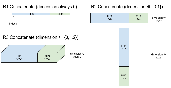
Concatenate
XlaBuilder::ConcatInDim도 참고하세요.
Concatenate는 여러 배열 피연산자로부터 배열을 구성합니다. 배열은 각 입력 배열 피연산자와 순위가 동일하며 (서로 순위가 같아야 함) 지정된 순서대로 인수를 포함합니다.
Concatenate(operands..., dimension)
| 인수 | 유형 | 시맨틱 |
|---|---|---|
operands |
N XlaOp의 시퀀스 |
차원이 [L0, L1, ...]인 T 유형의 N 배열. N >= 1이 필요합니다. |
dimension |
int64 |
operands 간에 연결할 측정기준의 이름을 지정하는 [0, N) 간격의 값입니다. |
dimension를 제외하고 모든 측정기준이 동일해야 합니다. XLA가 '비정형' 배열을 지원하지 않기 때문입니다. 또한 rank-0 값은 연결할 수 없습니다. 연결이 발생하는 차원의 이름을 지정할 수 없기 때문입니다.
1차원 예:
Concat({ {2, 3}, {4, 5}, {6, 7} }, 0)
>>> {2, 3, 4, 5, 6, 7}
2차원 예:
let a = {
{1, 2},
{3, 4},
{5, 6},
};
let b = {
{7, 8},
};
Concat({a, b}, 0)
>>> {
{1, 2},
{3, 4},
{5, 6},
{7, 8},
}
다이어그램:
조건부
XlaBuilder::Conditional도 참고하세요.
Conditional(pred, true_operand, true_computation, false_operand,
false_computation)
| 인수 | 유형 | 시맨틱 |
|---|---|---|
pred |
XlaOp |
PRED 유형의 스칼라 |
true_operand |
XlaOp |
\(T_0\)유형의 인수 |
true_computation |
XlaComputation |
\(T_0 \to S\)유형의 XlaComput |
false_operand |
XlaOp |
\(T_1\)유형의 인수 |
false_computation |
XlaComputation |
\(T_1 \to S\)유형의 XlaComput |
pred가 true이면 true_computation를 실행하고, pred가 false이면 false_computation를 실행하고 결과를 반환합니다.
true_computation는 \(T_0\) 유형의 단일 인수를 사용해야 하며 동일한 유형이어야 하는 true_operand로 호출됩니다. false_computation는 \(T_1\) 유형의 단일 인수를 사용해야 하며 동일한 유형이어야 하는 false_operand로 호출됩니다. true_computation 및 false_computation의 반환된 값의 유형은 동일해야 합니다.
pred 값에 따라 true_computation와 false_computation 중 하나만 실행됩니다.
Conditional(branch_index, branch_computations, branch_operands)
| 인수 | 유형 | 시맨틱 |
|---|---|---|
branch_index |
XlaOp |
S32 유형의 스칼라 |
branch_computations |
N XlaComputation의 시퀀스 |
\(T_0 \to S , T_1 \to S , ..., T_{N-1} \to S\)유형의 XlaComputations |
branch_operands |
N XlaOp의 시퀀스 |
\(T_0 , T_1 , ..., T_{N-1}\)유형의 인수 |
branch_computations[branch_index]를 실행하고 결과를 반환합니다. branch_index가 0보다 작거나 N보다 크거나 같은 S32이면 branch_computations[N-1]가 기본 브랜치로 실행됩니다.
각 branch_computations[b]은 \(T_b\) 유형의 단일 인수를 사용해야 하며 동일한 유형이어야 하는 branch_operands[b]로 호출됩니다. 각 branch_computations[b]의 반환된 값 유형은 동일해야 합니다.
branch_index 값에 따라 branch_computations 중 하나만 실행됩니다.
전환수 (컨볼루션)
XlaBuilder::Conv도 참고하세요.
ConvWithGeneralPadding이 나오지만, 패딩은 SAME 또는 VALID로 간단히 지정됩니다. 동일한 패딩이 스트라이딩을 고려하지 않을 때 입력과 동일한 형태를 갖도록 입력 (lhs)을 0으로 패딩합니다. VALID 패딩은 단순히 패딩이 없음을 의미합니다.
ConvWithGeneralPadding (컨볼루션)
XlaBuilder::ConvWithGeneralPadding도 참고하세요.
신경망에 사용되는 종류의 컨볼루션을 계산합니다. 여기서 컨볼루션은 n차원 기본 영역을 따라 이동하는 N차원 창으로 생각할 수 있으며 윈도우의 가능한 각 위치에 대해 계산이 실행됩니다.
| 인수 | 유형 | 시맨틱 |
|---|---|---|
lhs |
XlaOp |
n+2 입력 배열 순위 지정 |
rhs |
XlaOp |
rank n+2 커널 가중치 배열 |
window_strides |
ArraySlice<int64> |
커널 스트라이드의 n-d 배열 |
padding |
ArraySlice< pair<int64,int64>> |
(낮음, 높은) 패딩의 n-d 배열 |
lhs_dilation |
ArraySlice<int64> |
n-d lhs 팽창 계수 배열 |
rhs_dilation |
ArraySlice<int64> |
n-d Rhs 확장 계수 배열 |
feature_group_count |
int64 | 특성 그룹의 수 |
batch_group_count |
int64 | 배치 그룹 수 |
n은 공간 차원의 개수입니다. lhs 인수는 기본 영역을 설명하는 순위 n+2 배열입니다. 물론 rhs도 입력이지만 이를 입력이라고 합니다. 신경망에서는 이것이 입력 활성화입니다.
n+2 측정기준은 다음 순서로 분류됩니다.
batch: 이 차원의 각 좌표는 컨볼루션이 실행되는 독립 입력을 나타냅니다.z/depth/features: 기본 영역의 각 (y,x) 위치에는 이 차원으로 이동하는 벡터가 연결되어 있습니다.spatial_dims: 창이 이동하는 기본 영역을 정의하는n공간 크기를 설명합니다.
rhs 인수는 컨볼루셔널 필터/커널/창을 설명하는 순위 n+2 배열입니다. 측정기준은 다음 순서로 표시됩니다.
output-z: 출력의z차원입니다.input-z: 이 치수 곱하기feature_group_count의 크기는z단위 크기(lhs)와 같아야 합니다.spatial_dims: 기본 영역을 가로지르는 n-d 윈도우를 정의하는n공간 치수를 설명합니다.
window_strides 인수는 공간 차원에서 컨볼루셔널 구간의 스트라이드를 지정합니다. 예를 들어 첫 번째 공간 차원의 스트라이드가 3이면 창은 첫 번째 공간 색인이 3으로 나눌 수 있는 좌표에만 배치될 수 있습니다.
padding 인수는 베이스 영역에 적용할 0 패딩의 양을 지정합니다. 패딩의 양은 음수일 수 있습니다. 음수 패딩의 절댓값은 컨볼루션을 실행하기 전에 지정된 차원에서 삭제할 요소의 수를 나타냅니다. padding[0]는 차원 y의 패딩을 지정하고 padding[1]는 차원 x의 패딩을 지정합니다. 각 쌍은 첫 번째 요소로 낮은 패딩을, 두 번째 요소로 높은 패딩을 가집니다. 낮은 패딩은 낮은 색인의 방향으로 적용되고 높은 패딩은 높은 색인의 방향으로 적용됩니다. 예를 들어 padding[1]가 (2,3)이면 왼쪽에 2개의 0이 있고 두 번째 공간 차원에 오른쪽에 3개의 0이 있는 패딩이 있습니다. 패딩을 사용하는 것은 컨볼루션을 실행하기 전에 동일한 0 값을 입력 (lhs)에 삽입하는 것과 같습니다.
lhs_dilation 및 rhs_dilation 인수는 각 공간 차원에서 lhs와 rhs에 각각 적용할 확장 계수를 지정합니다. 공간 차원의 확장 계수가 d이면 d-1 구멍이 암시적으로 해당 차원의 각 항목 사이에 배치되어 배열의 크기가 증가합니다. 구멍은 노옵스(no-ops) 값으로 채워집니다. 즉, 컨볼루션의 경우 0을 의미합니다.
RHS의 팽창을 위압 컨볼루션이라고도 합니다. 자세한 내용은 tf.nn.atrous_conv2d를 참고하세요. lhs의 팽창을 전치 컨볼루션이라고도
합니다. 자세한 내용은 tf.nn.conv2d_transpose를 참고하세요.
feature_group_count 인수 (기본값 1)는 그룹화된 컨볼루션에 사용할 수 있습니다. feature_group_count는 입력 특성 차원과 출력 특성 차원 모두의 제수여야 합니다. feature_group_count가 1보다 크면 개념적으로 입력 및 출력 특성 차원과 rhs 출력 특성 차원이 여러 feature_group_count 그룹으로 균일하게 분할되며 각 그룹은 연속적인 하위 시퀀스로 구성됩니다. rhs의 입력 특성 차원은 lhs 입력 특성 차원을 feature_group_count로 나눈 값과 같아야 합니다 (따라서 이미 입력 특성 그룹의 크기가 있어야 함). i번째 그룹은 여러 개의 개별 컨볼루션에 대해 feature_group_count를 계산하는 데 함께 사용됩니다. 이러한 컨볼루션의 결과는 출력 특성 차원에서 함께 연결됩니다.
깊이별 컨볼루션의 경우 feature_group_count 인수는 입력 특성 차원으로 설정되고 필터의 형태는 [filter_height, filter_width, in_channels, channel_multiplier]에서 [filter_height, filter_width, 1, in_channels * channel_multiplier]로 변경됩니다. 자세한 내용은 tf.nn.depthwise_conv2d를 참고하세요.
batch_group_count (기본값 1) 인수는 역전파 중에 그룹화된 필터에 사용할 수 있습니다. batch_group_count는 lhs (입력) 배치 측정기준 크기의 제수여야 합니다. batch_group_count이 1보다 크면 출력 배치 차원의 크기가 input batch
/ batch_group_count여야 한다는 의미입니다. batch_group_count는 출력 특성 크기의 제수여야 합니다.
출력 도형의 차원은 다음과 같은 순서로 지정됩니다.
batch: 이 치수에batch_group_count를 곱한 값은batch치수의 크기(lhs)와 같아야 합니다.z: 커널의output-z와 크기 (rhs)가 동일합니다.spatial_dims: 컨볼루셔널 기간의 각 유효한 배치에 해당하는 하나의 값

위의 그림은 batch_group_count 필드의 작동 방식을 보여줍니다. 실제로 각 lhs 배치를 batch_group_count 그룹으로 분할하고 출력 특성에도 동일한 작업을 수행합니다. 그런 다음 이러한 그룹마다 쌍방향 컨볼루션을
수행하고 출력 특성 차원에 따라 출력을 연결합니다. 다른 모든 차원 (특징 및 공간)의 운영 시맨틱스는 동일하게 유지됩니다.
컨볼루셔널 기간의 유효한 위치는 스트라이드와 패딩 후 기본 영역의 크기에 따라 결정됩니다.
컨볼루션의 기능을 설명하려면 2차원 컨볼루션이 있다고 가정하고 출력에서 고정된 batch, z, y, x 좌표를 선택합니다. 여기서 (y,x)는 기본 영역 내 창의 모서리 위치입니다 (예: 공간 크기를 해석하는 방법에 따라 왼쪽 상단). 이제 각 2차원 점이 1차원 벡터에 연결된 기본 영역에서 가져온 2차원 창이 있으므로 3차원 상자를 얻습니다. 컨볼루셔널 커널에서 출력 좌표 z를 고정했으므로 3D 상자도 있습니다. 두 상자의 치수가 동일하므로 두 상자 간 요소별 곱의 합을 구할 수 있습니다 (내적과 유사). 이것이 출력 값입니다.
예를 들어 output-z가 5이면 창의 각 위치가 출력의 z 차원으로 된 출력의 값 5개를 생성합니다. 이러한 값은 사용되는 컨볼루셔널 커널의 부분이 다릅니다. 각 output-z 좌표에 사용되는 별도의 3차원 값 상자가 있습니다. 따라서 각각 서로 다른 필터를 사용하는 5개의 개별 컨볼루션으로 생각할 수 있습니다.
다음은 패딩과 스트라이딩이 있는 2차원 컨볼루션의 의사 코드입니다.
for (b, oz, oy, ox) {  // output coordinates
  value = 0;
  for (iz, ky, kx) {  // kernel coordinates and input z
    iy = oy*stride_y + ky - pad_low_y;
    ix = ox*stride_x + kx - pad_low_x;
    if ((iy, ix) inside the base area considered without padding) {
      value += input(b, iz, iy, ix) * kernel(oz, iz, ky, kx);
    }
  }
  output(b, oz, oy, ox) = value;
}
ConvertElementType
XlaBuilder::ConvertElementType도 참고하세요.
C++의 요소별 static_cast와 마찬가지로 데이터 도형에서 타겟 도형으로의 요소별 변환 작업을 실행합니다. 크기는 일치해야 하며, 요소별로 변환이 이루어집니다. 예를 들어 s32 요소는 s32에서 f32로의 변환 루틴을 통해 f32 요소가 됩니다.
ConvertElementType(operand, new_element_type)
| 인수 | 유형 | 시맨틱 |
|---|---|---|
operand |
XlaOp |
희미한 D가 있는 유형 T의 배열 |
new_element_type |
PrimitiveType |
U 유형 |
피연산자의 차원과 타겟 셰이프의 차원이 일치해야 합니다. 소스 및 대상 요소 유형은 튜플이 아니어야 합니다.
T=s32에서 U=f32로의 변환과 같은 변환은 가장 가까운 짝수로 반올림과 같은 정규화 int-부동 소수점 변환 루틴을 실행합니다.
let a: s32[3] = {0, 1, 2};
let b: f32[3] = convert(a, f32);
then b == f32[3]{0.0, 1.0, 2.0}
CrossReplicaSum
합계 계산을 사용하여 AllReduce을 수행합니다.
CustomCall
XlaBuilder::CustomCall도 참고하세요.
계산 내에서 사용자 제공 함수를 호출합니다.
CustomCall(target_name, args..., shape)
| 인수 | 유형 | 시맨틱 |
|---|---|---|
target_name |
string |
함수의 이름입니다. 이 기호 이름을 타겟팅하는 호출 명령어가 내보내집니다. |
args |
N개의 XlaOp 시퀀스 |
임의 유형의 N 인수로, 함수에 전달됩니다. |
shape |
Shape |
함수의 출력 셰이프 |
함수 서명은 인수 또는 인수의 유형에 관계없이 동일합니다.
extern "C" void target_name(void* out, void** in);
예를 들어 CustomCall이 다음과 같이 사용된 경우입니다.
let x = f32[2] {1,2};
let y = f32[2x3] { {10, 20, 30}, {40, 50, 60} };

CustomCall("myfunc", {x, y}, f32[3x3])
다음은 myfunc 구현의 예입니다.
extern "C" void myfunc(void* out, void** in) {
  float (&x)[2] = *static_cast<float(*)[2]>(in[0]);
  float (&y)[2][3] = *static_cast<float(*)[2][3]>(in[1]);
  EXPECT_EQ(1, x[0]);
  EXPECT_EQ(2, x[1]);
  EXPECT_EQ(10, y[0][0]);
  EXPECT_EQ(20, y[0][1]);
  EXPECT_EQ(30, y[0][2]);
  EXPECT_EQ(40, y[1][0]);
  EXPECT_EQ(50, y[1][1]);
  EXPECT_EQ(60, y[1][2]);
  float (&z)[3][3] = *static_cast<float(*)[3][3]>(out);
  z[0][0] = x[1] + y[1][0];
  // ...
}
사용자 제공 함수에는 부작용이 없어야 하며 실행은 멱등적이어야 합니다.
Dot
XlaBuilder::Dot도 참고하세요.
Dot(lhs, rhs)
| 인수 | 유형 | 시맨틱 |
|---|---|---|
lhs |
XlaOp |
유형 T의 배열 |
rhs |
XlaOp |
유형 T의 배열 |
이 연산의 정확한 의미 체계는 피연산자의 순위에 따라 다릅니다.
| 입력 | 출력 | 시맨틱 |
|---|---|---|
벡터 [n] dot 벡터 [n] |
스칼라 | 벡터 내적 |
행렬 [m x k] dot 벡터 [k] |
벡터 [m] | 행렬 벡터 곱셈 |
행렬 [m x k] dot 행렬 [k x n] |
행렬 [m x n] | 행렬-행렬 곱셈 |
이 연산은 lhs의 두 번째 측정기준 (또는 순위가 1인 경우 첫 번째 측정기준)과 rhs의 첫 번째 측정기준에 대해 곱의 합계를 수행합니다. 이는 '축약된' 측정기준입니다. lhs와 rhs의 축약된 크기는 크기가 같아야 합니다. 실제로는 벡터, 벡터/행렬 곱셈 또는 행렬/행렬 곱셈 사이의 내적을 구하는 데 사용할 수 있습니다.
DotGeneral
XlaBuilder::DotGeneral도 참고하세요.
DotGeneral(lhs, rhs, dimension_numbers)
| 인수 | 유형 | 시맨틱 |
|---|---|---|
lhs |
XlaOp |
유형 T의 배열 |
rhs |
XlaOp |
유형 T의 배열 |
dimension_numbers |
DotDimensionNumbers |
계약 및 배치 차원 번호 |
Dot과 비슷하지만 lhs과 rhs 모두에 계약 치수 및 배치 치수 번호를 지정할 수 있습니다.
| DotDimensionNumbers 필드 | 유형 | 시맨틱 |
|---|---|---|
lhs_contracting_dimensions
|
반복된 int64 | lhs개의 축소된 측정기준 번호 |
rhs_contracting_dimensions
|
반복된 int64 | rhs개의 축소된 측정기준 번호 |
lhs_batch_dimensions
|
반복된 int64 | 배치 측정기준 번호 lhs개 |
rhs_batch_dimensions
|
반복된 int64 | 배치 측정기준 번호 rhs개 |
DotGeneral은 dimension_numbers에 지정된 계약 크기를 기준으로 제품의 합계를 계산합니다.
lhs 및 rhs의 연결된 계약 치수 번호는 동일하지 않아도 되지만 치수 크기는 동일해야 합니다.
축소된 측정기준 번호의 예:
lhs = { {1.0, 2.0, 3.0},
{4.0, 5.0, 6.0} }

rhs = { {1.0, 1.0, 1.0},
{2.0, 2.0, 2.0} }

DotDimensionNumbers dnums;
dnums.add_lhs_contracting_dimensions(1);
dnums.add_rhs_contracting_dimensions(1);

DotGeneral(lhs, rhs, dnums) -> { {6.0, 12.0},
{15.0, 30.0} }
lhs 및 rhs의 연결된 배치 차원 번호는 치수 크기가 같아야 합니다.
배치 차원 숫자 (배치 크기 2, 2x2 행렬)를 사용한 예:
lhs = { { {1.0, 2.0},
{3.0, 4.0} },
{ {5.0, 6.0},
{7.0, 8.0} } }

rhs = { { {1.0, 0.0},
{0.0, 1.0} },
{ {1.0, 0.0},
{0.0, 1.0} } }

DotDimensionNumbers dnums;
dnums.add_lhs_contracting_dimensions(2);
dnums.add_rhs_contracting_dimensions(1);
dnums.add_lhs_batch_dimensions(0);
dnums.add_rhs_batch_dimensions(0);

DotGeneral(lhs, rhs, dnums) -> { { {1.0, 2.0},
{3.0, 4.0} },
{ {5.0, 6.0},
{7.0, 8.0} } }
| 입력 | 출력 | 시맨틱 |
|---|---|---|
[b0, m, k] dot [b0, k, n] |
[b0, m, n] | 일괄 Matmul |
[b0, b1, m, k] dot [b0, b1, k, n] |
[b0, b1, m, n] | 일괄 Matmul |
결과 차원 번호가 배치 차원으로 시작하여 lhs 비계약/비배치 차원, 마지막으로 rhs 비계약/비배치 차원으로 이어집니다.
DynamicSlice
XlaBuilder::DynamicSlice도 참고하세요.
DynamicSlice는 동적 start_indices의 입력 배열에서 하위 배열을 추출합니다. 각 측정기준의 슬라이스 크기는 각 측정기준에서 배타적 슬라이스 간격의 끝점을 지정하는 size_indices로 전달됩니다(예: [start, start + size). start_indices의 도형은 순위 == 1이고 크기 크기는 operand의 순위와 같아야 합니다.
DynamicSlice(operand, start_indices, size_indices)
| 인수 | 유형 | 시맨틱 |
|---|---|---|
operand |
XlaOp |
유형 T의 N차원 배열 |
start_indices |
N XlaOp의 시퀀스 |
각 차원에 대한 슬라이스의 시작 색인을 포함하는 N개의 스칼라 정수 목록입니다. 값은 0 이상이어야 합니다. |
size_indices |
ArraySlice<int64> |
각 차원의 슬라이스 크기를 포함하는 N개의 정수 목록입니다. 각 값은 0보다 커야 하며, 모듈로 크기 크기를 래핑하지 않도록 시작 + 크기는 측정기준의 크기보다 작거나 같아야 합니다. |
유효한 슬라이스 색인은 슬라이스를 실행하기 전에 [1, N)의 각 색인 i에 다음 변환을 적용하여 계산됩니다.
start_indices[i] = clamp(start_indices[i], 0, operand.dimension_size[i] - size_indices[i])
이렇게 하면 추출된 슬라이스가 피연산자 배열을 기준으로 항상 범위 내에 있게 됩니다. 변환이 적용되기 전에 슬라이스가 범위 내에 있으면 변환이 적용되지 않습니다.
1차원 예:
let a = {0.0, 1.0, 2.0, 3.0, 4.0}
let s = {2}

DynamicSlice(a, s, {2}) produces:
{2.0, 3.0}
2차원 예:
let b =
{ {0.0,  1.0,  2.0},
{3.0,  4.0,  5.0},
{6.0,  7.0,  8.0},
{9.0, 10.0, 11.0} }
let s = {2, 1}

DynamicSlice(b, s, {2, 2}) produces:
{ { 7.0,  8.0},
{10.0, 11.0} }
DynamicUpdateSlice
XlaBuilder::DynamicUpdateSlice도 참고하세요.
DynamicUpdateSlice는 start_indices에서 update 슬라이스를 덮어쓴 입력 배열 operand의 값인 결과를 생성합니다.
update의 도형은 업데이트되는 결과의 하위 배열의 모양을 결정합니다.
start_indices의 도형은 순위 == 1이고 크기 크기는 operand의 순위와 같아야 합니다.
DynamicUpdateSlice(operand, update, start_indices)
| 인수 | 유형 | 시맨틱 |
|---|---|---|
operand |
XlaOp |
유형 T의 N차원 배열 |
update |
XlaOp |
슬라이스 업데이트를 포함하는 T 유형의 N차원 배열입니다. 업데이트 형태의 각 측정기준은 0보다 커야 하며, 범위를 벗어난 업데이트 색인이 생성되지 않도록 start + update는 각 측정기준의 피연산자 크기 이하여야 합니다. |
start_indices |
N XlaOp의 시퀀스 |
각 차원에 대한 슬라이스의 시작 색인을 포함하는 N개의 스칼라 정수 목록입니다. 값은 0 이상이어야 합니다. |
유효한 슬라이스 색인은 슬라이스를 실행하기 전에 [1, N)의 각 색인 i에 다음 변환을 적용하여 계산됩니다.
start_indices[i] = clamp(start_indices[i], 0, operand.dimension_size[i] - update.dimension_size[i])
이렇게 하면 업데이트된 슬라이스가 피연산자 배열과 관련하여 항상 범위 내에 있게 됩니다. 변환이 적용되기 전에 슬라이스가 범위 내에 있으면 변환이 적용되지 않습니다.
1차원 예:
let a = {0.0, 1.0, 2.0, 3.0, 4.0}
let u = {5.0, 6.0}
let s = {2}

DynamicUpdateSlice(a, u, s) produces:
{0.0, 1.0, 5.0, 6.0, 4.0}
2차원 예:
let b =
{ {0.0,  1.0,  2.0},
{3.0,  4.0,  5.0},
{6.0,  7.0,  8.0},
{9.0, 10.0, 11.0} }
let u =
{ {12.0,  13.0},
{14.0,  15.0},
{16.0,  17.0} }

let s = {1, 1}

DynamicUpdateSlice(b, u, s) produces:
{ {0.0,  1.0,  2.0},
{3.0, 12.0, 13.0},
{6.0, 14.0, 15.0},
{9.0, 16.0, 17.0} }
요소별 이진 산술 연산
XlaBuilder::Add도 참고하세요.
요소별 이진 산술 연산 집합이 지원됩니다.
Op(lhs, rhs)
여기서 Op은 Add (더하기), Sub (빼기), Mul(곱하기), Div (나누기), Rem (나머지), Max (최댓값), Min(최소), LogicalAnd (논리곱) 또는 LogicalOr (논리 OR) 중 하나입니다.
| 인수 | 유형 | 시맨틱 |
|---|---|---|
lhs |
XlaOp |
왼쪽 피연산자: T 유형의 배열 |
rhs |
XlaOp |
오른쪽 피연산자: T 유형의 배열 |
인수의 모양은 비슷하거나 호환되어야 합니다. 도형이 호환된다는 것이 무엇을 의미하는지 알아보려면 브로드캐스트 문서를 참고하세요. 연산의 결과는 두 입력 배열을 브로드캐스트한 결과인 형태를 갖게 됩니다. 이 변형에서는 서로 다른 순위의 배열 간의 연산은 피연산자 중 하나가 스칼라가 아닌 한 지원되지 않습니다.
Op이 Rem이면 피제수에서 결과의 부호를 가져오고, 결과의 절댓값은 항상 제수의 절댓값보다 작습니다.
정수 나누기 오버플로 (0으로 부호 있는/부호 없는 나누기/나머지 또는 -1이 있는 INT_SMIN의 부호 있는 나누기/나머지)는 구현 정의 값을 생성합니다.
다음과 같은 연산을 위한 다른 순위의 브로드캐스팅을 지원하는 대체 변형이 있습니다.
Op(lhs, rhs, broadcast_dimensions)
여기서 Op는 위와 동일합니다. 이 연산의 변형은 순위가 다른 배열 간의 산술 연산 (예: 벡터에 행렬 추가)에 사용해야 합니다.
추가 broadcast_dimensions 피연산자는 순위가 낮은 피연산자의 순위를 상위 피연산자의 순위로 확장하는 데 사용되는 정수 슬라이스입니다. broadcast_dimensions는 순위가 낮은 도형의 크기를 순위가 높은 도형의 크기로 매핑합니다. 펼쳐진 도형의 매핑되지 않은 크기는
크기 1로 채워집니다. 그런 다음 이 변질 차원을 따라 도형을 브로드캐스트하여 두 피연산자의 형태를 균일하게 만듭니다. 시맨틱은 브로드캐스트 페이지에 자세히 설명되어 있습니다.
요소별 비교 연산
XlaBuilder::Eq도 참고하세요.
일련의 표준 요소별 바이너리 비교 연산이 지원됩니다. 부동 소수점 유형을 비교할 때는 표준 IEEE 754 부동 소수점 비교 시맨틱이 적용됩니다.
Op(lhs, rhs)
여기서 Op은 Eq (같음), Ne (같지 않음), Ge(보다 큼), Gt (보다 큼), Le (미만), Lt(미만) 중 하나입니다. 또 다른 연산자 세트인 EqTotalOrder, NeTotalOrder, GeTotalOrder, GtTotalOrder, LeTotalOrder, LtTotalOrder는 -NaN < -Inf < -Finite < -0 < +0 <NaN < -0 < +0 <+Fin <+Finf
| 인수 | 유형 | 시맨틱 |
|---|---|---|
lhs |
XlaOp |
왼쪽 피연산자: T 유형의 배열 |
rhs |
XlaOp |
오른쪽 피연산자: T 유형의 배열 |
인수의 모양은 비슷하거나 호환되어야 합니다. 도형이
호환된다는 것이 무엇을 의미하는지 알아보려면 브로드캐스트 문서를
참고하세요. 연산의 결과에는 PRED 요소 유형을 사용하여 두 입력 배열을 브로드캐스트한 결과인 도형이 포함됩니다. 이 변형에서는 피연산자 중 하나가 스칼라가 아닌 한, 서로 다른 순위의 배열 간의 연산이 지원되지 않습니다.
다음과 같은 연산을 위한 다른 순위의 브로드캐스팅을 지원하는 대체 변형이 있습니다.
Op(lhs, rhs, broadcast_dimensions)
여기서 Op는 위와 동일합니다. 이 연산의 변형은 서로 다른 순위의 배열 간 비교 연산 (예: 벡터에 행렬 추가)에 사용해야 합니다.
추가 broadcast_dimensions 피연산자는 피연산자를 브로드캐스트하는 데 사용할 차원을 지정하는 정수 슬라이스입니다. 시맨틱은 브로드캐스트 페이지에 자세히 설명되어 있습니다.
요소별 단항 함수
XlaBuilder는 다음과 같은 요소별 단항 함수를 지원합니다.
Abs(operand) 요소별 절대 x -> |x|입니다.
Ceil(operand) 요소별 ceil x -> ⌈x⌉.
Cos(operand) 요소별 코사인 x -> cos(x)입니다.
Exp(operand) 요소별 자연 지수 x -> e^x입니다.
Floor(operand) 요소별 하한선 x -> ⌊x⌋입니다.
Imag(operand) 복잡한 (또는 실제) 도형의 요소별 허수부입니다. x -> imag(x). 피연산자가 부동 소수점 유형인 경우 0을 반환합니다.
IsFinite(operand) operand의 각 요소가 유한한지(즉, 양의 무한대 또는 음의 무한대, NaN가 아님) 테스트합니다. 입력과 모양이 동일한 PRED 값의 배열을 반환합니다. 해당하는 입력 요소가 유한한 경우에만 각 요소는 true입니다.
Log(operand) 요소별 자연 로그 x -> ln(x)입니다.
LogicalNot(operand) 요소별 논리가 x -> !(x)가 아닙니다.
Logistic(operand) 요소별 로지스틱 함수 계산 x ->
logistic(x).
PopulationCount(operand) operand의 각 요소에 설정된 비트 수를 계산합니다.
Neg(operand) 요소별 부정 x -> -x입니다.
Real(operand) 복잡한 (또는 실제) 도형의 요소별 실수부입니다.
x -> real(x). 피연산자가 부동 소수점 유형인 경우 동일한 값을 반환합니다.
Rsqrt(operand) 제곱근 연산의 요소별 역수 x -> 1.0 / sqrt(x)입니다.
Sign(operand) 요소별 부호 연산 x -> sgn(x)이며 여기서
\[\text{sgn}(x) = \begin{cases} -1 & x < 0\\ -0 & x = -0\\ NaN & x = NaN\\ +0 & x = +0\\ 1 & x > 0 \end{cases}\]
operand 요소 유형의 비교 연산자를 사용합니다.
Sqrt(operand) 요소별 제곱근 연산 x -> sqrt(x)입니다.
Cbrt(operand) 요소별 세제곱근 연산 x -> cbrt(x)입니다.
Tanh(operand) 요소별 쌍곡선 탄젠트 x -> tanh(x)입니다.
Round(operand) 요소별 반올림, 0으로부터 떨어진 거리
RoundNearestEven(operand) 요소별 반올림, 가장 가까운 짝수에 연결합니다.
| 인수 | 유형 | 시맨틱 |
|---|---|---|
operand |
XlaOp |
함수의 피연산자 |
이 함수는 operand 배열의 각 요소에 적용되어 동일한 모양의 배열이 생성됩니다. operand가 스칼라가 될 수 있습니다 (순위 0).
F피트
XLA FFT 작업은 실제 및 복잡한 입력/출력에 대해 정방향 및 역 푸리에 변환을 구현합니다. 최대 3축의 다차원 FFT가 지원됩니다.
XlaBuilder::Fft도 참고하세요.
| 인수 | 유형 | 시맨틱 |
|---|---|---|
operand |
XlaOp |
푸리에 변환 중인 배열입니다. |
fft_type |
FftType |
아래의 표를 참조하세요. |
fft_length |
ArraySlice<int64> |
변환되는 축의 시간-도메인 길이입니다. 이는 특히 IRFFT에서 가장 안쪽 축의 크기를 적절하게 조정하는 데 필요한데, 이는 RFFT(fft_length=[16])가 RFFT(fft_length=[17])와 출력 모양이 동일하기 때문입니다. |
FftType |
시맨틱 |
|---|---|
FFT |
복잡에서 복잡한 FFT로 전달합니다. 모양이 변경되지 않았습니다. |
IFFT |
복소수에서 복소수로 역방향 FFT입니다. 모양이 변경되지 않았습니다. |
RFFT |
실수에서 복잡한 FFT로 전달합니다. fft_length[-1]이 0이 아닌 값이면 가장 안쪽 축의 모양은 fft_length[-1] // 2 + 1로 감소하며, Nyquist 주파수를 넘어 변환된 신호의 역 켤레 부분은 생략됩니다. |
IRFFT |
실숫값에서 복소수로의 역 FFT입니다 (복소수를 받아 실수를 반환함). fft_length[-1]이 0이 아닌 값이면 가장 안쪽 축의 모양은 fft_length[-1]로 확장되어 1에 대한 fft_length[-1] // 2 + 1 항목의 역 켤레에서 Nyquist 주파수를 초과하는 변환된 신호의 일부를 추론합니다. |
다차원 FFT
fft_length가 두 개 이상 제공되면 이는 가장 안쪽의 각 축에 FFT 연산의 계단식을 적용하는 것과 같습니다. 실제>복잡하거나 복잡->실제 사례의 경우 가장 안쪽 축 변환이 (RFFT, 마지막 IRFFT) 가장 먼저 수행되므로 가장 안쪽 축이 크기를 변경합니다. 그러면 다른 축 변환은 복잡->복잡하게 됩니다.
구현 세부정보
CPU FFT는 Eigen의 TensorFFT로 지원됩니다. GPU FFT는 cuFFT를 사용합니다.
수집
XLA 수집 작업은 입력 배열의 여러 슬라이스 (각각 잠재적으로 다른 런타임 오프셋의 슬라이스)를 함께 연결합니다.
일반 시맨틱
XlaBuilder::Gather도 참고하세요.
보다 직관적인 설명은 아래의 '구어체 설명' 섹션을 참고하세요.
gather(operand, start_indices, offset_dims, collapsed_slice_dims, slice_sizes, start_index_map)
| 인수 | 유형 | 시맨틱 |
|---|---|---|
operand |
XlaOp |
수집하는 배열입니다. |
start_indices |
XlaOp |
수집한 슬라이스의 시작 색인이 포함된 배열입니다. |
index_vector_dim |
int64 |
시작 색인을 '포함'하는 start_indices의 측정기준입니다. 자세한 설명은 아래를 참고하세요. |
offset_dims |
ArraySlice<int64> |
피연산자에서 슬라이스된 배열로 오프셋되는 출력 셰이프의 차원 집합입니다. |
slice_sizes |
ArraySlice<int64> |
slice_sizes[i]은 측정기준 i의 슬라이스 경계입니다. |
collapsed_slice_dims |
ArraySlice<int64> |
축소되는 각 슬라이스의 크기 집합입니다. 이 측정기준은 크기가 1이어야 합니다. |
start_index_map |
ArraySlice<int64> |
start_indices의 색인을 피연산자의 법적 색인에 매핑하는 방법을 설명하는 맵입니다. |
indices_are_sorted |
bool |
호출자에 의한 색인 정렬이 보장되는지 여부입니다. |
unique_indices |
bool |
호출자가 색인의 고유성을 보장할지 여부입니다. |
편의를 위해 offset_dims에 없는 출력 배열의 차원에 batch_dims로 라벨을 지정합니다.
출력은 순위 batch_dims.size + offset_dims.size의 배열입니다.
operand.rank는 offset_dims.size와 collapsed_slice_dims.size의 합과 같아야 합니다. 또한 slice_sizes.size는 operand.rank와 같아야 합니다.
index_vector_dim가 start_indices.rank와 같으면 start_indices가 후행 1 차원을 갖는 것으로 암시적으로 간주합니다. 즉, start_indices가 [6,7] 모양이고 index_vector_dim가 2이면 암시적으로 start_indices의 모양을 [6,7,1]로 간주합니다.
차원 i에 있는 출력 배열의 경계는 다음과 같이 계산됩니다.
i가batch_dims에 있으면 (즉, 일부k의 경우batch_dims[k]와 같으면)start_indices.shape에서 상응하는 측정기준 경계를 선택하고index_vector_dim를 건너뜁니다 (즉,k<index_vector_dim이면start_indices.shape.dims[k], 그렇지 않으면start_indices.shape.dims[k+1] 선택).i가offset_dims에 있으면(일부k의 경우offset_dims[k])collapsed_slice_dims를 고려한 후slice_sizes에서 상응하는 경계를 선택합니다. 즉,adjusted_slice_sizes[k] 를 선택합니다. 여기서adjusted_slice_sizes는slice_sizes이고 색인collapsed_slice_dims의 경계가 삭제된 상태입니다.
공식적으로 특정 출력 색인 Out에 해당하는 피연산자 색인 In는 다음과 같이 계산됩니다.
batch_dims의k에 대해G= {Out[k] }의 값을 구합니다.G를 사용하여S[i] =start_indices[결합(G,i)] 와 같은 벡터S을 분할합니다. 여기서(A, b)는 위치index_vector_dim의 b를 A에 삽입합니다. 이는G가 비어 있는 경우에도 잘 정의됩니다. 즉,G가 비어 있으면S=start_indices입니다.start_index_map로S를 분산하여S를 사용하여 시작 색인Sin를operand에 만듭니다. 더 정확하게 말하면 다음과 같습니다.Sin[start_index_map[k]] =S[k] <start_index_map.size일 경우kSin[_] =0(그렇지 않은 경우)
collapsed_slice_dims세트에 따라Out의 오프셋 차원으로 색인을 분산하여operand에 색인Oin를 만듭니다. 더 정확하게 말하면 다음과 같습니다.Oin[remapped_offset_dims(k)] =Out[offset_dims[k]],k<offset_dims.size(remapped_offset_dims은 아래에 정의됨)Oin[_] =0(그렇지 않은 경우)
In는Oin+Sin이며, 여기서 +는 요소별 덧셈입니다.
remapped_offset_dims는 도메인 [0, offset_dims.size) 및 범위 [0, operand.rank) \ collapsed_slice_dims인 단조 함수입니다. 예를 들어 offset_dims.size는 4, operand.rank은 6, collapsed_slice_dims은 {0, 2}이고 remapped_offset_dims는 {0→1,
1→3, 2→4, 3→5}입니다.
indices_are_sorted이 true로 설정된 경우 XLA는 사용자가 start_indices를 오름차순 (start_index_map의 오름차순)으로 정렬한다고 가정할 수 있습니다. 그렇지 않으면 시맨틱이 구현됩니다.
unique_indices가 true로 설정된 경우 XLA는 분산된 모든 요소가 고유하다고 가정할 수 있습니다. 따라서 XLA는 비원자적 연산을 사용할 수 있습니다. unique_indices가 true로 설정되어 있고 분산될 색인이 고유하지 않으면 시맨틱이 구현됩니다.
비공식적인 설명 및 예시
비공식적으로 출력 배열의 모든 색인 Out는 다음과 같이 계산된 피연산자 배열의 E 요소에 상응합니다.
Out의 배치 차원을 사용하여start_indices에서 시작 색인을 찾습니다.start_index_map를 사용하여 시작 색인 (크기가 더 낮은 크기일 수 있음)을 '전체' 시작 색인으로operand에 매핑합니다.전체 시작 색인을 사용하여 크기가
slice_sizes인 슬라이스를 동적으로 분할합니다.collapsed_slice_dims차원을 접어서 슬라이스의 모양을 바꿉니다. 모든 접힌 슬라이스 크기의 경계는 1이어야 하므로 이 재구성은 항상 허용됩니다.Out의 오프셋 차원으로 이 슬라이스의 색인을 생성하여 출력 색인Out에 해당하는 입력 요소E를 가져옵니다.
index_vector_dim는 다음 모든 예시에서 start_indices.rank - 1로 설정됩니다. index_vector_dim의 더 흥미로운 값은 작업을 근본적으로 변경하지는 않지만 시각적 표현은 더 번거롭게 만듭니다.
위의 모든 요소가 어떻게 결합되는지 알아보기 위해 [16,11] 배열에서 도형 [8,6]의 5개 슬라이스를 수집하는 예를 살펴보겠습니다. [16,11] 배열 내 슬라이스의 위치는 도형 S64[2]의 색인 벡터로 표시될 수 있으므로 5개의 위치 집합은 S64[5,2] 배열로 표현할 수 있습니다.
그러면 수집 작업의 동작은 출력 형태의 색인인 [G,O0,O1]를 가져와 다음과 같은 방식으로 입력 배열의 요소에 매핑하는 색인 변환으로 설명할 수 있습니다.

먼저 G를 사용하여 수집 색인 배열에서 (X,Y) 벡터를 선택합니다.
그러면 색인 [G,O0,O1] 의 출력 배열 요소가 색인 [X+O0,Y+O1]의 입력 배열에 있는 요소입니다.
slice_sizes는 [8,6]로, O0와 O1의 범위를 결정하고 결과적으로 슬라이스의 경계를 결정합니다.
이 수집 작업은 배치 차원이 G인 일괄 동적 슬라이스 역할을 합니다.
수집 색인은 다차원일 수 있습니다. 예를 들어 위 예에서 [4,5,2] 형태의 '수집 색인' 배열을 사용하면 다음과 같이 색인이 변환됩니다.

마찬가지로 이는 일괄 동적 슬라이스 G0 및 G1를 일괄 차원으로 사용합니다. 슬라이스 크기는 여전히 [8,6]입니다.
XLA의 수집 작업은 위에서 설명한 비공식 시맨틱을 다음과 같은 방식으로 일반화합니다.
출력 도형에서 오프셋 치수 (이전 예에서는
O0,O1를 포함하는 치수)가 될 치수를 구성할 수 있습니다. 출력 배치 차원 (마지막 예시에서G0,G1을 포함하는 차원)은 오프셋 치수가 아닌 출력 차원으로 정의됩니다.출력 모양에 명시적으로 표시되는 출력 오프셋 차원 수는 입력 순위보다 작을 수 있습니다.
collapsed_slice_dims로 명시적으로 나열되는 이러한 '누락된' 측정기준의 슬라이스 크기는1여야 합니다. 슬라이스 크기가1이므로 유효한 색인은0뿐이며 이를 생략해도 모호함이 발생하지 않습니다.'collect Indices' 배열(마지막 예의 (
X,Y))에서 추출된 슬라이스의 요소 수는 입력 배열 순위보다 적을 수 있으며, 명시적 매핑은 색인이 입력과 동일한 순위를 갖도록 확장되는 방식을 지정합니다.
마지막 예로 (2)와 (3)을 사용하여 tf.gather_nd를 구현합니다.

G0 및 G1는 평소와 같이 수집 색인 배열에서 시작 색인을 분리하는 데 사용됩니다. 단, 시작 색인에는 요소인 X가 하나만 있습니다. 마찬가지로 값이 O0인 출력 오프셋 색인은 하나만 있습니다. 그러나 입력 배열의 색인으로 사용되기 전에, 'collect Index Mapping' (공식 설명의 start_index_map)과 'Offset Mapping' (공식 설명의 remapped_offset_dims)에 따라 각각 [X,0] 및 [0,O0] 로 확장되어 [X,O0]의 [X,O0] 의 시맨틱스를 추가하여 11,0,0,0, 1, 2, 2, 2, 2, [G, [G], [1/1G}, [1/1G, [1],G0000OGatherIndicestf.gather_nd
이 케이스의 slice_sizes는 [1,11]입니다. 직관적으로 이는 수집 색인 배열의 모든 색인 X가 전체 행을 선택하며 결과는 이러한 모든 행을 연결한 것임을 의미합니다.
GetDimensionSize
XlaBuilder::GetDimensionSize도 참고하세요.
지정된 피연산자 차원의 크기를 반환합니다. 피연산자는 배열 모양이어야 합니다.
GetDimensionSize(operand, dimension)
| 인수 | 유형 | 시맨틱 |
|---|---|---|
operand |
XlaOp |
N차원 입력 배열 |
dimension |
int64 |
측정기준을 지정하는 [0, n) 간격의 값 |
SetDimensionSize
XlaBuilder::SetDimensionSize도 참고하세요.
XlaOp에서 지정된 크기의 동적 크기를 설정합니다. 피연산자는 배열 모양이어야 합니다.
SetDimensionSize(operand, size, dimension)
| 인수 | 유형 | 시맨틱 |
|---|---|---|
operand |
XlaOp |
N차원 입력 배열입니다. |
size |
XlaOp |
런타임 동적 크기를 나타내는 int32입니다. |
dimension |
int64 |
측정기준을 지정하는 [0, n) 간격의 값입니다. |
그 결과로 피연산자를 통해 전달되고 컴파일러에서 동적 측정기준이 추적됩니다.
패딩된 값은 다운스트림 축소 작업에서 무시됩니다.
let v: f32[10] = f32[10]{1, 2, 3, 4, 5, 6, 7, 8, 9, 10};
let five: s32 = 5;
let six: s32 = 6;

// Setting dynamic dimension size doesn't change the upper bound of the static
// shape.
let padded_v_five: f32[10] = set_dimension_size(v, five, /*dimension=*/0);
let padded_v_six: f32[10] = set_dimension_size(v, six, /*dimension=*/0);

// sum == 1 + 2 + 3 + 4 + 5
let sum:f32[] = reduce_sum(padded_v_five);
// product == 1 * 2 * 3 * 4 * 5
let product:f32[] = reduce_product(padded_v_five);

// Changing padding size will yield different result.
// sum == 1 + 2 + 3 + 4 + 5 + 6
let sum:f32[] = reduce_sum(padded_v_six);
GetTupleElement
XlaBuilder::GetTupleElement도 참고하세요.
컴파일 시간 상수 값이 있는 튜플의 색인입니다.
이 값은 도형 추론을 통해 결과 값의 유형을 결정할 수 있도록 컴파일-시간 상수여야 합니다.
이는 C++의 std::get<int N>(t)와 유사합니다. 개념적으로는 다음과 같습니다.
let v: f32[10] = f32[10]{0, 1, 2, 3, 4, 5, 6, 7, 8, 9};
let s: s32 = 5;
let t: (f32[10], s32) = tuple(v, s);
let element_1: s32 = gettupleelement(t, 1);  // Inferred shape matches s32.
tf.tuple도 참고하세요.
인피드
XlaBuilder::Infeed도 참고하세요.
Infeed(shape)
| 인수 | 유형 | 시맨틱 |
|---|---|---|
shape |
Shape |
인피드 인터페이스에서 읽은 데이터의 모양입니다. 도형의 레이아웃 필드는 기기에 전송된 데이터의 레이아웃과 일치하도록 설정되어야 합니다. 그렇지 않으면 동작이 정의되지 않습니다. |
기기의 암시적 인피드 스트리밍 인터페이스에서 단일 데이터 항목을 읽고 데이터를 지정된 형태 및 레이아웃으로 해석하고 데이터의 XlaOp를 반환합니다. 하나의 계산에 여러 개의 인피드 작업이 허용되지만 인피드 작업 간에 총 순서가 있어야 합니다. 예를 들어
아래 코드에서 두 인피드는 while 루프 간에 종속 항목이 있으므로
총 순서입니다.
result1 = while (condition, init = init_value) {
  Infeed(shape)
}

result2 = while (condition, init = result1) {
  Infeed(shape)
}
중첩된 튜플 모양은 지원되지 않습니다. 빈 튜플 도형의 경우 인피드 작업은 사실상 노옵스(no-ops)이며 기기의 인피드에서 데이터를 읽지 않고 진행됩니다.
아이오타
XlaBuilder::Iota도 참고하세요.
Iota(shape, iota_dimension)
잠재적으로 큰 호스트 전송이 아닌 기기에서 상수 리터럴을 빌드합니다. 지정된 도형이 있고 0에서 시작하여 지정된 차원을 따라 1씩 증가하는 값을 보유하는 배열을 만듭니다. 부동 소수점 유형의 경우 생성된 배열은 ConvertElementType(Iota(...))와 동일합니다. 여기서 Iota는 정수 유형이고 변환은 부동 소수점 유형으로 변환됩니다.
| 인수 | 유형 | 시맨틱 |
|---|---|---|
shape |
Shape |
Iota()로 만든 배열의 모양 |
iota_dimension |
int64 |
증분할 측정기준입니다. |
예를 들어 Iota(s32[4, 8], 0)는 다음을 반환합니다.
  [[0, 0, 0, 0, 0, 0, 0, 0 ],
   [1, 1, 1, 1, 1, 1, 1, 1 ],
   [2, 2, 2, 2, 2, 2, 2, 2 ],
   [3, 3, 3, 3, 3, 3, 3, 3 ]]
반품 가능, 수수료 Iota(s32[4, 8], 1)
  [[0, 1, 2, 3, 4, 5, 6, 7 ],
   [0, 1, 2, 3, 4, 5, 6, 7 ],
   [0, 1, 2, 3, 4, 5, 6, 7 ],
   [0, 1, 2, 3, 4, 5, 6, 7 ]]
매핑
XlaBuilder::Map도 참고하세요.
Map(operands..., computation)
| 인수 | 유형 | 시맨틱 |
|---|---|---|
operands |
N개의 XlaOp 시퀀스 |
T0..T{N-1} 유형의 N 배열 |
computation |
XlaComputation |
임의 유형의 T 및 M 유형 N개 매개변수를 사용하는 T_0, T_1, .., T_{N + M -1} -> S 유형 계산 |
dimensions |
int64 배열 |
지도 측정기준 배열 |
지정된 operands 배열에 스칼라 함수를 적용하여 각 요소는 입력 배열의 상응하는 요소에 적용된 매핑된 함수의 결과인 동일한 차원의 배열을 생성합니다.
매핑된 함수는 스칼라 유형 T의 입력 N개와 S 유형의 단일 출력을 갖는다는 제한사항이 있는 임의의 계산입니다. 출력은 요소 유형 T가 S로 대체된다는 점을 제외하고 피연산자와 차원이 동일합니다.
예를 들어 Map(op1, op2, op3, computation, par1)는 입력 배열의 각 (다차원) 색인에서 elem_out <-
computation(elem1, elem2, elem3, par1)를 매핑하여 출력 배열을 생성합니다.
OptimizationBarrier
최적화 단계를 통해 계산이 장벽을 넘어 이동하는 것을 차단합니다.
배리어의 출력에 의존하는 연산자보다 모든 입력이 평가되도록 합니다.
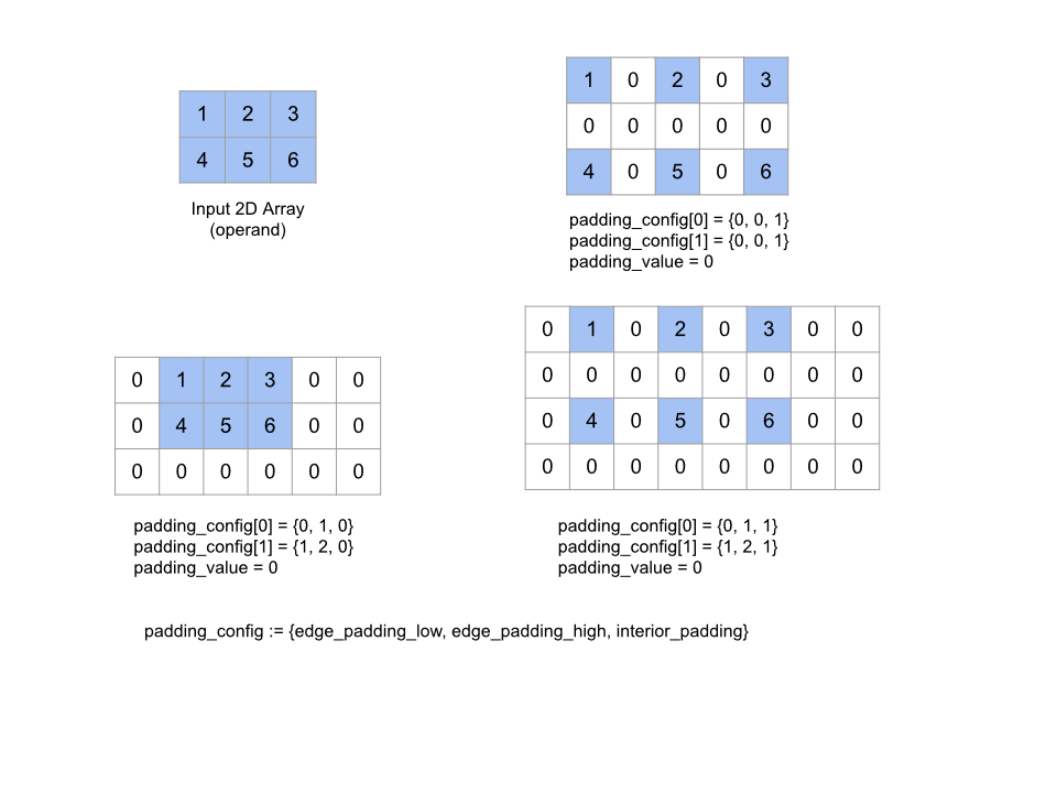
패드
XlaBuilder::Pad도 참고하세요.
Pad(operand, padding_value, padding_config)
| 인수 | 유형 | 시맨틱 |
|---|---|---|
operand |
XlaOp |
T 유형의 배열 |
padding_value |
XlaOp |
추가된 패딩을 채울 T 유형의 스칼라 |
padding_config |
PaddingConfig |
양쪽 가장자리 (낮음, 높음)와 각 크기의 요소 사이 패딩 값 |
지정된 padding_value가 있는 배열 주변과 배열 요소 사이의 패딩을 사용하여 지정된 operand 배열을 확장합니다. padding_config은 각 크기의 가장자리 패딩과 내부 패딩의 양을 지정합니다.
PaddingConfig는 PaddingConfigDimension의 반복되는 필드로, 각 측정기준에 edge_padding_low, edge_padding_high, interior_padding의 세 개의 필드가 포함되어 있습니다.
edge_padding_low와 edge_padding_high는 각 측정기준의 하위 값 (색인 0 옆)과 높은 값 (가장 높은 색인 옆)에 추가된 패딩의 양을 각각 지정합니다. 가장자리 패딩의 양은 음수일 수 있습니다. 음수 패딩의 절댓값은 지정된 크기에서 삭제할 요소의 수를 나타냅니다.
interior_padding은 각 차원에서 두 요소 사이에 추가되는 패딩의 양을 지정하며 음수가 아니어도 됩니다. 내부 패딩은 논리적으로 가장자리 패딩 전에 발생합니다. 따라서 음수 가장자리 패딩의 경우 내부 패딩 처리된 피연산자에서 요소가 삭제됩니다.
가장자리 패딩 쌍이 모두 (0, 0)이고 내부 패딩 값이 모두 0이면 이 연산은 작동하지 않습니다. 아래 그림은 2차원 배열의 다른 edge_padding 및 interior_padding 값의 예를 보여줍니다.
Recv
XlaBuilder::Recv도 참고하세요.
Recv(shape, channel_handle)
| 인수 | 유형 | 시맨틱 |
|---|---|---|
shape |
Shape |
수신하려는 데이터의 형태를 |
channel_handle |
ChannelHandle |
각 송수신 쌍에 대한 고유 식별자 |
같은 채널 핸들을 공유하는 다른 계산의 Send 명령에서 지정된 도형의 데이터를 수신합니다. 수신된 데이터의 XLOp를 반환합니다.
Recv 작업의 클라이언트 API는 동기 통신을 나타냅니다.
그러나 명령어는 내부적으로 2개의 HLO 명령(Recv 및 RecvDone)으로 분해되어 비동기 데이터 전송을 사용할 수 있습니다. HloInstruction::CreateRecv 및 HloInstruction::CreateRecvDone도 참고하세요.
Recv(const Shape& shape, int64 channel_id)
동일한 channel_id를 사용하여 Send 명령어에서 데이터를 수신하는 데 필요한 리소스를 할당합니다. 할당된 리소스의 컨텍스트를 반환하며, 다음 RecvDone 명령어에 의해 데이터 전송이 완료될 때까지 기다리는 데 사용됩니다. 컨텍스트는 {수신 버퍼 (셰이프), 요청 식별자(U32)}의 튜플이며 RecvDone 명령어에 의해서만 사용될 수 있습니다.
RecvDone(HloInstruction context)
Recv 명령어에 의해 생성된 컨텍스트가 주어지면 데이터 전송이 완료될 때까지 기다렸다가 수신된 데이터를 반환합니다.
방지(Reduce)
XlaBuilder::Reduce도 참고하세요.
축소 함수를 하나 이상의 배열에 동시에 적용합니다.
Reduce(operands..., init_values..., computation, dimensions)
| 인수 | 유형 | 시맨틱 |
|---|---|---|
operands |
N XlaOp의 시퀀스 |
T_0, ..., T_{N-1} 유형의 N 배열입니다. |
init_values |
N XlaOp의 시퀀스 |
T_0, ..., T_{N-1} 유형의 스칼라 N개 |
computation |
XlaComputation |
T_0, ..., T_{N-1}, T_0, ..., T_{N-1} -> Collate(T_0, ..., T_{N-1}) 유형의 계산 |
dimensions |
int64 배열 |
축소할 차원의 정렬되지 않은 배열입니다. |
각 항목의 의미는 다음과 같습니다.
- N은 1 이상이어야 합니다.
- 계산은 '대략적으로' 결합적이어야 합니다 (아래 참조).
- 모든 입력 배열은 차원이 동일해야 합니다.
- 모든 초깃값은
computation아래에서 ID를 형성해야 합니다. N = 1인 경우Collate(T)은T입니다.N > 1인 경우Collate(T_0, ..., T_{N-1})는T유형인N요소의 튜플입니다.
이 작업은 각 입력 배열의 차원 하나 이상을 스칼라로 줄입니다.
반환된 각 배열의 순위는 rank(operand) - len(dimensions)입니다. 작업의 출력은 Collate(Q_0, ..., Q_N)입니다. 여기서 Q_i는 T_i 유형의 배열이며 크기는 아래에 설명되어 있습니다.
서로 다른 백엔드에서 축소 계산을 다시 연결할 수 있습니다. 덧셈과 같은 일부 축소 함수는 부동 소수점 수와 결합되지 않으므로 숫자 차이가 발생할 수 있습니다. 그러나 데이터 범위가 제한적이면 부동 소수점 덧셈은 대부분의 실제 용도에서 결합될 만큼 충분합니다.
예
값이 [10, 11,
12, 13]인 단일 1차원 배열에서 한 차원을 축소하는 경우, 축소 함수 f (이는 computation)를 사용하여 다음과 같이 계산할 수 있습니다.
f(10, f(11, f(12, f(init_value, 13)))
다른 많은 가능성도 있습니다. 예를 들어
f(init_value, f(f(10, f(init_value, 11)), f(f(init_value, 12), f(init_value, 13))))
다음은 초깃값이 0인 축소 계산으로 합계를 사용하여 축소를 구현하는 방법을 보여주는 대략적인 의사 코드 예입니다.
result_shape <- remove all dims in dimensions from operand_shape

# Iterate over all elements in result_shape. The number of r's here is equal
# to the rank of the result
for r0 in range(result_shape[0]), r1 in range(result_shape[1]), ...:
  # Initialize this result element
  result[r0, r1...] <- 0

  # Iterate over all the reduction dimensions
  for d0 in range(dimensions[0]), d1 in range(dimensions[1]), ...:
    # Increment the result element with the value of the operand's element.
    # The index of the operand's element is constructed from all ri's and di's
    # in the right order (by construction ri's and di's together index over the
    # whole operand shape).
    result[r0, r1...] += operand[ri... di]
다음은 2D 배열 (행렬)을 줄이는 예입니다. 이 도형의 순위는 2, 차원 0은 크기 2, 차원 1은 크기 3입니다.
'add' 함수를 사용하여 차원 0 또는 1을 축소한 결과:
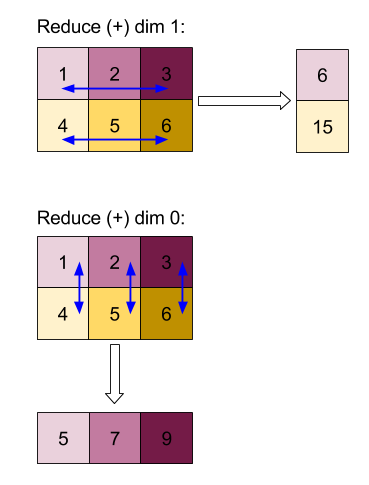
두 축소 결과는 모두 1차원 배열입니다. 이 다이어그램은 시각적 편의상 하나를 열로, 다른 하나를 행으로 보여줍니다.
더 복잡한 예는 3D 배열입니다. 순위는 3위, 차원 0은 크기 4, 차원 1은 크기가 2이고 차원 2는 3입니다. 편의상 값 1~6은 차원 0에 걸쳐 복제됩니다.
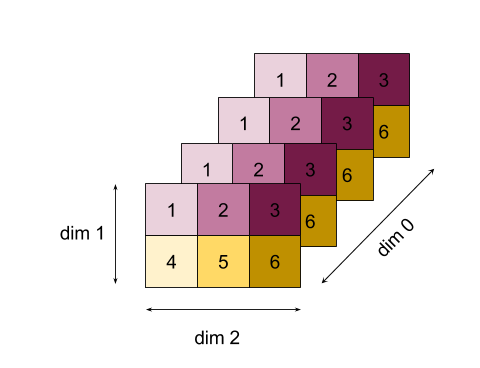
2D 예와 마찬가지로 1개의 차원만 줄일 수 있습니다. 예를 들어 차원 0을 줄이면 차원 0의 모든 값이 스칼라로 폴딩된 순위 2 배열이 생성됩니다.
|  4   8  12 |
| 16  20  24 |
차원 2를 줄이면 차원 2의 모든 값이 스칼라로 접힌 순위-2 배열도 생성됩니다.
| 6  15 |
| 6  15 |
| 6  15 |
| 6  15 |
입력의 나머지 차원 간의 상대적 순서는 출력에 보존되지만 일부 차원에는 새 숫자가 할당될 수 있습니다 (순위가 변경됨에 따라).
여러 측정기준을 줄일 수도 있습니다. 차원 0과 1을 더하면 1차원 배열 [20, 28, 36]이 생성됩니다.
모든 차원에서 3D 배열을 줄이면 스칼라 84가 생성됩니다.
Variadic 감소
N > 1인 경우 감소 함수 적용은 모든 입력에 동시에 적용되므로 약간 더 복잡합니다. 피연산자는 다음 순서로 계산에 제공됩니다.
- 첫 번째 피연산자의 감소된 값 실행
- ...
- N번째 피연산자의 감소된 값 실행
- 첫 번째 피연산자의 입력 값
- ...
- N번째 피연산자의 입력 값
예를 들어 1-D 배열의 최댓값과 argmax를 동시에 계산하는 데 사용할 수 있는 다음 축소 함수를 살펴보겠습니다.
f: (Float, Int, Float, Int) -> Float, Int
f(max, argmax, value, index):
  if value >= max:
    return (value, index)
  else:
    return (max, argmax)
1-D 입력 배열 V = Float[N], K = Int[N] 및 init 값 I_V = Float, I_K = Int의 경우 유일한 입력 차원에서 축소한 결과 f_(N-1)는 다음 재귀 적용과 동일합니다.
f_0 = f(I_V, I_K, V_0, K_0)
f_1 = f(f_0.first, f_0.second, V_1, K_1)
...
f_(N-1) = f(f_(N-2).first, f_(N-2).second, V_(N-1), K_(N-1))
이러한 축소를 값 배열과 순차 색인 배열 (즉, iota)에 적용하면 배열을 공동 반복하고 최대 값과 일치하는 색인을 포함하는 튜플이 반환됩니다.
ReducePrecision
XlaBuilder::ReducePrecision도 참고하세요.
부동 소수점 값을 정밀도가 낮은 형식 (예: IEEE-FP16)으로 변환하고 원래 형식으로 다시 변환하는 효과를 모델링합니다. 저정밀도 형식의 지수 및 가수 비트 수는 임의로 지정할 수 있지만, 일부 하드웨어 구현에서는 모든 비트 크기가 지원되지 않을 수도 있습니다.
ReducePrecision(operand, mantissa_bits, exponent_bits)
| 인수 | 유형 | 시맨틱 |
|---|---|---|
operand |
XlaOp |
부동 소수점 유형 T의 배열. |
exponent_bits |
int32 |
저정밀도 형식의 지수 비트 수 |
mantissa_bits |
int32 |
저정밀도 형식의 가수 비트 수 |
결과는 T 유형의 배열입니다. 입력 값은 주어진 가수 비트('짝수에 연결' 의미 체계를 사용)로 나타낼 수 있는 가장 가까운 값으로 반올림되며, 지수 비트 수로 지정된 범위를 초과하는 값은 양의 무한대 또는 음의 무한대로 고정됩니다. NaN 값은 유지되지만 표준 NaN 값으로 변환될 수 있습니다.
저정밀도 형식은 (0과 무한대 값을 구분하기 위해) 지수 비트가 하나 이상 있어야 하며(둘 다 가수 0이 있기 때문에) 음수가 아닌 수의 가수 비트를 가져야 합니다. 지수나 가수 비트의 수는 유형 T의 해당 값을 초과할 수 있습니다. 그러면 변환에서 상응하는 부분은 단순히 노옵스(no-ops)입니다.
ReduceScatter
XlaBuilder::ReduceScatter도 참고하세요.
ReduceScatter는 AllReduce를 효과적으로 실행한 다음 scatter_dimension와 함께 shard_count 블록으로 결과를 분할하여 결과를 분산하는 집합 작업으로, 복제본 그룹의 복제본 i가 ith 샤드를 수신합니다.
ReduceScatter(operand, computation, scatter_dim, shard_count,
replica_group_ids, channel_id)
| 인수 | 유형 | 시맨틱 |
|---|---|---|
operand |
XlaOp |
여러 복제본에서 줄일 배열 또는 비어 있지 않은 튜플입니다. |
computation |
XlaComputation |
감소 계산 |
scatter_dimension |
int64 |
분산할 측정기준입니다. |
shard_count |
int64 |
scatter_dimension 분할할 블록 수 |
replica_groups |
int64 벡터로 구성된 벡터 |
축소가 수행되는 그룹 |
channel_id |
선택사항 int64 |
교차 모듈 통신을 위한 채널 ID(선택사항) |
operand가 배열의 튜플이면 튜플의 각 요소에 감소-분산이 수행됩니다.replica_groups는 축소가 수행되는 복제본 그룹 목록입니다 (ReplicaId를 사용하여 현재 복제본의 복제본 ID를 가져올 수 있음). 각 그룹의 복제본 순서에 따라 All-Reduce 결과가 분산되는 순서가 결정됩니다.replica_groups은 비어 있거나 (이 경우 모든 복제본이 단일 그룹에 속함) 복제본 수와 동일한 수의 요소를 포함해야 합니다. 복제본 그룹이 2개 이상인 경우 모두 크기가 동일해야 합니다. 예를 들어replica_groups = {0, 2}, {1, 3}는0및2복제본과1및3간에 축소를 수행한 후 결과를 분산합니다.shard_count는 각 복제본 그룹의 크기입니다.replica_groups가 비어 있는 경우에 필요합니다.replica_groups가 비어 있지 않으면shard_count는 각 복제본 그룹의 크기와 동일해야 합니다.channel_id는 모듈 간 통신에 사용됩니다. 동일한channel_id가 있는reduce-scatter작업만 서로 통신할 수 있습니다.
출력 모양은 scatter_dimension를 shard_count배 더 작게 만든 입력 모양입니다. 예를 들어 복제본이 2개 있고 피연산자의 복제본 두 개에서 각각 [1.0, 2.25]과 [3.0, 5.25] 값이 있으면 scatter_dim이 0인 이 작업의 출력 값은 첫 번째 복제본은 [4.0]이고 두 번째 복제본은 [7.5]입니다.
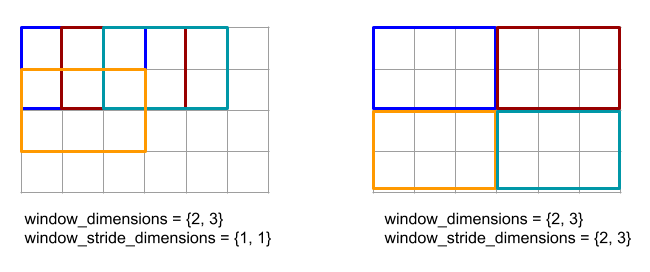
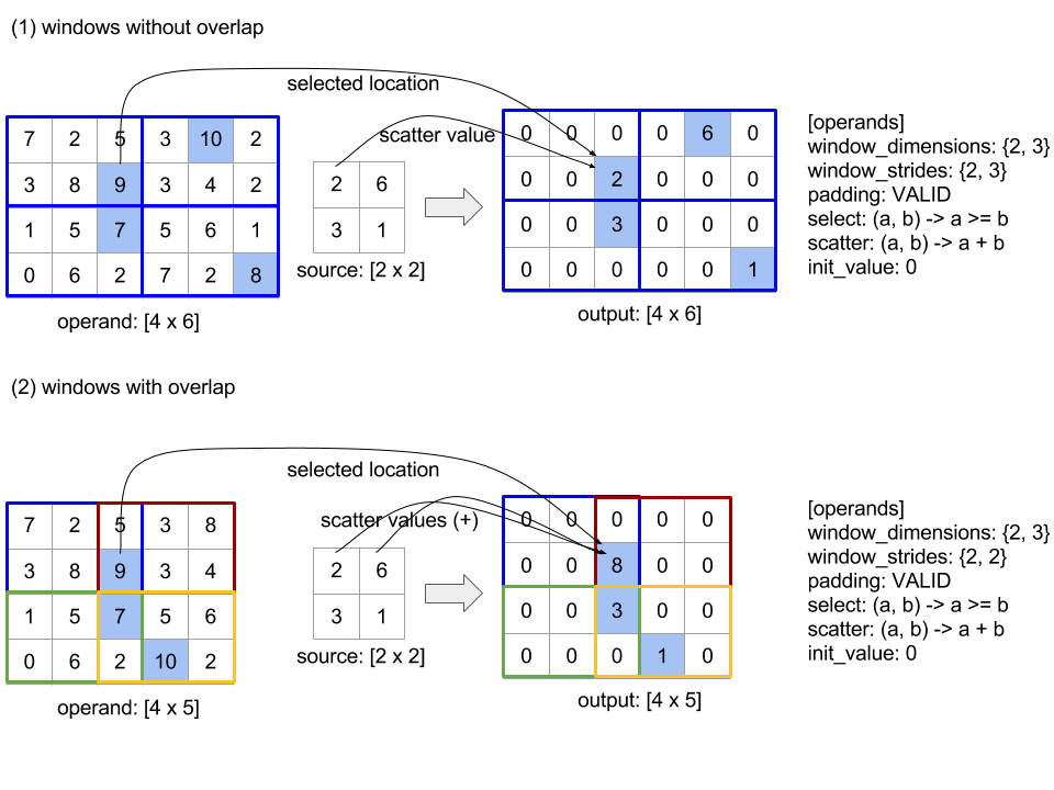
ReduceWindow
XlaBuilder::ReduceWindow도 참고하세요.
N개의 다차원 배열 시퀀스의 각 구간에 있는 모든 요소에 축소 함수를 적용하여 N개의 다차원 배열의 단일 또는 튜플을 출력으로 생성합니다. 각 출력 배열의 요소 수는 창의 유효한 위치 수와 동일합니다. 풀링 레이어는 ReduceWindow로 표현할 수 있습니다. Reduce와 마찬가지로 적용된 computation가 항상 왼쪽의 init_values에 전달됩니다.
ReduceWindow(operands..., init_values..., computation, window_dimensions,
window_strides, padding)
| 인수 | 유형 | 시맨틱 |
|---|---|---|
operands |
N XlaOps |
T_0,..., T_{N-1} 유형의 N 다차원 배열 시퀀스로, 각각 창이 배치된 기본 영역을 나타냅니다. |
init_values |
N XlaOps |
N개의 피연산자마다 하나씩, 축소를 위한 N개의 시작값. 자세한 내용은 축소를 참고하세요. |
computation |
XlaComputation |
모든 입력 피연산자의 각 윈도우에 있는 요소에 적용할 T_0, ..., T_{N-1}, T_0, ..., T_{N-1} -> Collate(T_0, ..., T_{N-1}) 유형의 감소 함수입니다. |
window_dimensions |
ArraySlice<int64> |
기간 측정기준 값의 정수 배열 |
window_strides |
ArraySlice<int64> |
윈도우 스트라이드 값의 정수 배열 |
base_dilations |
ArraySlice<int64> |
염기 확장 값의 정수 배열 |
window_dilations |
ArraySlice<int64> |
창 확장 값의 정수 배열 |
padding |
Padding |
창의 패딩 유형 (스트라이드가 1인 경우 입력과 동일한 출력 셰이프를 갖도록 패딩하는 Padding::kSame, 패딩을 사용하지 않고 더 이상 맞지 않으면 창을 '중지'함) |
각 항목의 의미는 다음과 같습니다.
- N은 1 이상이어야 합니다.
- 모든 입력 배열은 차원이 동일해야 합니다.
N = 1인 경우Collate(T)은T입니다.N > 1인 경우Collate(T_0, ..., T_{N-1})는(T0,...T{N-1})유형인N요소의 튜플입니다.
아래 코드와 그림은 ReduceWindow를 사용하는 예를 보여줍니다. 입력은 [4x6] 크기의 행렬이며 window_dimensions와 window_stride_dimensions는 [2x3]입니다.
// Create a computation for the reduction (maximum).
XlaComputation max;
{
  XlaBuilder builder(client_, "max");
  auto y = builder.Parameter(0, ShapeUtil::MakeShape(F32, {}), "y");
  auto x = builder.Parameter(1, ShapeUtil::MakeShape(F32, {}), "x");
  builder.Max(y, x);
  max = builder.Build().value();
}

// Create a ReduceWindow computation with the max reduction computation.
XlaBuilder builder(client_, "reduce_window_2x3");
auto shape = ShapeUtil::MakeShape(F32, {4, 6});
auto input = builder.Parameter(0, shape, "input");
builder.ReduceWindow(
    input,
    /*init_val=*/builder.ConstantLiteral(LiteralUtil::MinValue(F32)),
    *max,
    /*window_dimensions=*/{2, 3},
    /*window_stride_dimensions=*/{2, 3},
    Padding::kValid);
측정기준의 스트라이드가 1이면 크기 내 창의 위치가 인접한 창에서 요소 1개 떨어진 위치에 있음을 나타냅니다. 기간이 서로 겹치지 않도록 지정하려면 window_stride_dimensions는 window_dimensions와 같아야 합니다. 아래 그림은 서로 다른 두 스트라이드 값을 사용하는 방법을 보여줍니다. 패딩은 입력의 각 차원에 적용되며, 패딩 후에 입력에 차원이 적용된 것과 계산이 같습니다.
중요한 패딩의 경우 입력 배열 [10000, 1000, 100, 10, 1]에 대해 차원 3과 스트라이드 2를 사용하여 감소 기간 최솟값(초기값은 MAX_FLOAT)을 계산해 보세요. 패딩 kValid는 두 개의 유효한 기간([10000, 1000, 100] 및 [100, 10, 1])에 걸쳐 최솟값을 계산하므로 [100, 1] 출력이 생성됩니다. 패딩 kSame는 먼저 배열을 패딩하여 축소 창 이후의 도형이 양쪽에 초기 요소를 추가하고 [MAX_VALUE, 10000, 1000, 100, 10, 1,
MAX_VALUE]를 가져와 스트라이드 1의 입력과 동일하도록 합니다. 패딩된 배열에 대해Reduce-window를 실행하는 것은 3개의 창 [MAX_VALUE, 10000, 1000], [1000, 100, 10], [10, 1, MAX_VALUE], 수익 [1000, 10, 1]에서 작동합니다.
축소 함수의 평가 순서는 임의적이며 비확정적일 수 있습니다. 따라서 축소 함수는 재연결에 지나치게 민감하지 않아야 합니다. 자세한 내용은 Reduce 컨텍스트에서의 연결성에 관한 설명을 참고하세요.
ReplicaId
XlaBuilder::ReplicaId도 참고하세요.
복제본의 고유 ID (U32 스칼라)를 반환합니다.
ReplicaId()
각 복제본의 고유 ID는 [0, N) 간격의 부호 없는 정수입니다. 여기서 N는 복제본 수입니다. 모든 복제본이 동일한 프로그램을 실행하므로 프로그램에서 ReplicaId()을 호출하면 각 복제본에 다른 값이 반환됩니다.
재구성
XlaBuilder::Reshape 및 Collapse 작업도 참고하세요.
배열의 차원을 새 구성으로 다시 만듭니다.
Reshape(operand, new_sizes)
Reshape(operand, dimensions, new_sizes)
| 인수 | 유형 | 시맨틱 |
|---|---|---|
operand |
XlaOp |
유형 T의 배열 |
dimensions |
int64 벡터 |
크기가 축소되는 순서 |
new_sizes |
int64 벡터 |
새 차원의 크기의 벡터 |
개념적으로 형태를 바꾸려면 먼저 배열을 데이터 값의 1차원 벡터로 평면화한 다음 이 벡터를 새로운 모양으로 미세 조정합니다. 입력 인수는 T 유형의 임의 배열, 차원 색인의 컴파일 시간 상수 벡터, 결과의 차원 크기의 컴파일 시간 상수 벡터입니다.
dimension 벡터의 값은 지정된 경우 모든 T 차원의 순열이어야 합니다. 지정되지 않은 경우 기본값은 {0, ..., rank - 1}입니다. dimensions의 차원 순서는 입력 배열을 단일 차원으로 축소하는 루프 중첩에서 가장 느리게 변하는 차원 (가장 주요한 차원)부터 가장 빠르게 변화하는 차원 (가장 작은 차원)까지입니다. new_sizes 벡터는 출력 배열의 크기를 결정합니다. new_sizes에서 색인 0에 있는 값은 측정기준 0의 크기이고 색인 1의 값은 측정기준 1의 크기입니다. new_size 측정기준의 곱은 피연산자의 측정기준 크기를 곱한 값과 같아야 합니다. 축소된 배열을 new_sizes로 정의된 다차원 배열로 미세 조정할 때 new_sizes의 차원은 가장 느린 차원 (가장 큰 차이)부터 가장 빠른 차원 (가장 작은 값) 순으로 정렬됩니다.
예를 들어 v를 24개 요소의 배열이라고 가정해 보겠습니다.
let v = f32[4x2x3] { { {10, 11, 12}, {15, 16, 17} },
                    { {20, 21, 22}, {25, 26, 27} },
                    { {30, 31, 32}, {35, 36, 37} },
                    { {40, 41, 42}, {45, 46, 47} } };

In-order collapse:
let v012_24 = Reshape(v, {0,1,2}, {24});
then v012_24 == f32[24] {10, 11, 12, 15, 16, 17, 20, 21, 22, 25, 26, 27,
                         30, 31, 32, 35, 36, 37, 40, 41, 42, 45, 46, 47};

let v012_83 = Reshape(v, {0,1,2}, {8,3});
then v012_83 == f32[8x3] { {10, 11, 12}, {15, 16, 17},
                          {20, 21, 22}, {25, 26, 27},
                          {30, 31, 32}, {35, 36, 37},
                          {40, 41, 42}, {45, 46, 47} };

Out-of-order collapse:
let v021_24 = Reshape(v, {1,2,0}, {24});
then v012_24 == f32[24]  {10, 20, 30, 40, 11, 21, 31, 41, 12, 22, 32, 42,
                          15, 25, 35, 45, 16, 26, 36, 46, 17, 27, 37, 47};

let v021_83 = Reshape(v, {1,2,0}, {8,3});
then v021_83 == f32[8x3] { {10, 20, 30}, {40, 11, 21},
                          {31, 41, 12}, {22, 32, 42},
                          {15, 25, 35}, {45, 16, 26},
                          {36, 46, 17}, {27, 37, 47} };


let v021_262 = Reshape(v, {1,2,0}, {2,6,2});
then v021_262 == f32[2x6x2] { { {10, 20}, {30, 40},
                              {11, 21}, {31, 41},
                              {12, 22}, {32, 42} },
                             { {15, 25}, {35, 45},
                              {16, 26}, {36, 46},
                              {17, 27}, {37, 47} } };
특수한 사례로 형태를 변경하면 단일 요소 배열을 스칼라로 변환하거나 그 반대로 변환할 수 있습니다. 예를 들면 다음과 같습니다.
Reshape(f32[1x1] { {5} }, {0,1}, {}) == 5;
Reshape(5, {}, {1,1}) == f32[1x1] { {5} };
수익 (역순)
XlaBuilder::Rev도 참고하세요.
Rev(operand, dimensions)
| 인수 | 유형 | 시맨틱 |
|---|---|---|
operand |
XlaOp |
유형 T의 배열 |
dimensions |
ArraySlice<int64> |
거꾸로 된 측정기준 |
지정된 dimensions에 따라 operand 배열에 있는 요소의 순서를 반대로 전환하여 동일한 모양의 출력 배열을 생성합니다. 다차원 색인에서 피연산자 배열의 각 요소는 변환된 색인의 출력 배열에 저장됩니다. 다차원 색인은 각 측정기준의 색인을 반대로 반전하여 변환됩니다. 즉, 크기 N의 차원이 역방향 차원 중 하나인 경우 색인 i가 N - 1 - i로 변환됩니다.
Rev 연산의 한 가지 용도는 신경망의 기울기 계산 중에 두 기간 차원에 따라 컨볼루션 가중치 배열을 역전시키는 것입니다.
RngNormal
XlaBuilder::RngNormal도 참고하세요.
\(N(\mu, \sigma)\) 정규 분포에 따라 생성된 난수를 사용하여 특정 도형의 출력을 생성합니다. 매개변수 \(\mu\) , \(\sigma\), 출력 도형은 부동 소수점 요소 유형이어야 합니다. 또한 매개변수는 스칼라 값이어야 합니다.
RngNormal(mu, sigma, shape)
| 인수 | 유형 | 시맨틱 |
|---|---|---|
mu |
XlaOp |
생성된 숫자의 평균을 지정하는 T 유형의 스칼라 |
sigma |
XlaOp |
생성된 표준 편차를 지정하는 T 유형의 스칼라 |
shape |
Shape |
유형 T의 출력 셰이프 |
RngUniform
XlaBuilder::RngUniform도 참고하세요.
간격 \([a,b)\)에 걸쳐 균일한 분포를 따라 생성된 난수를 사용하여 지정된 도형의 출력을 생성합니다. 매개변수와 출력 요소 유형은 불리언 유형, 정수 유형 또는 부동 소수점 유형이어야 하며 유형은 일관되어야 합니다. CPU 및 GPU 백엔드는 현재 F64, F32, F16, BF16, S64, U64, S32, U32만 지원합니다. 또한 매개변수는 스칼라 값이어야 합니다. \(b <= a\) 인 경우 결과는 구현으로 정의됩니다.
RngUniform(a, b, shape)
| 인수 | 유형 | 시맨틱 |
|---|---|---|
a |
XlaOp |
간격의 하한을 지정하는 T 유형의 스칼라 |
b |
XlaOp |
간격의 상한을 지정하는 T 유형의 스칼라 |
shape |
Shape |
유형 T의 출력 셰이프 |
RngBitGenerator
지정된 알고리즘 (또는 백엔드 기본값)을 사용하여 균일한 임의의 비트로 채워진 지정된 도형으로 출력을 생성하고 업데이트된 상태 (초기 상태와 동일한 형태) 및 생성된 무작위 데이터를 반환합니다.
초기 상태는 현재 랜덤 숫자 생성의 초기 상태입니다. 이 함수와 필요한 형태 및 유효한 값은 사용되는 알고리즘에 따라 다릅니다.
출력은 초기 상태의 확정적 함수가 보장되지만 백엔드와 다른 컴파일러 버전 간에 확정성이 보장되지는 않습니다.
RngBitGenerator(algorithm, key, shape)
| 인수 | 유형 | 시맨틱 |
|---|---|---|
algorithm |
RandomAlgorithm |
사용됩니다. |
initial_state |
XlaOp |
PRNG 알고리즘의 초기 상태입니다. |
shape |
Shape |
생성된 데이터의 출력 셰이프 |
사용 가능한 algorithm 값:
rng_default: 백엔드별 형태 요구사항이 있는 백엔드별 알고리즘입니다.rng_three_fry: ThreeFry 카운터 기반 PRNG 알고리즘입니다.initial_state모양은 임의의 값을 가진u64[2]입니다. Salmon 외 SC 2011년. 병렬 랜덤 숫자: 1, 2, 3만큼 간단합니다.rng_philox: 랜덤 숫자를 동시에 생성하는 Philox 알고리즘입니다.initial_state도형은 임의의 값이 있는u64[3]입니다. Salmon 외 SC 2011년. 병렬 랜덤 숫자: 1, 2, 3만큼 간단합니다.
분산형
XLA 분산형 연산은 update_computation를 사용하여 updates의 값 시퀀스로 업데이트된 여러 슬라이스 (scatter_indices로 지정된 색인에서)가 있는 입력 배열 operands의 값인 결과 시퀀스를 생성합니다.
XlaBuilder::Scatter도 참고하세요.
scatter(operands..., scatter_indices, updates..., update_computation,
index_vector_dim, update_window_dims, inserted_window_dims,
scatter_dims_to_operand_dims)
| 인수 | 유형 | 시맨틱 |
|---|---|---|
operands |
N XlaOp의 시퀀스 |
분산될 T_0, ..., T_N 유형의 N 배열입니다. |
scatter_indices |
XlaOp |
분산해야 하는 슬라이스의 시작 색인이 포함된 배열입니다. |
updates |
N XlaOp의 시퀀스 |
T_0, ..., T_N 유형의 N 배열입니다. updates[i]에는 operands[i]를 분산하는 데 사용해야 하는 값이 포함됩니다. |
update_computation |
XlaComputation |
입력 배열의 기존 값과 분산 중에 업데이트를 결합하는 데 사용되는 계산입니다. 이 계산은 T_0, ..., T_N, T_0, ..., T_N -> Collate(T_0, ..., T_N) 유형이어야 합니다. |
index_vector_dim |
int64 |
시작 색인이 포함된 scatter_indices의 측정기준입니다. |
update_window_dims |
ArraySlice<int64> |
updates 도형의 창 크기인 크기 집합입니다. |
inserted_window_dims |
ArraySlice<int64> |
updates 도형에 삽입해야 하는 창 크기 집합입니다. |
scatter_dims_to_operand_dims |
ArraySlice<int64> |
분산형 색인에서 피연산자 색인 공간으로 차원이 매핑됩니다. 이 배열은 i를 scatter_dims_to_operand_dims[i]에 매핑하는 것으로 해석됩니다 . 일대일로 진행되어야 합니다. |
indices_are_sorted |
bool |
호출자에 의한 색인 정렬이 보장되는지 여부입니다. |
각 항목의 의미는 다음과 같습니다.
- N은 1 이상이어야 합니다.
operands[0], ...,operands[N-1] 은(는) 모두 크기가 동일해야 합니다.updates[0], ...,updates[N-1] 은(는) 모두 크기가 동일해야 합니다.N = 1인 경우Collate(T)은T입니다.N > 1인 경우Collate(T_0, ..., T_N)는T유형의N요소의 튜플입니다.
index_vector_dim이 scatter_indices.rank와 같으면 scatter_indices에 후행 1 차원이 있는 것으로 암시적으로 간주합니다.
ArraySlice<int64> 유형의 update_scatter_dims를 update_window_dims이 아닌 updates 도형의 치수 집합으로 오름차순으로 정의합니다.
scatter 인수는 다음 제약 조건을 따라야 합니다.
각
updates배열은 순위가update_window_dims.size + scatter_indices.rank - 1이어야 합니다.각
updates배열에서i측정기준의 경계는 다음을 준수해야 합니다.i가update_window_dims에 존재하는 경우 (즉, 일부k의 경우update_window_dims[k])updates의 측정기준i경계는inserted_window_dims를 고려한 후 해당operand의 경계를 초과하면 안 됩니다 (즉,adjusted_window_bounds[k]. 여기서adjusted_window_bounds은operand의 경계가 포함되고 색인inserted_window_dims의 경계가 삭제된 경우).i가update_scatter_dims에 있는 경우 (즉, 일부k의 경우update_scatter_dims[k])updates의i측정기준 경계는index_vector_dim를 건너뛰는scatter_indices의 해당 경계와 동일해야 합니다 (즉,k<index_vector_dim이면scatter_indices.shape.dims[k], 그렇지 않으면scatter_indices.shape.dims[k+1]).
update_window_dims은(는) 오름차순이어야 하고 반복되는 측정기준 숫자가 없어야 하며[0, updates.rank)범위 내에 있어야 합니다.inserted_window_dims은(는) 오름차순이어야 하고 반복되는 측정기준 숫자가 없어야 하며[0, operand.rank)범위 내에 있어야 합니다.operand.rank는update_window_dims.size와inserted_window_dims.size의 합과 같아야 합니다.scatter_dims_to_operand_dims.size는scatter_indices.shape.dims[index_vector_dim]와 같아야 하고 값은[0, operand.rank)범위 내에 있어야 합니다.
각 updates 배열의 특정 색인 U의 경우 이 업데이트를 적용해야 하는 상응하는 operands 배열의 해당 색인 I은 다음과 같이 계산됩니다.
update_scatter_dims의k에 대해G= {U[k] 입니다.G를 사용하여scatter_indices배열에서 인덱스 벡터S를 조회하여S[i] =scatter_indices[합성(G,i)] 을 할 수 있습니다. 여기서 결합(A, b)은 위치index_vector_dim에 b를 A에 삽입합니다.scatter_dims_to_operand_dims맵으로S를 분산하여S를 사용하여operand에 색인Sin을 만듭니다. 더 공식적으로 다음과 같이 표기합니다.Sin[scatter_dims_to_operand_dims[k]] =S[k] ifk<scatter_dims_to_operand_dims.size.Sin[_] =0(그렇지 않은 경우)
inserted_window_dims에 따라U의update_window_dims에 색인을 분산하여 각operands배열에 색인Win를 만듭니다. 더 공식적으로 다음과 같이 표기합니다.k가update_window_dims에 있는 경우Win[window_dims_to_operand_dims(k)] =U[k]. 여기서window_dims_to_operand_dims는 도메인 [0,update_window_dims.size) 및 범위가 [0,operand.rank) \inserted_window_dims인 단조 함수입니다. 예를 들어update_window_dims.size이4,operand.rank가6,inserted_window_dims가 {0,2}이면window_dims_to_operand_dims는 {0→1,1→3,2→4,3→5}입니다.Win[_] =0(그렇지 않은 경우)
I는Win+Sin이며, 여기서 +는 요소별 덧셈입니다.
분산 작업은 다음과 같이 정의할 수 있습니다.
operands를 사용하여output를 초기화합니다.즉, 모든 색인J의 경우operands[J] 배열의 모든 색인O에 대해 다음과 같이 초기화합니다.
output[J][O] =operands[J][O]updates[J] 배열의 색인U및operand[J] 배열의 해당 색인O에 대해O이 유효한 색인인 경우:
(output[0][O], ...,output[N-1][O]) =update_computation(output[0][O], ..., ,output[N-1][O],updates[0][U], ...,updates[N-1][U])output
업데이트가 적용되는 순서는 비확정적입니다. 따라서 updates의 여러 색인이 operands의 동일한 색인을 참조하는 경우 output의 상응하는 값은 비확정적입니다.
update_computation에 전달되는 첫 번째 매개변수는 항상 output 배열의 현재 값이고 두 번째 매개변수는 항상 updates 배열의 값입니다. 이는 update_computation가 가환 법칙이 아닌 경우에 특히 중요합니다.
indices_are_sorted이 true로 설정된 경우 XLA는 사용자가 start_indices를 오름차순 (start_index_map의 오름차순)으로 정렬한다고 가정할 수 있습니다. 그렇지 않으면 시맨틱이 구현됩니다.
분산 작업은 비공식적으로 수집 작업의 반대로 볼 수 있습니다. 즉, 분산 작업은 해당 수집 작업에서 추출된 입력의 요소를 업데이트합니다.
비공식적인 설명과 예시는 Gather의 '구어체 설명' 섹션을 참고하세요.
선택
XlaBuilder::Select도 참고하세요.
조건자 배열의 값을 기준으로 두 입력 배열의 요소에서 출력 배열을 생성합니다.
Select(pred, on_true, on_false)
| 인수 | 유형 | 시맨틱 |
|---|---|---|
pred |
XlaOp |
PRED 유형의 배열 |
on_true |
XlaOp |
유형 T의 배열 |
on_false |
XlaOp |
유형 T의 배열 |
on_true 및 on_false 배열은 형태가 동일해야 합니다. 이는 출력 배열의
형태이기도 합니다. pred 배열은 on_true 및 on_false와 차원이 같고 요소 유형이 PRED여야 합니다.
pred의 각 요소 P의 경우 출력 배열의 상응하는 요소는 P 값이 true이면 on_true에서, P 값이 false이면 on_false에서 가져옵니다. 제한된 형태의 브로드캐스트로서 pred는 PRED 유형의 스칼라일 수 있습니다. 이 경우 출력 배열은 pred가 true이면 on_true에서, pred가 false이면 on_false에서 완전히 가져옵니다.
비스칼라 pred 사용 예:
let pred: PRED[4] = {true, false, false, true};
let v1: s32[4] = {1, 2, 3, 4};
let v2: s32[4] = {100, 200, 300, 400};
==>
Select(pred, v1, v2) = s32[4]{1, 200, 300, 4};
스칼라 pred 사용 예시:
let pred: PRED = true;
let v1: s32[4] = {1, 2, 3, 4};
let v2: s32[4] = {100, 200, 300, 400};
==>
Select(pred, v1, v2) = s32[4]{1, 2, 3, 4};
튜플 간의 선택이 지원됩니다. 이를 위해 튜플은 스칼라 유형으로 간주됩니다. on_true 및 on_false가 튜플 (동일한 형태를 가져야 함)이면 pred는 PRED 유형의 스칼라여야 합니다.
SelectAndScatter
XlaBuilder::SelectAndScatter도 참고하세요.
이 연산은 먼저 operand 배열에서 ReduceWindow을 계산하여 각 윈도우에서 요소를 선택한 후 source 배열을 선택된 요소의 색인에 분산하여 피연산자 배열과 형태가 동일한 출력 배열을 생성하는 복합 연산으로 간주될 수 있습니다. 바이너리 select 함수는 각 윈도우에 걸쳐 요소를 적용하여 각 윈도우에서 요소를 선택하는 데 사용되며, 첫 번째 매개변수의 색인 벡터가 두 번째 매개변수의 색인 벡터보다 사전순으로 작다는 속성으로 호출됩니다. select 함수는 첫 번째 매개변수가 선택되면 true를 반환하고 두 번째 매개변수가 선택되면 false를 반환하며, 함수는 전이성을 유지해야 합니다 (즉, select(a, b)와 select(b, c)가 true이면 select(a, c)도 true임). 그래야 선택된 요소가 지정된 기간 동안 순회하는 요소의 순서에 종속되지 않습니다.
scatter 함수는 출력 배열에서 선택된 각 색인에 적용됩니다. 스칼라 매개변수 두 개를 사용합니다.
- 출력 배열에서 선택된 색인의 현재 값
- 선택한 색인에 적용되는
source의 분산형 값입니다.
이 함수는 두 매개변수를 결합하고 출력 배열에서 선택된 색인의 값을 업데이트하는 데 사용되는 스칼라 값을 반환합니다. 처음에는 출력 배열의 모든 색인이 init_value로 설정됩니다.
출력 배열은 operand 배열과 형태가 같으며 source 배열은 operand 배열에 ReduceWindow 연산을 적용한 결과와 형태가 동일해야 합니다. SelectAndScatter는 신경망에서 풀링 레이어의 경사 값을 역전파하는 데 사용할 수 있습니다.
SelectAndScatter(operand, select, window_dimensions, window_strides,
padding, source, init_value, scatter)
| 인수 | 유형 | 시맨틱 |
|---|---|---|
operand |
XlaOp |
창이 슬라이드되는 T 유형의 배열 |
select |
XlaComputation |
각 기간의 모든 요소에 적용할 T, T -> PRED 유형의 바이너리 계산. 첫 번째 매개변수를 선택하면 true를 반환하고 두 번째 매개변수를 선택하면 false을 반환합니다. |
window_dimensions |
ArraySlice<int64> |
기간 측정기준 값의 정수 배열 |
window_strides |
ArraySlice<int64> |
윈도우 스트라이드 값의 정수 배열 |
padding |
Padding |
창의 패딩 유형 (Padding::kSame 또는 Padding::kValid) |
source |
XlaOp |
분산할 값이 있는 T 유형의 배열 |
init_value |
XlaOp |
출력 배열의 초깃값으로 T 유형의 스칼라 값 |
scatter |
XlaComputation |
T, T -> T 유형의 바이너리 계산: 각 분산형 소스 요소를 대상 요소와 함께 적용 |
아래 그림은 매개변수 중 최대값을 계산하는 select 함수와 함께 SelectAndScatter를 사용하는 예를 보여줍니다. 아래 그림 (2)와 같이 기간이 겹치는 경우 서로 다른 기간에 의해 operand 배열의 색인이 여러 번 선택될 수 있습니다. 이 그림에서 값 9의 요소는 맨 위 창 (파란색 및 빨간색)에 의해 선택되고, 바이너리 더하기 scatter 함수는 값 8 (2 + 6)의 출력 요소를 생성합니다.
scatter 함수의 평가 순서는 임의적이며 비확정적일 수 있습니다. 따라서 scatter 함수는 재연결에 지나치게 민감하지 않아야 합니다. 자세한 내용은 Reduce 컨텍스트에서의 연결성에 관한 설명을 참고하세요.
보내기
XlaBuilder::Send도 참고하세요.
Send(operand, channel_handle)
| 인수 | 유형 | 시맨틱 |
|---|---|---|
operand |
XlaOp |
전송할 데이터 (T 유형 배열) |
channel_handle |
ChannelHandle |
각 송수신 쌍에 대한 고유 식별자 |
지정된 피연산자 데이터를 동일한 채널 핸들을 공유하는 다른 계산의 Recv 명령어로 전송합니다. 데이터를 반환하지 않습니다.
Recv 작업과 마찬가지로 Send 작업의 클라이언트 API는 동기 통신을 나타내며 비동기 데이터 전송을 사용 설정하도록 내부적으로 2개의 HLO 명령(Send 및 SendDone)으로 분해됩니다. HloInstruction::CreateSend 및 HloInstruction::CreateSendDone도 참고하세요.
Send(HloInstruction operand, int64 channel_id)
동일한 채널 ID를 가진 Recv 명령어에 의해 할당된 리소스로 피연산자의 비동기 전송을 시작합니다. 데이터 전송이 완료될 때까지 기다리기 위해 다음 SendDone 명령어에 의해 사용되는 컨텍스트를 반환합니다. 컨텍스트는 {피연산자 (모양), 요청 식별자(U32)}의 튜플이며 SendDone 명령에서만 사용할 수 있습니다.
SendDone(HloInstruction context)
Send 명령어에 의해 생성된 컨텍스트가 주어지면 데이터 전송이 완료될 때까지 기다립니다. 명령이 데이터를 반환하지 않습니다.
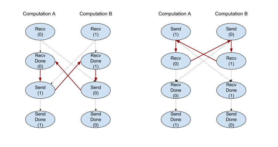
채널 지침 일정 예약
각 채널 (Recv, RecvDone, Send, SendDone)에 관한 명령어 4개의 실행 순서는 다음과 같습니다.
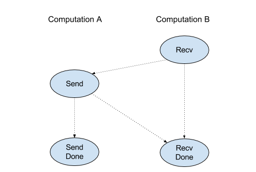
Recv은(는)Send전에 발생합니다.Send은(는)RecvDone전에 발생합니다.Recv은(는)RecvDone전에 발생합니다.Send은(는)SendDone전에 발생합니다.
백엔드 컴파일러가 채널 명령을 통해 통신하는 각 계산에 대해 선형 일정을 생성할 때 계산 과정이 반복되어서는 안 됩니다. 예를 들어 아래 일정은 교착 상태를 유발합니다.
슬라이스
XlaBuilder::Slice도 참고하세요.
슬라이싱은 입력 배열에서 하위 배열을 추출합니다. 하위 배열은 입력과 순위가 같으며 경계 상자의 크기와 색인이 슬라이스 연산의 인수로 주어지는 입력 배열 내의 경계 상자 안에 있는 값을 포함합니다.
Slice(operand, start_indices, limit_indices, strides)
| 인수 | 유형 | 시맨틱 |
|---|---|---|
operand |
XlaOp |
유형 T의 N차원 배열 |
start_indices |
ArraySlice<int64> |
각 차원에 대한 슬라이스의 시작 색인을 포함하는 N개의 정수 목록입니다. 값은 0 이상이어야 합니다. |
limit_indices |
ArraySlice<int64> |
각 차원의 슬라이스에 대해 끝 색인 (제외)을 포함하는 N개의 정수 목록입니다. 각 값은 크기의 각 start_indices 값보다 크거나 같아야 하고 크기보다 작거나 같아야 합니다. |
strides |
ArraySlice<int64> |
슬라이스의 입력 스트라이드를 결정하는 N개의 정수 목록입니다. 슬라이스는 측정기준 d에서 모든 strides[d] 요소를 선택합니다. |
1차원 예:
let a = {0.0, 1.0, 2.0, 3.0, 4.0}
Slice(a, {2}, {4}) produces:
  {2.0, 3.0}
2차원 예:
let b =
 { {0.0,  1.0,  2.0},
   {3.0,  4.0,  5.0},
   {6.0,  7.0,  8.0},
   {9.0, 10.0, 11.0} }

Slice(b, {2, 1}, {4, 3}) produces:
  { { 7.0,  8.0},
    {10.0, 11.0} }
정렬
XlaBuilder::Sort도 참고하세요.
Sort(operands, comparator, dimension, is_stable)
| 인수 | 유형 | 시맨틱 |
|---|---|---|
operands |
ArraySlice<XlaOp> |
정렬할 피연산자입니다. |
comparator |
XlaComputation |
사용할 비교 연산자 계산입니다. |
dimension |
int64 |
정렬할 측정기준입니다. |
is_stable |
bool |
안정적 정렬의 사용 여부입니다. |
피연산자가 하나만 제공된 경우:
피연산자가 rank-1 텐서 (배열)인 경우 결과는 정렬된 배열입니다. 배열을 오름차순으로 정렬하려면 비교 연산자가 보다 작음 비교를 수행해야 합니다. 배열이 정렬된 후에는
i < j가comparator(value[i], value[j]) = comparator(value[j], value[i]) = false또는comparator(value[i], value[j]) = true인 모든 색인 위치i, j에 대해 배열이 유지됩니다.피연산자의 순위가 더 높으면 제공된 측정기준을 따라 피연산자가 정렬됩니다. 예를 들어 rank-2 텐서 (행렬)의 경우 측정기준 값
0은 모든 열을 독립적으로 정렬하고 측정기준 값1는 각 행을 독립적으로 정렬합니다. 측정기준 번호를 입력하지 않으면 기본적으로 마지막 측정기준이 선택됩니다. 정렬된 측정기준의 경우 순위-1 사례와 동일한 정렬 순서가 적용됩니다.
n > 1 피연산자가 제공된 경우:
모든
n피연산자는 동일한 차원의 텐서여야 합니다. 텐서의 요소 유형은 다를 수 있습니다.모든 피연산자가 개별적으로 정렬되지 않고 함께 정렬됩니다. 개념적으로 피연산자는 튜플로 취급됩니다. 색인 위치
i와j에 있는 각 피연산자의 요소를 교체해야 하는지 확인할 때 비교 연산자는2 * n스칼라 매개변수로 호출됩니다. 여기서 매개변수2 * k는k-th피연산자의i위치에 있는 값에 상응하고 매개변수2 * k + 1는k-th피연산자의j위치에 있는 값에 상응합니다. 따라서 일반적으로 비교자는2 * k및2 * k + 1매개변수를 서로 비교하며 다른 매개변수 쌍을 연결 고리로 사용할 수 있습니다.결과는 정렬된 순서로 피연산자 (위와 같이 제공된 측정기준)로 구성된 튜플입니다. 튜플의
i-th피연산자는 Sort의i-th피연산자에 상응합니다.
예를 들어 세 개의 피연산자 operand0 = [3, 1], operand1 = [42, 50], operand2 = [-3.0, 1.1]가 있고 비교 연산자는 operand0의 값만 보다 작음과 비교하면 정렬의 출력은 ([1, 3], [50, 42], [1.1, -3.0]) 튜플입니다.
is_stable를 true로 설정하면 정렬이 안정적으로 이루어집니다. 즉, 비교 연산자에 의해 동일한 것으로 간주되는 요소가 있는 경우 동일한 값의 상대적 순서가 유지됩니다. 두 요소 e1와 e2는 comparator(e1, e2) = comparator(e2, e1) = false인 경우에만 동일합니다. 기본적으로 is_stable은 false로 설정됩니다.
전치행렬
tf.reshape 작업도 참고하세요.
Transpose(operand)
| 인수 | 유형 | 시맨틱 |
|---|---|---|
operand |
XlaOp |
전치할 피연산자입니다. |
permutation |
ArraySlice<int64> |
크기를 순열하는 방법 |
지정된 순열로 피연산자 측정기준을 순열합니다. 즉, ∀ i . 0 ≤ i < rank ⇒ input_dimensions[permutation[i]] = output_dimensions[i]입니다.
Reshape(피연산자, 순열, Permute(per 뮤직, Stateful.shape.dimensions))와 동일한 개념입니다.
TriangularSolve
XlaBuilder::TriangularSolve도 참고하세요.
하한 또는 상위 삼각 계수를 정방향 또는 역치환으로 치환하여 연립일차방정식을 풉니다. 선행 차원을 따라 브로드캐스트하여 이 루틴은 a 및 b가 지정된 x 변수에 대해 행렬 시스템 op(a) * x =
b 또는 x * op(a) = b 중 하나를 해결합니다. 여기서 op(a)는 op(a) = a 또는 op(a) = Transpose(a) 또는 op(a) = Conj(Transpose(a))입니다.
TriangularSolve(a, b, left_side, lower, unit_diagonal, transpose_a)
| 인수 | 유형 | 시맨틱 |
|---|---|---|
a |
XlaOp |
셰이프가 [..., M, M]인 복소수 또는 부동 소수점 유형의 순위 > 2 배열. |
b |
XlaOp |
left_side가 true인 경우 셰이프 [..., M, K]인 동일한 유형의 순위 > 2, 그렇지 않은 경우 [..., K, M]. |
left_side |
bool |
op(a) * x = b (true) 또는 x * op(a) = b (false) 형식의 시스템을 풀할지 여부를 나타냅니다. |
lower |
bool |
a의 위쪽 또는 아래쪽 삼각형을 사용할지 여부입니다. |
unit_diagonal |
bool |
true인 경우 a의 대각선 요소는 1로 간주되며 액세스되지 않습니다. |
transpose_a |
Transpose |
a를 있는 그대로 사용할지, 전치 또는 켤레 전치를 사용할지 여부입니다. |
입력 데이터는 lower 값에 따라 a의 아래쪽/위쪽 삼각형에서만 읽힙니다. 다른 삼각형의 값은 무시됩니다. 출력 데이터는 동일한 삼각형에 반환됩니다. 다른 삼각형의 값은 구현이 정의되어 있을 수 있습니다.
a 및 b의 순위가 2보다 크면 행렬 배치로 처리되며, 보조 2차원을 제외한 모든 차원은 배치 차원입니다. a와 b의 배치 차원은 같아야 합니다.
튜플
XlaBuilder::Tuple도 참고하세요.
각각 고유한 형태를 갖는 가변적인 수의 데이터 핸들이 포함된 튜플입니다.
이는 C++의 std::tuple와 유사합니다. 개념적으로는 다음과 같습니다.
let v: f32[10] = f32[10]{0, 1, 2, 3, 4, 5, 6, 7, 8, 9};
let s: s32 = 5;
let t: (f32[10], s32) = tuple(v, s);
튜플은 GetTupleElement 작업을 통해 분해 (액세스)할 수 있습니다.
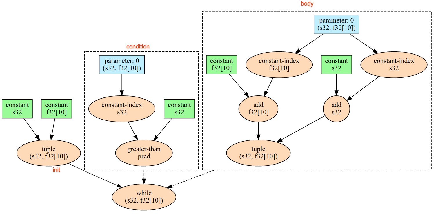
현재
XlaBuilder::While도 참고하세요.
While(condition, body, init)
| 인수 | 유형 | 시맨틱 |
|---|---|---|
condition |
XlaComputation |
루프의 종료 조건을 정의하는 T -> PRED 유형의 XlaComputation. |
body |
XlaComputation |
루프 본문을 정의하는 T -> T 유형의 XlaComputation. |
init |
T |
condition 및 body 매개변수의 초기 값입니다. |
condition가 실패할 때까지 순차적으로 body를 실행합니다. 이는 아래에 나열된 차이점과 제한사항을 제외하고 다른 여러 언어의 일반적인 while 루프와 유사합니다.
While노드는body의 마지막 실행 결과인T유형의 값을 반환합니다.T유형의 모양은 정적으로 결정되며 모든 반복에서 동일해야 합니다.
계산의 T 매개변수는 첫 번째 반복에서 init 값으로 초기화되고 이후의 각 반복에서 body의 새 결과로 자동 업데이트됩니다.
While 노드의 주요 사용 사례 중 하나는 신경망에서 반복되는 학습 실행을 구현하는 것입니다. 아래에는 계산을 나타내는 그래프와 함께 단순화된 의사코드가 표시되어 있습니다. 코드는 while_test.cc에서 찾을 수 있습니다.
이 예에서 T 유형은 반복 횟수의 int32와 누산기의 vector[10]로 구성된 Tuple입니다. 1, 000회 반복의 경우 루프는 누산기에 상수 벡터를 계속 추가합니다.
// Pseudocode for the computation.
init = {0, zero_vector[10]} // Tuple of int32 and float[10].
result = init;
while (result(0) < 1000) {
  iteration = result(0) + 1;
  new_vector = result(1) + constant_vector[10];
  result = {iteration, new_vector};
}