Ниже описывается семантика операций, определенных в интерфейсе XlaBuilder . Обычно эти операции однозначно сопоставляются с операциями, определенными в интерфейсе RPC в xla_data.proto .
Примечание по номенклатуре: обобщенный тип данных, с которым работает XLA, представляет собой N-мерный массив, содержащий элементы некоторого универсального типа (например, 32-битное число с плавающей запятой). В документации массив используется для обозначения массива произвольной размерности. Для удобства особые случаи имеют более конкретные и привычные названия; например, вектор — это одномерный массив, а матрица — двумерный массив.
После всего
См. также XlaBuilder::AfterAll .
AfterAll принимает переменное количество токенов и создает один токен. Токены — это примитивные типы, которые можно объединять между побочными операциями для обеспечения порядка. AfterAll можно использовать как объединение токенов для упорядочивания операции после набора операций.
AfterAll(operands)
| Аргументы | Тип | Семантика |
|---|---|---|
operands | XlaOp | вариативное число токенов |
Всесобрать
См. также XlaBuilder::AllGather .
Выполняет объединение реплик.
AllGather(operand, all_gather_dim, shard_count, replica_group_ids, channel_id)
| Аргументы | Тип | Семантика |
|---|---|---|
operand | XlaOp | Массив для объединения реплик |
all_gather_dim | int64 | Измерение конкатенации |
replica_groups | вектор векторов int64 | Группы, между которыми производится конкатенация |
channel_id | необязательный int64 | Дополнительный идентификатор канала для межмодульной связи |
-
replica_groups— список групп реплик, между которыми выполняется конкатенация (идентификатор реплики для текущей реплики можно получить с помощьюReplicaId). Порядок реплик в каждой группе определяет порядок, в котором их входы располагаются в результате.replica_groupsдолжны быть либо пустыми (в этом случае все реплики принадлежат одной группе, упорядоченной от0доN - 1), либо содержать то же количество элементов, что и количество реплик. Например,replica_groups = {0, 2}, {1, 3}выполняет конкатенацию между репликами0и2, а также1и3. -
shard_count— размер каждой группы реплик. Нам это нужно в тех случаях, когдаreplica_groupsпусты. -
channel_idиспользуется для межмодульной связи: только операцииall-gatherс одинаковымchannel_idмогут взаимодействовать друг с другом.
Выходная форма — это входная форма, в которой all_gather_dim увеличен в разы shard_count . Например, если есть две реплики и операнд имеет значение [1.0, 2.5] и [3.0, 5.25] соответственно для двух реплик, то выходное значение этой операции, где all_gather_dim равно 0 , будет [1.0, 2.5, 3.0, 5.25] на обеих репликах.
AllReduce
См. также XlaBuilder::AllReduce .
Выполняет пользовательские вычисления между репликами.
AllReduce(operand, computation, replica_group_ids, channel_id)
| Аргументы | Тип | Семантика |
|---|---|---|
operand | XlaOp | Массив или непустой кортеж массивов для сокращения количества реплик. |
computation | XlaComputation | Вычисление сокращения |
replica_groups | вектор векторов int64 | Группы, между которыми выполняются сокращения |
channel_id | необязательный int64 | Дополнительный идентификатор канала для межмодульной связи |
- Если
operandпредставляет собой кортеж массивов, полное сокращение выполняется для каждого элемента кортежа. -
replica_groups— список групп реплик, между которыми выполняется сокращение (идентификатор реплики для текущей реплики можно получить с помощьюReplicaId).replica_groupsдолжны быть либо пустыми (в этом случае все реплики принадлежат одной группе), либо содержать то же количество элементов, что и количество реплик. Например,replica_groups = {0, 2}, {1, 3}выполняет сокращение между репликами0и2, а также1и3. -
channel_idиспользуется для межмодульной связи: только операцииall-reduceс одинаковымchannel_idмогут взаимодействовать друг с другом.
Выходная форма такая же, как и входная. Например, если есть две реплики и операнд имеет значение [1.0, 2.5] и [3.0, 5.25] соответственно на двух репликах, то выходное значение этой операции и вычисления суммирования будет [4.0, 7.75] на обеих репликах. реплики. Если входные данные представляют собой кортеж, выходные данные также являются кортежами.
Для вычисления результата AllReduce требуется один вход от каждой реплики, поэтому, если одна реплика выполняет узел AllReduce больше раз, чем другая, то бывшая реплика будет ждать вечно. Поскольку все реплики выполняют одну и ту же программу, это может произойти не так уж и много способов, но это возможно, когда состояние цикла while зависит от данных из ввода, а поступающие данные заставляют цикл while повторяться больше раз. на одной реплике, чем на другой.
ВсеВсеВсе
См. также XlaBuilder::AllToAll .
AllToAll — это коллективная операция, которая отправляет данные со всех ядер на все ядра. Он имеет две фазы:
- Фаза разброса. На каждом ядре операнд разбивается на число блоков
split_countпоsplit_dimensions, и блоки распределяются по всем ядрам, например, i-й блок отправляется на i-е ядро. - Фаза сбора. Каждое ядро объединяет полученные блоки по
concat_dimension.
Участвующие ядра можно настроить следующим образом:
-
replica_groups: каждая ReplicaGroup содержит список идентификаторов реплик, участвующих в вычислении (идентификатор реплики для текущей реплики можно получить с помощьюReplicaId). AllToAll будет применяться внутри подгрупп в указанном порядке. Например,replica_groups = { {1,2,3}, {4,5,0} }означает, что AllToAll будет применяться внутри реплик{1, 2, 3}и на этапе сбора, а полученные блоки будут быть объединены в том же порядке: 1, 2, 3. Затем в репликах 4, 5, 0 будет применен еще один AllToAll, а порядок объединения также равен 4, 5, 0. Если вreplica_groupsпусто, все реплики принадлежат одной группы в порядке их появления.
Предпосылки:
- Размер измерения операнда в
split_dimensionделится наsplit_count. - Форма операнда не является кортежем.
AllToAll(operand, split_dimension, concat_dimension, split_count, replica_groups)
| Аргументы | Тип | Семантика |
|---|---|---|
operand | XlaOp | n-мерный входной массив |
split_dimension | int64 | Значение в интервале [0, n) , обозначающее измерение, по которому разбивается операнд. |
concat_dimension | int64 | Значение в интервале [0, n) , обозначающее измерение, по которому объединяются разделенные блоки. |
split_count | int64 | Количество ядер, участвующих в этой операции. Если replica_groups пуст, это должно быть количество реплик; в противном случае оно должно быть равно количеству реплик в каждой группе. |
replica_groups | Вектор ReplicaGroup | Каждая группа содержит список идентификаторов реплик. |
Ниже показан пример Alltoall.
XlaBuilder b("alltoall");
auto x = Parameter(&b, 0, ShapeUtil::MakeShape(F32, {4, 16}), "x");
AllToAll(x, /*split_dimension=*/1, /*concat_dimension=*/0, /*split_count=*/4);
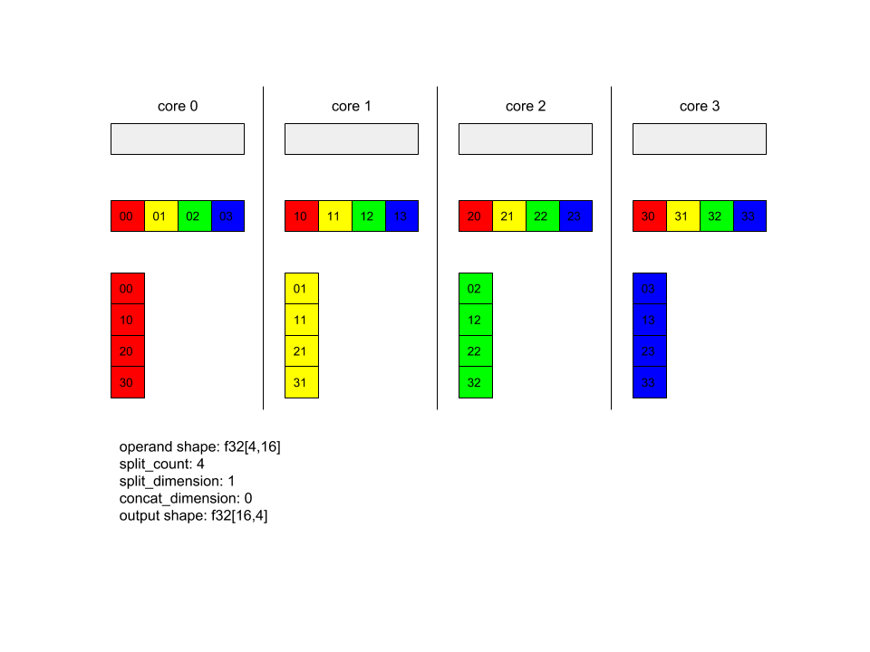
В этом примере в Alltoall участвуют 4 ядра. В каждом ядре операнд разбивается на 4 части по размерности 0, поэтому каждая часть имеет форму f32[4,4]. 4 части разбросаны по всем ядрам. Затем каждое ядро объединяет полученные части по размерности 1 в порядке ядра 0-4. Таким образом, выходные данные каждого ядра имеют форму f32[16,4].
ПакетныйНормаГрад
См. также XlaBuilder::BatchNormGrad и исходный документ по пакетной нормализации для подробного описания алгоритма.
Рассчитывает градиенты нормы партии.
BatchNormGrad(operand, scale, mean, variance, grad_output, epsilon, feature_index)
| Аргументы | Тип | Семантика |
|---|---|---|
operand | XlaOp | n-мерный массив, который нужно нормализовать (x) |
scale | XlaOp | 1-мерный массив (\(\gamma\)) |
mean | XlaOp | 1-мерный массив (\(\mu\)) |
variance | XlaOp | 1-мерный массив (\(\sigma^2\)) |
grad_output | XlaOp | Градиенты, передаваемые в BatchNormTraining (\(\nabla y\)) |
epsilon | float | Значение Эпсилон (\(\epsilon\)) |
feature_index | int64 | Индекс для измерения функции в operand |
Для каждого объекта в измерении объекта ( feature_index — это индекс измерения объекта в operand ) операция вычисляет градиенты относительно operand , offset и scale по всем остальным измерениям. feature_index должен быть допустимым индексом для измерения объекта в operand .
Три градиента определяются следующими формулами (предполагая, что 4-мерный массив является operand и имеет индекс измерения объекта l , размер пакета m и пространственные размеры w и h ):
\[ \begin{split} c_l&= \frac{1}{mwh}\sum_{i=1}^m\sum_{j=1}^w\sum_{k=1}^h \left( \nabla y_{ijkl} \frac{x_{ijkl} - \mu_l}{\sigma^2_l+\epsilon} \right) \\\\ d_l&= \frac{1}{mwh}\sum_{i=1}^m\sum_{j=1}^w\sum_{k=1}^h \nabla y_{ijkl} \\\\ \nabla x_{ijkl} &= \frac{\gamma_{l} }{\sqrt{\sigma^2_{l}+\epsilon} } \left( \nabla y_{ijkl} - d_l - c_l (x_{ijkl} - \mu_{l}) \right) \\\\ \nabla \gamma_l &= \sum_{i=1}^m\sum_{j=1}^w\sum_{k=1}^h \left( \nabla y_{ijkl} \frac{x_{ijkl} - \mu_l}{\sqrt{\sigma^2_{l}+\epsilon} } \right) \\\\\ \nabla \beta_l &= \sum_{i=1}^m\sum_{j=1}^w\sum_{k=1}^h \nabla y_{ijkl} \end{split} \]
Входные данные mean и variance представляют значения моментов по партиям и пространственным измерениям.
Тип вывода представляет собой кортеж из трех дескрипторов:
| Выходы | Тип | Семантика |
|---|---|---|
grad_operand | XlaOp | градиент относительно входного operand ($\nabla x$) |
grad_scale | XlaOp | градиент относительно входного scale ($\nabla \gamma$) |
grad_offset | XlaOp | градиент относительно входного offset ($\nabla \beta$) |
Пакетная нормаВывод
См. также XlaBuilder::BatchNormInference и исходный документ по пакетной нормализации для подробного описания алгоритма.
Нормализует массив по пакетным и пространственным измерениям.
BatchNormInference(operand, scale, offset, mean, variance, epsilon, feature_index)
| Аргументы | Тип | Семантика |
|---|---|---|
operand | XlaOp | n-мерный массив, который нужно нормализовать |
scale | XlaOp | 1-мерный массив |
offset | XlaOp | 1-мерный массив |
mean | XlaOp | 1-мерный массив |
variance | XlaOp | 1-мерный массив |
epsilon | float | Значение Эпсилон |
feature_index | int64 | Индекс для измерения функции в operand |
Для каждого объекта в измерении объекта ( feature_index — это индекс измерения объекта в operand ) операция вычисляет среднее значение и дисперсию по всем остальным измерениям и использует среднее значение и дисперсию для нормализации каждого элемента в operand . feature_index должен быть допустимым индексом для измерения объекта в operand .
BatchNormInference эквивалентен вызову BatchNormTraining без вычисления mean и variance для каждой партии. Вместо этого в качестве оценочных значений используются входное mean и variance . Цель этой операции — уменьшить задержку вывода, отсюда и название BatchNormInference .
Выходные данные представляют собой n-мерный нормализованный массив той же формы, что и входной operand .
Пакетная нормаОбучение
См. также XlaBuilder::BatchNormTraining и the original batch normalization paper для подробного описания алгоритма.
Нормализует массив по пакетным и пространственным измерениям.
BatchNormTraining(operand, scale, offset, epsilon, feature_index)
| Аргументы | Тип | Семантика |
|---|---|---|
operand | XlaOp | n-мерный массив, который нужно нормализовать (x) |
scale | XlaOp | 1-мерный массив (\(\gamma\)) |
offset | XlaOp | 1-мерный массив (\(\beta\)) |
epsilon | float | Значение Эпсилон (\(\epsilon\)) |
feature_index | int64 | Индекс для измерения функции в operand |
Для каждого объекта в измерении объекта ( feature_index — это индекс измерения объекта в operand ) операция вычисляет среднее значение и дисперсию по всем остальным измерениям и использует среднее значение и дисперсию для нормализации каждого элемента в operand . feature_index должен быть допустимым индексом для измерения объекта в operand .
Алгоритм работает следующим образом для каждого пакета в operand \(x\) , который содержит m элементов с w и h в качестве размера пространственного измерения (при условии, что operand представляет собой 4-мерный массив):
Вычисляет среднее значение партии \(\mu_l\) для каждого объекта
lв измерении объекта:\(\mu_l=\frac{1}{mwh}\sum_{i=1}^m\sum_{j=1}^w\sum_{k=1}^h x_{ijkl}\)Вычисляет дисперсию партии \(\sigma^2_l\): $\sigma^2 l=\frac{1}{mwh}\sum {i=1}^m\sum {j=1}^w\sum {k=1}^h ( x_{ijkl} - \mu_l)^2$
Нормализует, масштабирует и сдвигает:\(y_{ijkl}=\frac{\gamma_l(x_{ijkl}-\mu_l)}{\sqrt[2]{\sigma^2_l+\epsilon} }+\beta_l\)
Значение эпсилон, обычно небольшое число, добавляется во избежание ошибок деления на ноль.
Тип вывода — это кортеж из трех XlaOp :
| Выходы | Тип | Семантика |
|---|---|---|
output | XlaOp | n-мерный массив той же формы, что и входной operand (y) |
batch_mean | XlaOp | 1-мерный массив (\(\mu\)) |
batch_var | XlaOp | 1-мерный массив (\(\sigma^2\)) |
batch_mean и batch_var — это моменты, рассчитанные для партии и пространственных измерений с использованием приведенных выше формул.
BitcastConvertType
См. также XlaBuilder::BitcastConvertType .
Подобно tf.bitcast в TensorFlow, выполняет поэлементную операцию преобразования битов из формы данных в целевую форму. Размер ввода и вывода должен совпадать: например, элементы s32 становятся элементами f32 посредством процедуры битового вещания, а один элемент s32 станет четырьмя элементами s8 . Bitcast реализован как низкоуровневое приведение, поэтому машины с разными представлениями чисел с плавающей запятой будут давать разные результаты.
BitcastConvertType(operand, new_element_type)
| Аргументы | Тип | Семантика |
|---|---|---|
operand | XlaOp | массив типа T с размерами D |
new_element_type | PrimitiveType | тип U |
Размеры операнда и целевой формы должны совпадать, за исключением последнего измерения, которое изменится на соотношение размера примитива до и после преобразования.
Типы элементов источника и назначения не должны быть кортежами.
Bitcast-преобразование в примитивный тип разной ширины
Инструкция BitcastConvert HLO поддерживает случай, когда размер выходного элемента типа T' не равен размеру входного элемента T . Поскольку вся операция концептуально является битовой передачей и не меняет базовые байты, форма выходного элемента должна измениться. Для B = sizeof(T), B' = sizeof(T') возможны два случая.
Во-первых, когда B > B' , выходная форма получает новое наименьшее измерение размера B/B' . Например:
f16[10,2]{1,0} %output = f16[10,2]{1,0} bitcast-convert(f32[10]{0} %input)
Для эффективных скаляров правило остается тем же:
f16[2]{0} %output = f16[2]{0} bitcast-convert(f32[] %input)
Альтернативно, для B' > B инструкция требует, чтобы последний логический размер входной формы был равен B'/B , и этот размер удаляется во время преобразования:
f32[10]{0} %output = f32[10]{0} bitcast-convert(f16[10,2]{1,0} %input)
Обратите внимание, что преобразования между различными разрядностями не выполняются поэлементно.
Транслировать
См. также XlaBuilder::Broadcast .
Добавляет измерения в массив путем дублирования данных в массиве.
Broadcast(operand, broadcast_sizes)
| Аргументы | Тип | Семантика |
|---|---|---|
operand | XlaOp | Массив для дублирования |
broadcast_sizes | ArraySlice<int64> | Размеры новых габаритов |
Новые измерения вставляются слева, т.е. если broadcast_sizes имеет значения {a0, ..., aN} , а форма операнда имеет размеры {b0, ..., bM} , то форма вывода имеет размеры {a0, ..., aN, b0, ..., bM} .
Новый размерный индекс копий операнда, т.е.
output[i0, ..., iN, j0, ..., jM] = operand[j0, ..., jM]
Например, если operand — скаляр f32 со значением 2.0f , а broadcast_sizes — {2, 3} , то результатом будет массив формы f32[2, 3] и все значения в результате будут равны 2.0f .
BroadcastInDim
См. также XlaBuilder::BroadcastInDim .
Увеличивает размер и ранг массива путем дублирования данных в массиве.
BroadcastInDim(operand, out_dim_size, broadcast_dimensions)
| Аргументы | Тип | Семантика |
|---|---|---|
operand | XlaOp | Массив для дублирования |
out_dim_size | ArraySlice<int64> | Размеры габаритов целевой формы |
broadcast_dimensions | ArraySlice<int64> | Какому измерению целевой формы соответствует каждое измерение формы операнда? |
Похож на Broadcast, но позволяет добавлять измерения где угодно и расширять существующие измерения размером 1.
operand транслируется в форму, описанную out_dim_size . broadcast_dimensions сопоставляет размеры operand с размерами целевой фигуры, т. е. i-е измерение операнда сопоставляется с Broadcast_dimension[i]-м измерением выходной формы. Размеры operand должны иметь размер 1 или тот же размер, что и размер выходной фигуры, с которой они сопоставляются. Остальные измерения заполняются измерениями размера 1. Затем вещание вырожденного измерения транслируется по этим вырожденным измерениям для достижения выходной формы. Семантика подробно описана на странице трансляции .
Вызов
См. также XlaBuilder::Call .
Вызывает вычисление с заданными аргументами.
Call(computation, args...)
| Аргументы | Тип | Семантика |
|---|---|---|
computation | XlaComputation | вычисление типа T_0, T_1, ..., T_{N-1} -> S с N параметрами произвольного типа |
args | последовательность N XlaOp | N аргументов произвольного типа |
Арность и типы args должны соответствовать параметрам computation . Допускается отсутствие args .
Холеский
См. также XlaBuilder::Cholesky .
Вычисляет разложение Холецкого группы симметричных (эрмитовых) положительно определенных матриц.
Cholesky(a, lower)
| Аргументы | Тип | Семантика |
|---|---|---|
a | XlaOp | массив ранга > 2 комплексного типа или типа с плавающей запятой. |
lower | bool | использовать ли верхний или нижний a . |
Если lower имеет значение true , вычисляет нижние треугольные матрицы l такие, что $a = l . л^Т$. Если lower имеет значение false , вычисляет верхнетреугольные матрицы u такие, что\(a = u^T . u\).
Входные данные считываются только из нижнего/верхнего треугольника a , в зависимости от значения lower . Значения из другого треугольника игнорируются. Выходные данные возвращаются в том же треугольнике; значения в другом треугольнике определяются реализацией и могут быть любыми.
Если ранг a больше 2, a рассматривается как пакет матриц, где все измерения, за исключением младших двух, являются измерениями пакета.
Если a не является симметричным (эрмитовым) положительно определенным, результат определяется реализацией.
Зажим
См. также XlaBuilder::Clamp .
Фиксирует операнд в пределах диапазона между минимальным и максимальным значением.
Clamp(min, operand, max)
| Аргументы | Тип | Семантика |
|---|---|---|
min | XlaOp | массив типа Т |
operand | XlaOp | массив типа Т |
max | XlaOp | массив типа Т |
Учитывая операнд и минимальное и максимальное значения, возвращает операнд, если он находится в диапазоне между минимальным и максимальным, иначе возвращает минимальное значение, если операнд находится ниже этого диапазона, или максимальное значение, если операнд находится выше этого диапазона. То есть clamp(a, x, b) = min(max(a, x), b) .
Все три массива должны быть одинаковой формы. В качестве альтернативы, в качестве ограниченной формы широковещания , min и/или max могут быть скаляром типа T
Пример со скалярными min и max :
let operand: s32[3] = {-1, 5, 9};
let min: s32 = 0;
let max: s32 = 6;
==>
Clamp(min, operand, max) = s32[3]{0, 5, 6};
Крах
См. также XlaBuilder::Collapse и операцию tf.reshape .
Сворачивает размеры массива в одно измерение.
Collapse(operand, dimensions)
| Аргументы | Тип | Семантика |
|---|---|---|
operand | XlaOp | массив типа Т |
dimensions | вектор int64 | упорядоченное, последовательное подмножество измерений T. |
Свернуть заменяет заданное подмножество измерений операнда одним измерением. Входные аргументы представляют собой произвольный массив типа T и вектор индексов размерностей, постоянный во время компиляции. Индексы измерений должны представлять собой упорядоченное (от низкого до высокого числа измерений) последовательное подмножество измерений T. Таким образом, {0, 1, 2}, {0, 1} или {1, 2} являются допустимыми наборами измерений, а {1, 0} или {0, 2} — нет. Они заменяются одним новым размером, находящимся в той же позиции в последовательности размеров, что и те, которые они заменяют, с новым размером размера, равным произведению размеров исходного размера. Наименьшее число измерений в dimensions — это самое медленно меняющееся измерение (наиболее важное) в гнезде циклов, которое схлопывает эти измерения, а наибольшее число измерений — это самое быстро меняющееся (наиболее незначительное). См. оператор tf.reshape , если требуется более общий порядок свертывания.
Например, пусть v — массив из 24 элементов:
let v = f32[4x2x3] { { {10, 11, 12},  {15, 16, 17} },
{ {20, 21, 22},  {25, 26, 27} },
{ {30, 31, 32},  {35, 36, 37} },
{ {40, 41, 42},  {45, 46, 47} } };

// Collapse to a single dimension, leaving one dimension.
let v012 = Collapse(v, {0,1,2});
then v012 == f32[24] {10, 11, 12, 15, 16, 17,
20, 21, 22, 25, 26, 27,
30, 31, 32, 35, 36, 37,
40, 41, 42, 45, 46, 47};

// Collapse the two lower dimensions, leaving two dimensions.
let v01 = Collapse(v, {0,1});
then v01 == f32[4x6] { {10, 11, 12, 15, 16, 17},
{20, 21, 22, 25, 26, 27},
{30, 31, 32, 35, 36, 37},
{40, 41, 42, 45, 46, 47} };

// Collapse the two higher dimensions, leaving two dimensions.
let v12 = Collapse(v, {1,2});
then v12 == f32[8x3] { {10, 11, 12},
{15, 16, 17},
{20, 21, 22},
{25, 26, 27},
{30, 31, 32},
{35, 36, 37},
{40, 41, 42},
{45, 46, 47} };
КоллективныйPermute
См. также XlaBuilder::CollectivePermute .
CollectivePermute — это коллективная операция, которая отправляет и получает перекрестные реплики данных.
CollectivePermute(operand, source_target_pairs)
| Аргументы | Тип | Семантика |
|---|---|---|
operand | XlaOp | n-мерный входной массив |
source_target_pairs | вектор <int64, int64> | Список пар (source_replica_id, target_replica_id). Для каждой пары операнд отправляется из исходной реплики в целевую реплику. |
Обратите внимание, что на source_target_pair существуют следующие ограничения:
- Любые две пары не должны иметь одинаковый идентификатор целевой реплики и не должны иметь одинаковый идентификатор исходной реплики.
- Если идентификатор реплики не является целью ни в одной паре, то выходные данные этой реплики представляют собой тензор, состоящий из 0(ов) той же формы, что и входные данные.
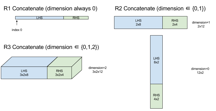
Объединить
См. также XlaBuilder::ConcatInDim .
Конкатенация составляет массив из нескольких операндов массива. Массив имеет тот же ранг, что и каждый из операндов входного массива (которые должны быть того же ранга, что и другие), и содержит аргументы в том порядке, в котором они были указаны.
Concatenate(operands..., dimension)
| Аргументы | Тип | Семантика |
|---|---|---|
operands | последовательность N XlaOp | N массивов типа T размерностей [L0, L1, ...]. Требуется N >= 1. |
dimension | int64 | Значение в интервале [0, N) , определяющее измерение, которое необходимо объединить между operands . |
За исключением dimension все размеры должны быть одинаковыми. Это связано с тем, что XLA не поддерживает «рваные» массивы. Также обратите внимание, что значения ранга 0 не могут быть объединены (поскольку невозможно указать измерение, по которому происходит объединение).
1-мерный пример:
Concat({ {2, 3}, {4, 5}, {6, 7} }, 0)
>>> {2, 3, 4, 5, 6, 7}
2-мерный пример:
let a = {
{1, 2},
{3, 4},
{5, 6},
};
let b = {
{7, 8},
};
Concat({a, b}, 0)
>>> {
{1, 2},
{3, 4},
{5, 6},
{7, 8},
}
Диаграмма:
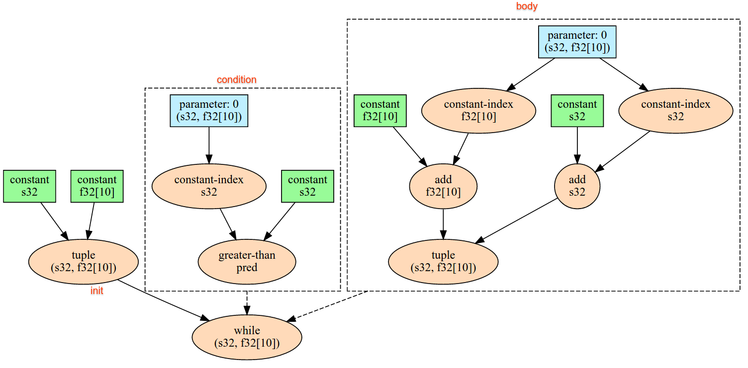
Условный
См. также XlaBuilder::Conditional .
Conditional(pred, true_operand, true_computation, false_operand, false_computation)
| Аргументы | Тип | Семантика |
|---|---|---|
pred | XlaOp | Скаляр типа PRED |
true_operand | XlaOp | Аргумент типа \(T_0\) |
true_computation | XlaComputation | XlaВычисление типа \(T_0 \to S\) |
false_operand | XlaOp | Аргумент типа \(T_1\) |
false_computation | XlaComputation | XlaВычисление типа \(T_1 \to S\) |
Выполняет true_computation если pred имеет true , false_computation если pred имеет значение false , и возвращает результат.
true_computation должен принимать один аргумент типа \(T_0\) и будет вызываться с true_operand , который должен быть того же типа. false_computation принимать один аргумент типа \(T_1\) и будет вызываться с false_operand , который должен быть того же типа. Тип возвращаемого значения true_computation и false_computation должен быть одинаковым.
Обратите внимание, что в зависимости от значения pred будет выполнено только одно из true_computation и false_computation .
Conditional(branch_index, branch_computations, branch_operands)
| Аргументы | Тип | Семантика |
|---|---|---|
branch_index | XlaOp | Скаляр типа S32 |
branch_computations | последовательность N XlaComputation | XlaВычисления типа \(T_0 \to S , T_1 \to S , ..., T_{N-1} \to S\) |
branch_operands | последовательность N XlaOp | Аргументы типа \(T_0 , T_1 , ..., T_{N-1}\) |
Выполняет branch_computations[branch_index] и возвращает результат. Если branch_index — это S32 , который равен < 0 или >= N, то branch_computations[N-1] выполняется как ветвь по умолчанию.
Каждая branch_computations[b] должна принимать один аргумент типа \(T_b\) и будет вызываться с помощью branch_operands[b] , которая должна быть того же типа. Тип возвращаемого значения каждого branch_computations[b] должен быть одинаковым.
Обратите внимание, что только одно из branch_computations будет выполнено в зависимости от значения branch_index .
Конв (свертка)
См. также XlaBuilder::Conv .
Как и ConvWithGeneralPadding, но заполнение указывается сокращенно: SAME или VALID. SAME дополнение дополняет входные данные ( lhs ) нулями, чтобы выходные данные имели ту же форму, что и входные, если не принимать во внимание шаг. ДЕЙСТВИТЕЛЬНОЕ дополнение просто означает отсутствие заполнения.
ConvWithGeneralPadding (свертка)
См. также XlaBuilder::ConvWithGeneralPadding .
Вычисляет свертку, используемую в нейронных сетях. Здесь свертку можно рассматривать как n-мерное окно, перемещающееся по n-мерной базовой области, и вычисления выполняются для каждой возможной позиции окна.
| Аргументы | Тип | Семантика |
|---|---|---|
lhs | XlaOp | ранг n+2 массива входов |
rhs | XlaOp | ранг n+2 массива весов ядра |
window_strides | ArraySlice<int64> | й массив шагов ядра |
padding | ArraySlice< pair<int64,int64>> | nd массив (низкий, высокий) заполнения |
lhs_dilation | ArraySlice<int64> | Массив коэффициентов расширения nd lhs |
rhs_dilation | ArraySlice<int64> | Массив коэффициентов расширения nd rhs |
feature_group_count | int64 | количество групп функций |
batch_group_count | int64 | количество пакетных групп |
Пусть n — количество пространственных измерений. Аргумент lhs представляет собой массив ранга n+2, описывающий базовую область. Это называется входом, хотя, конечно, правая часть тоже является входом. В нейронной сети это входные активации. Размеры n+2 в следующем порядке:
-
batch: каждая координата в этом измерении представляет собой независимый вход, для которого выполняется свертка. -
z/depth/features: каждая позиция (y,x) в базовой области имеет связанный с ней вектор, который входит в это измерение. -
spatial_dims: описываетnпространственных измерений, определяющих базовую область, по которой перемещается окно.
Аргумент rhs представляет собой массив ранга n+2, описывающий сверточный фильтр/ядро/окно. Размеры в таком порядке:
-
output-z: размер выходных данных по осиz -
input-z: размер этого измерения, умноженныйfeature_group_countдолжен равняться размеру измеренияzв левой стороне. -
spatial_dims: описываетnпространственных измерений, которые определяют окно, перемещающееся по базовой области.
Аргумент window_strides определяет шаг сверточного окна в пространственных измерениях. Например, если шаг в первом пространственном измерении равен 3, то окно можно разместить только в координатах, где первый пространственный индекс делится на 3.
Аргумент padding указывает величину заполнения нулями, которая будет применена к базовой области. Величина заполнения может быть отрицательной — абсолютное значение отрицательного заполнения указывает количество элементов, которые необходимо удалить из указанного измерения перед выполнением свертки. padding[0] задает заполнение для измерения y , а padding[1] задает заполнение для измерения x . Каждая пара имеет нижнее дополнение в качестве первого элемента и высокое дополнение в качестве второго элемента. Низкое заполнение применяется в направлении более низких индексов, тогда как высокое заполнение применяется в направлении более высоких индексов. Например, если padding[1] равно (2,3) то во втором пространственном измерении будет дополнение на 2 нуля слева и на 3 нуля справа. Использование заполнения эквивалентно вставке тех же нулевых значений во входные данные ( lhs ) перед выполнением свертки.
Аргументы lhs_dilation и rhs_dilation определяют коэффициент расширения, который будет применяться к левой и правой границам соответственно в каждом пространственном измерении. Если коэффициент расширения в пространственном измерении равен d, то между каждым элементом этого измерения неявно размещаются отверстия d-1, увеличивая размер массива. Дыры заполняются пустым значением, которое для свертки означает нули.
Дилатацию резцов также называют атрозной извилиной. Более подробную информацию см. в tf.nn.atrous_conv2d . Расширение левой стороны также называется транспонированной сверткой. Более подробную информацию см. в tf.nn.conv2d_transpose .
Аргумент feature_group_count (значение по умолчанию 1) можно использовать для сгруппированных сверток. feature_group_count должен быть делителем как входного, так и выходного измерения объекта. Если feature_group_count больше 1, это означает, что концептуально измерение входного и выходного объекта, а также измерение выходного объекта rhs равномерно разделены на множество групп feature_group_count , каждая группа состоит из последовательной подпоследовательности объектов. Размер входного объекта rhs должен быть равен размеру входного объекта lhs , разделенному на feature_group_count (так что он уже имеет размер группы входных объектов). i-ые группы используются вместе для вычисления feature_group_count для множества отдельных сверток. Результаты этих сверток объединяются в измерении выходного объекта.
Для глубинной свертки аргумент feature_group_count будет установлен в размер входного объекта, а форма фильтра будет изменена с [filter_height, filter_width, in_channels, channel_multiplier] на [filter_height, filter_width, 1, in_channels * channel_multiplier] . Более подробную информацию см. в tf.nn.depthwise_conv2d .
Аргумент batch_group_count (значение по умолчанию 1) можно использовать для сгруппированных фильтров во время обратного распространения ошибки. batch_group_count должен быть делителем размера lhs (входного) измерения пакета. Если batch_group_count больше 1, это означает, что размерность выходного пакета должна иметь размер input batch / batch_group_count . batch_group_count должен быть делителем размера выходного объекта.
Выходная форма имеет следующие размеры в следующем порядке:
-
batch: размер этого измерения, умноженныйbatch_group_count, должен равняться размеру измеренияbatchв левых единицах измерения. -
z: тот же размер, что и уoutput-zв ядре (rhs). -
spatial_dims: одно значение для каждого допустимого размещения сверточного окна.

На рисунке выше показано, как работает поле batch_group_count . По сути, мы делим каждый пакет lhs на группы batch_group_count и делаем то же самое для выходных объектов. Затем для каждой из этих групп мы выполняем попарные свертки и объединяем выходные данные по измерению выходного объекта. Операционная семантика всех других измерений (особенностей и пространственного) остается прежней.
Допустимое размещение сверточного окна определяется шагами и размером базовой области после заполнения.
Чтобы описать, что делает свертка, рассмотрим двумерную свертку и выберите на выходе некоторую фиксированную batch координат z , y , x . Тогда (y,x) — это положение угла окна в базовой области (например, верхний левый угол, в зависимости от того, как вы интерпретируете пространственные измерения). Теперь у нас есть 2D-окно, взятое из базовой области, где каждая 2D-точка связана с 1D-вектором, поэтому мы получаем 3D-окно. Из сверточного ядра, поскольку мы зафиксировали выходную координату z , у нас также есть 3D-бокс. Два блока имеют одинаковые размеры, поэтому мы можем взять сумму поэлементных произведений между двумя блоками (аналогично скалярному произведению). Это выходное значение.
Обратите внимание, что если output-z равно, например, 5, то каждая позиция окна создает 5 значений на выходе в измерении z вывода. Эти значения различаются тем, какая часть сверточного ядра используется — для каждой координаты output-z используется отдельный трехмерный блок значений. Таким образом, вы можете думать об этом как о 5 отдельных свертках с разными фильтрами для каждой из них.
Вот псевдокод для 2d-свертки с заполнением и шагом:
for (b, oz, oy, ox) {  // output coordinates
  value = 0;
  for (iz, ky, kx) {  // kernel coordinates and input z
    iy = oy*stride_y + ky - pad_low_y;
    ix = ox*stride_x + kx - pad_low_x;
    if ((iy, ix) inside the base area considered without padding) {
      value += input(b, iz, iy, ix) * kernel(oz, iz, ky, kx);
    }
  }
  output(b, oz, oy, ox) = value;
}
КонвертироватьЭлементТип
См. также XlaBuilder::ConvertElementType .
Подобно поэлементному static_cast в C++, выполняет поэлементную операцию преобразования из формы данных в целевую фигуру. Размеры должны совпадать, а преобразование — поэлементное; например, элементы s32 становятся элементами f32 посредством процедуры преобразования s32 в f32 .
ConvertElementType(operand, new_element_type)
| Аргументы | Тип | Семантика |
|---|---|---|
operand | XlaOp | массив типа T с размерами D |
new_element_type | PrimitiveType | тип U |
Размеры операнда и целевой формы должны совпадать. Типы элементов источника и назначения не должны быть кортежами.
Преобразование, такое как T=s32 в U=f32 , выполнит процедуру нормализации преобразования целого числа в число с плавающей запятой, например округление до ближайшего четного.
let a: s32[3] = {0, 1, 2};
let b: f32[3] = convert(a, f32);
then b == f32[3]{0.0, 1.0, 2.0}
CrossReplicaSum
Выполняет AllReduce с вычислением суммирования.
Пользовательский вызов
См. также XlaBuilder::CustomCall .
Вызов предоставленной пользователем функции в рамках вычисления.
CustomCall(target_name, args..., shape)
| Аргументы | Тип | Семантика |
|---|---|---|
target_name | string | Имя функции. Будет выдана инструкция вызова, нацеленная на это имя символа. |
args | последовательность N XlaOp | N аргументов произвольного типа, которые будут переданы в функцию. |
shape | Shape | Выходная форма функции |
Сигнатура функции одинакова, независимо от арности или типа аргументов:
extern "C" void target_name(void* out, void** in);
Например, если CustomCall используется следующим образом:
let x = f32[2] {1,2};
let y = f32[2x3] { {10, 20, 30}, {40, 50, 60} };

CustomCall("myfunc", {x, y}, f32[3x3])
Вот пример реализации myfunc :
extern "C" void myfunc(void* out, void** in) {
  float (&x)[2] = *static_cast<float(*)[2]>(in[0]);
  float (&y)[2][3] = *static_cast<float(*)[2][3]>(in[1]);
  EXPECT_EQ(1, x[0]);
  EXPECT_EQ(2, x[1]);
  EXPECT_EQ(10, y[0][0]);
  EXPECT_EQ(20, y[0][1]);
  EXPECT_EQ(30, y[0][2]);
  EXPECT_EQ(40, y[1][0]);
  EXPECT_EQ(50, y[1][1]);
  EXPECT_EQ(60, y[1][2]);
  float (&z)[3][3] = *static_cast<float(*)[3][3]>(out);
  z[0][0] = x[1] + y[1][0];
  // ...
}
Предоставляемая пользователем функция не должна иметь побочных эффектов, а ее выполнение должно быть идемпотентным.
Точка
См. также XlaBuilder::Dot .
Dot(lhs, rhs)
| Аргументы | Тип | Семантика |
|---|---|---|
lhs | XlaOp | массив типа Т |
rhs | XlaOp | массив типа Т |
Точная семантика этой операции зависит от рангов операндов:
| Вход | Выход | Семантика |
|---|---|---|
вектор [n] dot вектор [n] | скаляр | векторное скалярное произведение |
матрица [mxk] dot вектор [k] | вектор [м] | матрично-векторное умножение |
матрица [mxk] dot матрица [kxn] | матрица [mxn] | умножение матрицы на матрицу |
Операция выполняет суммирование произведений по второму измерению lhs (или первому, если она имеет ранг 1) и первому измерению rhs . Это «сжатые» размеры. Сжатые размеры lhs и rhs должны быть одинакового размера. На практике его можно использовать для скалярного произведения векторов, умножения вектора/матрицы или умножения матрицы/матрицы.
ТочкаОбщий
См. также XlaBuilder::DotGeneral .
DotGeneral(lhs, rhs, dimension_numbers)
| Аргументы | Тип | Семантика |
|---|---|---|
lhs | XlaOp | массив типа Т |
rhs | XlaOp | массив типа Т |
dimension_numbers | DotDimensionNumbers | номера контрактов и размеров партии |
Аналогично Dot, но позволяет указывать номера размеров контрактов и партий как для lhs , так и rhs .
| Поля DotDimensionNumbers | Тип | Семантика |
|---|---|---|
lhs_contracting_dimensions | повторный int64 | цифры контрактных размеров lhs |
rhs_contracting_dimensions | повторный int64 | цифры договорных размеров rhs |
lhs_batch_dimensions | повторный int64 | lhs номера размеров партии |
rhs_batch_dimensions | повторный int64 | номера размеров партии rhs |
DotGeneral выполняет суммирование продуктов по контрактным измерениям, указанным в dimension_numbers .
Соответствующие номера контрактных размеров lhs и rhs не обязательно должны быть одинаковыми, но должны иметь одинаковые размеры.
Пример с номерами сжимающих размеров:
lhs = { {1.0, 2.0, 3.0},
{4.0, 5.0, 6.0} }

rhs = { {1.0, 1.0, 1.0},
{2.0, 2.0, 2.0} }

DotDimensionNumbers dnums;
dnums.add_lhs_contracting_dimensions(1);
dnums.add_rhs_contracting_dimensions(1);

DotGeneral(lhs, rhs, dnums) -> { {6.0, 12.0},
{15.0, 30.0} }
Связанные номера размеров партии из lhs и rhs должны иметь одинаковые размеры.
Пример с номерами размеров партии (размер партии 2, матрицы 2x2):
lhs = { { {1.0, 2.0},
{3.0, 4.0} },
{ {5.0, 6.0},
{7.0, 8.0} } }

rhs = { { {1.0, 0.0},
{0.0, 1.0} },
{ {1.0, 0.0},
{0.0, 1.0} } }

DotDimensionNumbers dnums;
dnums.add_lhs_contracting_dimensions(2);
dnums.add_rhs_contracting_dimensions(1);
dnums.add_lhs_batch_dimensions(0);
dnums.add_rhs_batch_dimensions(0);

DotGeneral(lhs, rhs, dnums) -> { { {1.0, 2.0},
{3.0, 4.0} },
{ {5.0, 6.0},
{7.0, 8.0} } }
| Вход | Выход | Семантика |
|---|---|---|
[b0, m, k] dot [b0, k, n] | [б0, м, н] | пакетный матмул |
[b0, b1, m, k] dot [b0, b1, k, n] | [b0, b1, м, н] | пакетный матмул |
Отсюда следует, что результирующий размерный номер начинается с размера партии, затем lhs несужающегося/непартийного размера и, наконец, с rhs несжимающегося/непартийного размера.
Динамический срез
См. также XlaBuilder::DynamicSlice .
DynamicSlice извлекает подмассив из входного массива в динамическом start_indices . Размер среза в каждом измерении передается в size_indices , который определяет конечную точку эксклюзивных интервалов среза в каждом измерении: [start, start + size). Форма start_indices должна иметь ранг == 1, а размерность равна рангу operand .
DynamicSlice(operand, start_indices, size_indices)
| Аргументы | Тип | Семантика |
|---|---|---|
operand | XlaOp | N-мерный массив типа T |
start_indices | последовательность N XlaOp | Список N скалярных целых чисел, содержащих начальные индексы среза для каждого измерения. Значение должно быть больше или равно нулю. |
size_indices | ArraySlice<int64> | Список из N целых чисел, содержащих размер среза для каждого измерения. Каждое значение должно быть строго больше нуля, а значение start + size должно быть меньше или равно размеру измерения, чтобы избежать переноса по модулю размера измерения. |
Эффективные индексы среза вычисляются путем применения следующего преобразования для каждого индекса i в [1, N) перед выполнением среза:
start_indices[i] = clamp(start_indices[i], 0, operand.dimension_size[i] - size_indices[i])
Это гарантирует, что извлеченный фрагмент всегда находится в пределах массива операндов. Если срез находится в границах до применения преобразования, преобразование не оказывает никакого эффекта.
1-мерный пример:
let a = {0.0, 1.0, 2.0, 3.0, 4.0}
let s = {2}

DynamicSlice(a, s, {2}) produces:
{2.0, 3.0}
2-мерный пример:
let b =
{ {0.0,  1.0,  2.0},
{3.0,  4.0,  5.0},
{6.0,  7.0,  8.0},
{9.0, 10.0, 11.0} }
let s = {2, 1}

DynamicSlice(b, s, {2, 2}) produces:
{ { 7.0,  8.0},
{10.0, 11.0} }
ДинамическийUpdateSlice
См. также XlaBuilder::DynamicUpdateSlice .
Dynamicupdateslice генерирует результат, который является значением operand ввода массива, а update среза перезаписано на start_indices . Форма update определяет форму суб-арайла результата, которая обновляется. Форма start_indices должна быть рангом == 1, с размером измерения, равным рангу operand .
DynamicUpdateSlice(operand, update, start_indices)
| Аргументы | Тип | Семантика |
|---|---|---|
operand | XlaOp | N размерный массив типа T |
update | XlaOp | N размерный массив типа T, содержащий обновление среза. Каждое измерение формы обновления должно быть строго больше нуля, а обновление start + должно быть меньше или равным размеру операнда для каждого измерения, чтобы избежать генерации индексов обновления вне склонов. |
start_indices | последовательность n XlaOp | Список n скалярных целых чисел, содержащих начальные индексы среза для каждого измерения. Значение должно быть больше или равно нулю. |
Эффективные индексы срезов вычисляются путем применения следующего преобразования для каждого индекса i в [1, N) перед выполнением среза:
start_indices[i] = clamp(start_indices[i], 0, operand.dimension_size[i] - update.dimension_size[i])
Это гарантирует, что обновленный ломтик всегда вводится в отношении массива операнда. Если срез вводится до применения преобразования, преобразование не оказывает эффекта.
1-мерный пример:
let a = {0.0, 1.0, 2.0, 3.0, 4.0}
let u = {5.0, 6.0}
let s = {2}

DynamicUpdateSlice(a, u, s) produces:
{0.0, 1.0, 5.0, 6.0, 4.0}
2-мерный пример:
let b =
{ {0.0,  1.0,  2.0},
{3.0,  4.0,  5.0},
{6.0,  7.0,  8.0},
{9.0, 10.0, 11.0} }
let u =
{ {12.0,  13.0},
{14.0,  15.0},
{16.0,  17.0} }

let s = {1, 1}

DynamicUpdateSlice(b, u, s) produces:
{ {0.0,  1.0,  2.0},
{3.0, 12.0, 13.0},
{6.0, 14.0, 15.0},
{9.0, 16.0, 17.0} }
Элементные бинарные арифметические операции
Смотрите также XlaBuilder::Add .
Поддерживается набор бинарных арифметических операций.
Op(lhs, rhs)
Где Op является одним из Add (добавление), Sub (вычитание), Mul (умножение), Div (деление), Rem (остаток), Max (максимум), Min (минимум), LogicalAnd (логический и) или LogicalOr (логический ИЛИ).
| Аргументы | Тип | Семантика |
|---|---|---|
lhs | XlaOp | Операнд на стороне левой стороны: массив типа T |
rhs | XlaOp | Право операнда: массив типа T |
Формы аргументов должны быть либо похожими, либо совместимыми. Посмотрите на вещательную документацию о том, что это значит, чтобы формы были совместимыми. Результат операции имеет форму, которая является результатом трансляции двух входных массивов. В этом варианте операции между массивами разных рангов не поддерживаются, если только один из операндов не является скалярным.
Когда Op является Rem , знак результата получен из дивидендов, и абсолютное значение результата всегда меньше, чем абсолютное значение делителя.
Чрезмерное подразделение переполнение (подписанное/беззнательное подразделение/остаток по нулю или подписанному разделению/остаткам INT_SMIN с -1 ) создает определенное значение реализацией.
Для этих операций существует альтернативный вариант с поддержкой вещания с различным рангом:
Op(lhs, rhs, broadcast_dimensions)
Где Op такой же, как и выше. Этот вариант операции должен использоваться для арифметических операций между массивами разных рангов (например, добавление матрицы в вектор).
Дополнительный операнд broadcast_dimensions представляет собой кусок целых чисел, используемых для расширения ранга операнда с низким уровнем ранга до ранга операнда с более высоким рейтингом. broadcast_dimensions отображает размеры формы нижнего ранга по размерам формы с более высоким уровнем. Незастремленные размеры расширенной формы заполнены размерами одного размера. Затем вещание вырожденного измерения транслирует формы вдоль этих вырожденных размеров, чтобы выровнять формы обоих операндов. Семантика подробно описана на странице вещания .
Элементные операции сравнения
Смотрите также XlaBuilder::Eq .
Поддерживается набор стандартных бинарных операций. Обратите внимание, что стандартная семантика сравнения IEEE 754 применяется при сравнении типов с плавающей точкой.
Op(lhs, rhs)
Где Op является одним из Eq (равный), Ne (не равен), Ge (больший или равный, чем), Gt (больше, чем), Le (менее или равна, чем), Lt (меньше, чем). Другой набор операторов, EQTotAlOrder, NetOtalOrder, GetOtalOrder, GttotAlOrder, LetotalOrder и LttotalOrder, обеспечивают те же функциональные возможности, за исключением того, что они дополнительно поддерживают общий порядок по номерам с плавающей запятой, путем обеспечения соблюдения -nan <-inf <-finite <-0. <+0 < +конечный < +inf < +nan.
| Аргументы | Тип | Семантика |
|---|---|---|
lhs | XlaOp | Операнд на стороне левой стороны: массив типа T |
rhs | XlaOp | Право операнда: массив типа T |
Формы аргументов должны быть либо похожими, либо совместимыми. Посмотрите на вещательную документацию о том, что это значит, чтобы формы были совместимыми. Результат операции имеет форму, которая является результатом трансляции двух входных массивов с помощью PRED . В этом варианте операции между массивами разных рангов не поддерживаются, если только один из операндов не является скалярным.
Для этих операций существует альтернативный вариант с поддержкой вещания с различным рангом:
Op(lhs, rhs, broadcast_dimensions)
Где Op такой же, как и выше. Этот вариант операции должен использоваться для операций сравнения между массивами разных рангов (например, добавление матрицы в вектор).
Дополнительный операнд broadcast_dimensions представляет собой кусок целых чисел, указывающий размеры для использования для трансляции операндов. Семантика подробно описана на странице вещания .
Элементные унарные функции
Xlabuilder поддерживает эти элементные унарные функции:
Abs(operand) по элементу ABS x -> |x| .
Ceil(operand) элементный ceil x -> ⌈x⌉ .
Cos(operand) косинус x -> cos(x) .
Exp(operand) по элементу естественной экспоненциал x -> e^x .
Floor(operand) по этапу x -> ⌊x⌋ .
Imag(operand) элементная воображаемая часть сложной (или реальной) формы. x -> imag(x) . Если операнд является типом плавающей запятой, возвращает 0.
IsFinite(operand) проверяет, конечен ли каждый элемент operand , то есть не является положительной или отрицательной бесконечной и не является NaN . Возвращает массив значений PRED с той же формой, что и вход, где каждый элемент true , если и только тогда, когда соответствующий входной элемент является конечным.
Log(operand) по элементу естественный логарифм x -> ln(x) .
LogicalNot(operand) по элементу логично не x -> !(x) .
Logistic(operand) Учебная функция по элементам x -> logistic(x) .
PopulationCount(operand) вычисляет количество битов, установленных в каждом элементе operand .
Neg(operand) отрицание элемента x -> -x .
Real(operand) элементная реальная часть сложной (или реальной) формы. x -> real(x) . Если операнд является типом плавающей запятой, возвращает то же значение.
Rsqrt(operand) по элементу Взаимная операция квадратного корня x -> 1.0 / sqrt(x) .
Знак ( x -> sgn(x) Sign(operand)
\[\text{sgn}(x) = \begin{cases} -1 & x < 0\\ -0 & x = -0\\ NaN & x = NaN\\ +0 & x = +0\\ 1 & x > 0 \end{cases}\]
Использование оператора сравнения типа элемента operand .
Sqrt(operand) Элементный квадратный корень операции x -> sqrt(x) .
Cbrt(operand) Элементный кубический корневой операция x -> cbrt(x) .
Tanh(operand) Гиперболическая тангенс x -> tanh(x) .
Round(operand) в стиле элемент, связанный с нуля.
RoundNearestEven(operand) по элементу округление, в ближайшее время.
| Аргументы | Тип | Семантика |
|---|---|---|
operand | XlaOp | Операнд на функцию |
Функция применяется к каждому элементу в массиве operand , что приводит к массиву с одинаковой формой. Это разрешено, чтобы operand был скалярным (ранг 0).
ФФТ
Операция FFT XLA реализует прямое и обратное преобразование Фурье для реальных и сложных входов/выходов. Поддерживаются многомерные FFT на 3 осях.
Смотрите также XlaBuilder::Fft .
| Аргументы | Тип | Семантика |
|---|---|---|
operand | XlaOp | Массив, который мы преобразуем Фурье. |
fft_type | FftType | Смотрите таблицу ниже. |
fft_length | ArraySlice<int64> | Временная длина оси преобразуется. Это необходимо, в частности, для IRFFT для правого размера внутренней оси, поскольку RFFT(fft_length=[16]) имеет ту же форму вывода, что и RFFT(fft_length=[17]) . |
FftType | Семантика |
|---|---|
FFT | Вперед комплекс-к-комплекс FFT. Форма неизменна. |
IFFT | Обратный комплекс к компоненту БПФ. Форма неизменна. |
RFFT | Вперед в реальном захороне FFT. Форма внутренней оси снижается до fft_length[-1] // 2 + 1 если fft_length[-1] является ненулевым значением, пропуская обратную конъюгатную часть преобразованного сигнала за пределами частоты Nyquist. |
IRFFT | Обратно-реальное место в FFT (то есть комплекс, возвращается реальным). Форма внутренней оси расширена до fft_length[-1] если fft_length[-1] является ненулевым значением, выводя часть трансформированного сигнала за пределами частоты Nyquist от обратного конъюгата 1 до fft_length[-1] // 2 + 1 записи. |
Многомерные БПФ
Когда предоставляется более 1 fft_length , это эквивалентно применению каскада операций FFT к каждой из внутренних оси. Обратите внимание, что для реальных сложных и сложных-> реальных случаев, внутреннее преобразование оси (эффективно) выполняется первым (RFFT; последнее для IRFFT), поэтому внутренняя ось-это та, которая меняет размер. Другие преобразования оси будут тогда сложными.
Детали реализации
ЦП FFT поддерживается Tensorfft Eigen. GPU FFT использует Cufft.
Собирать
Операция xLA собирает несколько ломтиков (каждый срез в потенциально отличающемся смещении времени выполнения) входного массива.
Общая семантика
Смотрите также XlaBuilder::Gather . Для более интуитивного описания см. Раздел «Неформальное описание» ниже.
gather(operand, start_indices, offset_dims, collapsed_slice_dims, slice_sizes, start_index_map)
| Аргументы | Тип | Семантика |
|---|---|---|
operand | XlaOp | Массив, из которого мы собираемся. |
start_indices | XlaOp | Массив, содержащий начальные индексы срезов, которые мы собираем. |
index_vector_dim | int64 | Размер в start_indices , который «содержит» начальные индексы. Подробное описание смотрите ниже. |
offset_dims | ArraySlice<int64> | Набор измерений в форме вывода, которые смещаются в массив, нарезанный от операнда. |
slice_sizes | ArraySlice<int64> | slice_sizes[i] - это границы для среза на измерении i . |
collapsed_slice_dims | ArraySlice<int64> | Набор размеров в каждом срезе, которые разрушаются. Эти размеры должны иметь размер 1. |
start_index_map | ArraySlice<int64> | Карта, которая описывает, как отображать индексы в start_indices с юридическими индексами в операнд. |
indices_are_sorted | bool | Гарантированно ли индексы будут отсортированы абонентом. |
unique_indices | bool | Гарантированно ли индексы будут уникальными для абонента. |
Для удобства мы помечаем размеры в выходном массиве, а не в offset_dims как batch_dims .
Вывод представляет собой массив ранга batch_dims.size + offset_dims.size .
operand.rank должен равняться сумме offset_dims.size и collapsed_slice_dims.size . Кроме того, slice_sizes.size должен быть равен operand.rank .
Если index_vector_dim равен start_indices.rank , мы неявно считаем, start_indices иметь 1 размер (то есть, если start_indices имел форму [6,7] , а index_vector_dim - 2 , то мы неявно рассматриваем форму start_indices [6,7,1] ).
Границы для выходного массива вдоль измерения i вычисляются следующим образом:
Если
ikkbatch_dims(то есть равнаstart_indices.shape.dimsbatch_dims[k]для некоторогоk), то мы выбираем соответствующие границы измерений изstart_indices.shapeindex_vector_dimindex_vector_dimstart_indices.shape.dims[k+1] в противном случае).Если
icollapsed_slice_dimsвoffset_dims(adjusted_slice_sizeskравенoffset_dims[k] для некоторогоk), то мы выбираем соответствующую границу изslice_sizesпосле учетаcollapsed_slice_dimsslice_sizesто есть мы выбираемadjusted_slice_sizes).
Формально, индекс операнда In соответствии с данным Out индексом рассчитывается следующим образом:
Пусть
G= {Out[k] дляkвbatch_dims}. ИспользуйтеG, чтобы вырезать вектор, так чтоS[i] =start_indices[combine (G,i)], где комбинация (a, b) вставки b в положенииindex_vector_dimв A. Обратите внимание, чтоSхорошо определено, даже еслиGпуст : ЕслиGпуст, тоS=start_indices.Создайте начальный индекс,
Sin, вoperand, используяS, рассеявS, используяstart_index_map. Точнее:Sin[start_index_map[k]] =S[k], еслиk<start_index_map.size.Sin[_] =0в противном случае.
Создайте индекс
Oininoperand, разбросав индексы вOutразмерах в соответствии с наборомcollapsed_slice_dims. Точнее:Oin[remapped_offset_dims(k)] =Out[offset_dims[k]], еслиk<offset_dims.size(remapped_offset_dimsопределен ниже).Oin[_] =0в противном случае.
InisOin+Sin+ с добавлением элемента.
remapped_offset_dims - это монотонная функция с доменом [ 0 , offset_dims.size ) и диапазоном [ 0 , operand.rank ) \ collapsed_slice_dims . remapped_offset_dims 3 0 1 1 2 collapsed_slice_dims offset_dims.size 2 4 6 operand.rank 0 4 3 5
Если indices_are_sorted установлен на True, то xla может предположить, что start_indices сортируется (в usding start_index_map order) пользователем. Если это не так, то семантика определяется реализацией.
Если unique_indices установлен на True, то XLA может предположить, что все элементы, разбросанные, являются уникальными. Таким образом, XLA может использовать неатомические операции. Если unique_indices устанавливается на TRUE, а индексы, которые разбросаны, не являются уникальными, то семантика определяется реализацией.
Неформальное описание и примеры
Неофициально, каждый индекс в Out массиве соответствует элементу E в массиве операнда, рассчитанных следующим образом:
Мы используем пакетные размеры, чтобы
Outначальный индекс отstart_indices.Мы используем
start_index_mapдля сопоставления начального индекса (размер которого может быть меньше, чемoperand.Мы динамично выкладываем ломтик с размером
slice_sizes, используя полный начальный индекс.Мы изменяем срез, обрушив измерения
collapsed_slice_dims. Поскольку все разрушенные размеры среза должны иметь границу 1, этот решап всегда является законным.Мы используем размеры смещения, чтобы индекс в этот
Out, чтобы получить входной элемент,E, соответствующийOutиндексу.
index_vector_dim установлен на start_indices.rank - 1 во всех последующих примерах. Более интересные значения для index_vector_dim не изменяют операцию в основном, но делают визуальное представление более громоздким.
Чтобы получить интуицию о том, как все вышеперечисленное соединяется вместе, давайте посмотрим на пример, который собирает 5 ломтиков формы [8,6] из массива [16,11] . Положение среза в массив [16,11] может быть представлена в виде индексного вектора формы S64[2] , поэтому набор из 5 позиций может быть представлен как массив S64[5,2] .
Поведение операции сбора может затем быть изображено как преобразование индекса, которое принимает [ G , O 0 , O 1 ], индекс в форме вывода и отображает его на элемент в входном массиве следующим образом:

Сначала мы выбираем ( X , Y ) вектор из массива индексов сбора, используя G . Элемент в выходном массиве в индексе [ G , O 0 , O 1 ] затем является элементом в входном массиве в индексе [ X + O 0 , Y + O 1 ].
slice_sizes - это [8,6] , что решает диапазон O 0 и O 1 , и это, в свою очередь, решает границы среза.
Эта операция сбора действует как пакетный динамический срез с G в качестве партийного измерения.
Индексы сбора могут быть многомерными. Например, более общая версия примера выше, используя массив формы «сбора» [4,5,2]

Опять же, это действует как пакетный динамический срез G 0 и G 1 в качестве партийных размеров. Размер среза все еще [8,6] .
Операция сбора в XLA обобщает неформальную семантику, изложенную выше следующим образом:
Мы можем настроить, какие размеры в форме вывода являются размерами смещения (размеры, содержащие
O0,O1в последнем примере). Размеры выходной партии (размеры, содержащиеG0,G1в последнем примере) определены как выходные размеры, которые не являются смещенными размерами.Количество размеров вывода смещения, явно присутствующих в форме вывода, может быть меньше входного ранга. Эти «отсутствующие» размеры, которые указаны явно в виде
collapsed_slice_dims, должны иметь размер среза1. Поскольку у них есть размер среза1, единственный действительный индекс для них -0, а эливание их не вводит неоднозначности.Срезис, извлеченный из массива «Сбор индексов» ((
X,Y) в последнем примере), может иметь меньше элементов, чем у ранга входных массиво .
В качестве последнего примера мы используем (2) и (3) для реализации tf.gather_nd :

G 0 и G 1 используются для вырезания начального индекса из массива индексов сбора, за исключением того, что стартовый индекс имеет только один элемент, X . Аналогичным образом, существует только один индекс смещения вывода со значением O 0 . Однако, прежде чем использовать в качестве индексов во входном массиве, они расширяются в соответствии с «сбором картирования индекса» ( start_index_map в формальном описании) и «сопоставление смещения» ( remapped_offset_dims в формальном описании) в [x, 0] и [remated_offset_dims в формальном описании) в [ X , 0 ] и [ 0 , O 0 ] соответственно, добавление до [ X , O 0 ]. Другими словами, выходной индекс [ G 0 , G 1 , O 0 ] отображается на входной индекс [ GatherIndices [ G 0 , G 1 , 0 ], O 0 ], что дает нам семантику для tf.gather_nd .
slice_sizes для этого случая [1,11] . Интуитивно это означает, что каждый индекс X в индексах сбора выбирает целый ряд, и результатом является объединение всех этих строк.
GetDimensionSize
Смотрите также XlaBuilder::GetDimensionSize .
Возвращает размер данного измерения операнда. Операнд должен быть в форме массива.
GetDimensionSize(operand, dimension)
| Аргументы | Тип | Семантика |
|---|---|---|
operand | XlaOp | n размерной входной массив |
dimension | int64 | Значение в интервале [0, n) , которое указывает измерение |
SetDimensionize
Смотрите также XlaBuilder::SetDimensionSize .
Устанавливает динамический размер данного измерения XLAOP. Операнд должен быть в форме массива.
SetDimensionSize(operand, size, dimension)
| Аргументы | Тип | Семантика |
|---|---|---|
operand | XlaOp | n размерного входного массива. |
size | XlaOp | Int32 Представляющий динамический размер времени выполнения. |
dimension | int64 | Значение в интервале [0, n) , которое указывает измерение. |
Пройти через операнд в результате, с динамическим измерением, отслеживаемым компилятором.
Наполненные значения будут игнорироваться вниз по течению сокращения OPS.
let v: f32[10] = f32[10]{1, 2, 3, 4, 5, 6, 7, 8, 9, 10};
let five: s32 = 5;
let six: s32 = 6;

// Setting dynamic dimension size doesn't change the upper bound of the static
// shape.
let padded_v_five: f32[10] = set_dimension_size(v, five, /*dimension=*/0);
let padded_v_six: f32[10] = set_dimension_size(v, six, /*dimension=*/0);

// sum == 1 + 2 + 3 + 4 + 5
let sum:f32[] = reduce_sum(padded_v_five);
// product == 1 * 2 * 3 * 4 * 5
let product:f32[] = reduce_product(padded_v_five);

// Changing padding size will yield different result.
// sum == 1 + 2 + 3 + 4 + 5 + 6
let sum:f32[] = reduce_sum(padded_v_six);
GetTupleElement
Смотрите также XlaBuilder::GetTupleElement .
Индексам в кортеж со значением с компиляцией.
Значение должно быть конфигуляционным временем, так что вывод формы может определить тип полученного значения.
Это аналогично std::get<int N>(t) в C ++. Концептуально:
let v: f32[10] = f32[10]{0, 1, 2, 3, 4, 5, 6, 7, 8, 9};
let s: s32 = 5;
let t: (f32[10], s32) = tuple(v, s);
let element_1: s32 = gettupleelement(t, 1);  // Inferred shape matches s32.
Смотрите также tf.tuple .
Наполнение
Смотрите также XlaBuilder::Infeed .
Infeed(shape)
| Аргумент | Тип | Семантика |
|---|---|---|
shape | Shape | Форма данных считывается с достоверного интерфейса. Поле макета формы должно быть установлено в соответствии с макетом данных, отправленных устройству; в противном случае его поведение не определен. |
Считает один элемент данных из неявного потокового интерфейса устройства, интерпретируя данные как данную форму и его макет, и возвращает XlaOp данных. В вычислении допускаются многочисленные операции на многородке, но среди операций на дохне должен быть полный заказ. Например, две добычи в приведенном ниже коде имеют общий заказ, поскольку между петлями находится зависимость.
result1 = while (condition, init = init_value) {
  Infeed(shape)
}

result2 = while (condition, init = result1) {
  Infeed(shape)
}
Вложенные формы кортежа не поддерживаются. Для пустой формы корзины операция до кончика является фактически не-операционной и продолжается, не считывая какие-либо данные из дохода устройства.
Йота
Смотрите также XlaBuilder::Iota .
Iota(shape, iota_dimension)
Создает постоянный буквал на устройстве, а не потенциально большую передачу хоста. Создает массив, который указал форму и содержит значения, начинающиеся с нуля и увеличивая один вдоль указанного измерения. Для типов с плавающей точкой полученная массив эквивалентен ConvertElementType(Iota(...)) где Iota имеет интегральный тип, а преобразование-в тип с плавающей точкой.
| Аргументы | Тип | Семантика |
|---|---|---|
shape | Shape | Форма массива, созданного Iota() |
iota_dimension | int64 | Измерение для увеличения. |
Например, Iota(s32[4, 8], 0) возвращает
  [[0, 0, 0, 0, 0, 0, 0, 0 ],
   [1, 1, 1, 1, 1, 1, 1, 1 ],
   [2, 2, 2, 2, 2, 2, 2, 2 ],
   [3, 3, 3, 3, 3, 3, 3, 3 ]]
Iota(s32[4, 8], 1) возвращает
  [[0, 1, 2, 3, 4, 5, 6, 7 ],
   [0, 1, 2, 3, 4, 5, 6, 7 ],
   [0, 1, 2, 3, 4, 5, 6, 7 ],
   [0, 1, 2, 3, 4, 5, 6, 7 ]]
карта
Смотрите также XlaBuilder::Map .
Map(operands..., computation)
| Аргументы | Тип | Семантика |
|---|---|---|
operands | последовательность n XlaOp s | N массивы типов t 0..t {n-1} |
computation | XlaComputation | Вычисление типа T_0, T_1, .., T_{N + M -1} -> S с n параметрами типа t и m произвольного типа |
dimensions | int64 массив | массив размеров карты |
Применяет скалярную функцию по данным массивам operands , создавая массив тех же размеров, где каждый элемент является результатом отображенной функции, применяемой к соответствующим элементам в входных массивах.
Функция отображения представляет собой произвольное вычисление с ограничением, которое имеет n входов скалярного типа T и один вывод с типом S Выход имеет те же размеры, что и операнды, за исключением того, что тип элемента T заменяется S.
Например: Map(op1, op2, op3, computation, par1) отображает elem_out <- computation(elem1, elem2, elem3, par1) в каждом (многомерном) индексе в входных массивах для получения выходной массивы.
Оптимизация Barrier
Блокирует любой оптимизационный проход от перемещения вычислений по всему барьеру.
Гарантирует, что все входы оцениваются перед любыми операторами, которые зависят от выходов барьера.
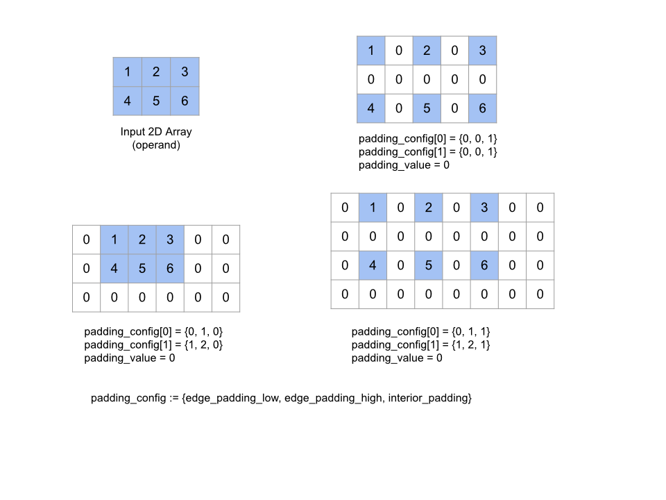
Подушка
Смотрите также XlaBuilder::Pad .
Pad(operand, padding_value, padding_config)
| Аргументы | Тип | Семантика |
|---|---|---|
operand | XlaOp | массив типа T |
padding_value | XlaOp | Скаляр типа T , чтобы заполнить добавленную прокладку |
padding_config | PaddingConfig | Сумма заполнения на обоих краях (низкий, высокий) и между элементами каждого измерения |
Расширяет заданный массив operand , пробиваясь вокруг массива, а также между элементами массива с помощью данного padding_value . padding_config Указывает количество краевой прокладки и внутренней прокладки для каждого измерения.
PaddingConfig - это повторное поле PaddingConfigDimension , которое содержит три поля для каждого измерения: edge_padding_low , edge_padding_high и interior_padding .
edge_padding_low и edge_padding_high Укажите количество заполнения, добавленное в низком уровне (рядом с индексом 0) и высококачественным (рядом с самым высоким индексом) каждого измерения соответственно. Количество краевой прокладки может быть отрицательным - абсолютное значение отрицательной прокладки указывает количество элементов для удаления из указанного измерения.
interior_padding указывает количество прокладки, добавленное между любыми двумя элементами в каждом измерении; Это не может быть негативным. Внутренняя прокладка происходит логически перед набережной, поэтому в случае отрицательной блокноты, элементы удаляются из операнда с внутренними укладками.
Эта операция является no-op, если все пары блюд с краем являются (0, 0), а значения внутренней прокладки-все 0. На рисунке ниже показаны примеры различных значений edge_padding и interior_padding для двумерного массива.
Рекв
Смотрите также XlaBuilder::Recv .
Recv(shape, channel_handle)
| Аргументы | Тип | Семантика |
|---|---|---|
shape | Shape | форма данных для получения |
channel_handle | ChannelHandle | уникальный идентификатор для каждой пары отправки/Recv |
Получает данные данной формы из инструкции Send в другом вычислении, в котором находится тот же рукояток канала. Возвращает XLAOP для полученных данных.
Клиентский API операции Recv представляет синхронную связь. Тем не менее, инструкция внутренне разложена на 2 инструкции HLO ( Recv и RecvDone ), чтобы обеспечить асинхронные передачи данных. См. Также HloInstruction::CreateRecv и HloInstruction::CreateRecvDone .
Recv(const Shape& shape, int64 channel_id)
Выделяет ресурсы, необходимые для получения данных из инструкции Send с одним и тем же каналом. Возвращает контекст для выделенных ресурсов, который используется следующей инструкцией RecvDone , чтобы дождаться завершения передачи данных. Контекст представляет собой кортеж из {полученного буфера (форма), идентификатора запроса (U32)}, и он может использоваться только инструкцией RecvDone .
RecvDone(HloInstruction context)
Учитывая контекст, созданный инструкцией Recv , ожидает завершения передачи данных и возвращает полученные данные.
Уменьшать
Смотрите также XlaBuilder::Reduce .
Применяет функцию сокращения на один или несколько массивов параллельно.
Reduce(operands..., init_values..., computation, dimensions)
| Аргументы | Тип | Семантика |
|---|---|---|
operands | Последовательность n XlaOp | N массивы типов T_0, ..., T_{N-1} . |
init_values | Последовательность n XlaOp | N скаляры типов T_0, ..., T_{N-1} . |
computation | XlaComputation | Вычисление типа T_0, ..., T_{N-1}, T_0, ..., T_{N-1} -> Collate(T_0, ..., T_{N-1}) . |
dimensions | int64 массив | Неупорядоченный массив измерений для уменьшения. |
Где:
- N должен быть больше или равен 1.
- Вычисление должно быть «примерно» ассоциативным (см. Ниже).
- Все входные массивы должны иметь одинаковые размеры.
- Все начальные значения должны сформировать идентичность в
computation. - Если
N = 1,Collate(T)- этоT. - Если
N > 1,Collate(T_0, ..., T_{N-1})-это кортежNэлементов типаT.
Эта операция уменьшает один или несколько измерений каждого входного массива на скаляры. Рангом каждого возвращенного массива является rank(operand) - len(dimensions) . Вывод OP Collate(Q_0, ..., Q_N) , где Q_i - это массив типа T_i , размеры которых описаны ниже.
Различным бэкэндам разрешено восстановить вычисление сокращения. Это может привести к численным различиям, поскольку некоторые функции восстановления, такие как добавление, не являются ассоциативными для поплавок. Однако, если диапазон данных ограничен, добавление с плавающей запятой достаточно близко к ассоциативному для большинства практических целей.
Примеры
При сокращении одного измерения в одном 1D массиве со значениями [10, 11, 12, 13] , с функцией восстановления f (это computation ), которое можно было рассчитать как
f(10, f(11, f(12, f(init_value, 13)))
Но есть и много других возможностей, например,
f(init_value, f(f(10, f(init_value, 11)), f(f(init_value, 12), f(init_value, 13))))
Ниже приведен грубый псевдокодный пример того, как может быть реализовано сокращение, используя суммирование в качестве расчета сокращения с начальным значением 0.
result_shape <- remove all dims in dimensions from operand_shape

# Iterate over all elements in result_shape. The number of r's here is equal
# to the rank of the result
for r0 in range(result_shape[0]), r1 in range(result_shape[1]), ...:
  # Initialize this result element
  result[r0, r1...] <- 0

  # Iterate over all the reduction dimensions
  for d0 in range(dimensions[0]), d1 in range(dimensions[1]), ...:
    # Increment the result element with the value of the operand's element.
    # The index of the operand's element is constructed from all ri's and di's
    # in the right order (by construction ri's and di's together index over the
    # whole operand shape).
    result[r0, r1...] += operand[ri... di]
Вот пример уменьшения 2D -массива (матрица). Форма имеет ранг 2, размер 0 размера 2 и размер 1 размера 3:
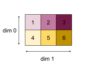
Результаты уменьшения размеров 0 или 1 с функцией «добавить»:
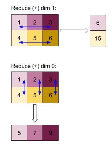
Обратите внимание, что оба результата сокращения являются 1D массивами. Диаграмма показывает один как столбец, а другой - как строка только для визуального удобства.
Для более сложного примера, вот 3D -массив. Его ранг составляет 3, измерение 0 размера 4, размер 1 размера 2 и размер 2 размера 3. Для простоты значения от 1 до 6 воспроизводятся по всему измерению 0.
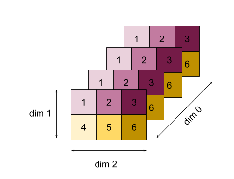
Подобно 2D -примеру, мы можем уменьшить только одно измерение. Например, если мы уменьшим размер 0, мы получим массив Rank-2, где все значения по всему измерению 0 были сложены в скаляр:
|  4   8  12 |
| 16  20  24 |
Если мы уменьшим размер 2, мы также получим массив Rank-2, где все значения по всему измерению 2 были сложены на скаляр:
| 6  15 |
| 6  15 |
| 6  15 |
| 6  15 |
Обратите внимание, что относительный порядок между оставшимися размерами на входе сохраняется на выходе, но некоторые измерения могут получить новые числа (с момента изменения ранга).
Мы также можем уменьшить несколько измерений. Дополнительные размеры 0 и 1 создают 1D массив [20, 28, 36] .
Уменьшение трехмерного массива по всем его размерам создает скаляр 84 .
Вариадический уменьшается
Когда N > 1 уменьшите функциональное приложение немного более сложное, так как оно применяется одновременно ко всем входам. Операнды поставляются в вычисление в следующем порядке:
- Запуск пониженной стоимости для первого операнда
- ...
- Запуск пониженной стоимости для N'th Operand
- Входное значение для первого операнда
- ...
- Входное значение для N'th Operand
Например, рассмотрим следующую функцию восстановления, которая может использоваться для вычисления максимального и argmax 1-D массива параллельно:
f: (Float, Int, Float, Int) -> Float, Int
f(max, argmax, value, index):
  if value >= max:
    return (value, index)
  else:
    return (max, argmax)
Для 1-D входных массивов V = Float[N], K = Int[N] и значений init I_V = Float, I_K = Int , результат f_(N-1) уменьшения в единственном входном измерении эквивалентно Следующее рекурсивное применение:
f_0 = f(I_V, I_K, V_0, K_0)
f_1 = f(f_0.first, f_0.second, V_1, K_1)
...
f_(N-1) = f(f_(N-2).first, f_(N-2).second, V_(N-1), K_(N-1))
Применение этого сокращения к массиву значений, и массив последовательных индексов (т.е. IOTA), будет сотрудничать по массивам и вернуть кортеж, содержащий максимальное значение и индекс соответствующего.
Сокращение
См. Также XlaBuilder::ReducePrecision .
Моделируют эффект преобразования значений с плавающей точкой в формат с более низким определением (например, IEEE-FP16) и обратно в исходный формат. Количество элементов и битов Mantissa в формате более низкого определения может быть указано произвольно, хотя все размеры битов не могут быть поддержаны во всех аппаратных реализациях.
ReducePrecision(operand, mantissa_bits, exponent_bits)
| Аргументы | Тип | Семантика |
|---|---|---|
operand | XlaOp | Массив типа с плавающей точкой T . |
exponent_bits | int32 | Количество бит показателей в формате с более низкой рецепцией |
mantissa_bits | int32 | Количество битов Mantissa в формате с более низкой рецепцией |
Результатом является массив типа T Входные значения округлены до ближайшего значения, представляемого данным числом битов Mantissa (с использованием «связей даже« семантики »), и любые значения, которые превышают диапазон, указанный по количеству битов, связанных с положительной или отрицательной бесконечной. Значения NaN сохраняются, хотя они могут быть преобразованы в канонические значения NaN .
Формат с более низким определением должен иметь по крайней мере один бит показателя (чтобы отличить нулевое значение от бесконечности, поскольку оба имеют нулевую мантиссу) и должны иметь неотрицательное количество битов мантиссы. Количество показателей или битов мантиссы может превышать соответствующее значение для типа T ; Соответствующая часть преобразования тогда просто не-операционная.
Восстанавливается
Смотрите также XlaBuilder::ReduceScatter .
REDUCESCATTER - это коллективная операция, которая эффективно выполняет AllReduce, а затем рассеивает результат, разделяя его на блоки shard_count вдоль scatter_dimension , а реплика i в группе реплики получает ith .
ReduceScatter(operand, computation, scatter_dim, shard_count, replica_group_ids, channel_id)
| Аргументы | Тип | Семантика |
|---|---|---|
operand | XlaOp | Массив или непустые корзины массивов, чтобы уменьшить реплики. |
computation | XlaComputation | Расчет сокращения |
scatter_dimension | int64 | Измерение, чтобы разбросить. |
shard_count | int64 | Количество блоков для разделения scatter_dimension |
replica_groups | Вектор векторов int64 | Группы, между которыми выполняются сокращения |
channel_id | Необязательный int64 | Дополнительный идентификатор канала для передачи модулей |
- Когда
operandпредставляет собой кортеж с массивами, уменьшение рассеяния выполняется на каждом элементе кортежа. -
replica_groups- это список групп реплик, между которыми выполняется сокращение (идентификатор реплики для текущей реплики может быть извлечен с использованиемReplicaId). Порядок реплик в каждой группе определяет порядок, в котором будет разбросан результат всеобъемлющего.replica_groupsдолжны быть либо пусты (в этом случае все реплики принадлежат к одной группе), либо содержать такое же количество элементов, что и количество реплик. Когда есть несколько групп реплик, все они должны быть одинакового размера. Например,replica_groups = {0, 2}, {1, 3}выполняет сокращение между репликатами0и2и1и3и затем рассеивает результат. -
shard_count- это размер каждой группы копий. Нам нужно это в тех случаях, когдаreplica_groupsпусты. Еслиreplica_groupsне пуст,shard_countдолжен быть равен размеру каждой группы реплик. -
channel_idиспользуется для передачи передачи модулей: только операцииreduce-scatterс одним и тем жеchannel_idможет общаться друг с другом.
Выходная форма - это форма ввода с scatter_dimension , сделанным shard_count Times меньше. Например, если есть две реплики, а операнд имеет значение [1.0, 2.25] и [3.0, 5.25] соответственно на две реплики, то выходное значение из этого OP, где scatter_dim - 0 , будет [4.0] для первого Реплика и [7.5] для второй копии.
Уменьшить WWINDOW
См. Также XlaBuilder::ReduceWindow .
Применяет функцию восстановления ко всем элементам в каждом окне последовательности n многомерных массивов, создавая один или кортеж из n многомерных массивов в качестве вывода. Каждый выходной массив имеет одинаковое количество элементов, что и количество допустимых позиций окна. Объединенный слой может быть выражен в виде ReduceWindow . Подобно Reduce , приложенное computation всегда передается init_values с левой стороны.
ReduceWindow(operands..., init_values..., computation, window_dimensions, window_strides, padding)
| Аргументы | Тип | Семантика |
|---|---|---|
operands | N XlaOps | Последовательность n многомерных массивов типов T_0,..., T_{N-1} , каждая из которых представляет базовую область, на которой расположено окно. |
init_values | N XlaOps | N начинающих значений для сокращения, по одному для каждого из n операндов. Смотрите уменьшить детали. |
computation | XlaComputation | Функция восстановления типа T_0, ..., T_{N-1}, T_0, ..., T_{N-1} -> Collate(T_0, ..., T_{N-1}) чтобы применить к Элементы в каждом окне всех входных операндов. |
window_dimensions | ArraySlice<int64> | массив целых чисел для значений измерений окон |
window_strides | ArraySlice<int64> | массив целых чисел для значений окон |
base_dilations | ArraySlice<int64> | массив целых чисел для базовых значений дилатации |
window_dilations | ArraySlice<int64> | массив целых чисел для значений дилатации окон |
padding | Padding | Тип заполнения для окна (Padding :: ksame, которая накладывает такую же форму выходной формы, что и вход, если шаг составляет 1 или накладка :: kvalid, который не использует прокладки и «останавливает» окно, как только он больше не подходит) |
Где:
- N должен быть больше или равен 1.
- Все входные массивы должны иметь одинаковые размеры.
- Если
N = 1,Collate(T)- этоT. - Если
N > 1,Collate(T_0, ..., T_{N-1})-это кортежNэлементов типа(T0,...T{N-1}).
Ниже код и рисунок показан пример использования ReduceWindow . Ввод - это матрица размера [4x6], а как window_dimensions, так и window_stride_dimensions [2x3].
// Create a computation for the reduction (maximum).
XlaComputation max;
{
  XlaBuilder builder(client_, "max");
  auto y = builder.Parameter(0, ShapeUtil::MakeShape(F32, {}), "y");
  auto x = builder.Parameter(1, ShapeUtil::MakeShape(F32, {}), "x");
  builder.Max(y, x);
  max = builder.Build().value();
}

// Create a ReduceWindow computation with the max reduction computation.
XlaBuilder builder(client_, "reduce_window_2x3");
auto shape = ShapeUtil::MakeShape(F32, {4, 6});
auto input = builder.Parameter(0, shape, "input");
builder.ReduceWindow(
    input,
    /*init_val=*/builder.ConstantLiteral(LiteralUtil::MinValue(F32)),
    *max,
    /*window_dimensions=*/{2, 3},
    /*window_stride_dimensions=*/{2, 3},
    Padding::kValid);
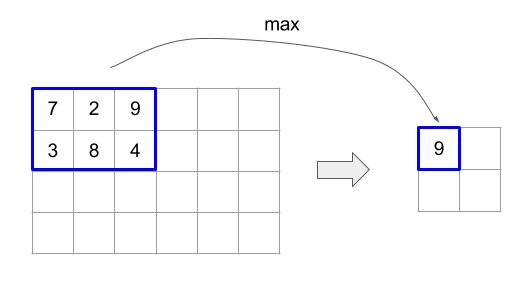
Шаг 1 в измерении указывает, что положение окна в измерении составляет 1 элемент от его соседнего окна. Чтобы указать, что ни одно окна перекрывается друг с другом, Window_stride_dimensions должен быть равным Window_dimensions. Рисунок ниже иллюстрирует использование двух разных значений шага. Padding is applied to each dimension of the input and the calculations are the same as though the input came in with the dimensions it has after padding.
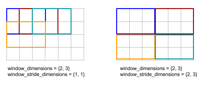
For a non-trivial padding example, consider computing reduce-window minimum (initial value is MAX_FLOAT ) with dimension 3 and stride 2 over the input array [10000, 1000, 100, 10, 1] . Padding kValid computes minimums over two valid windows: [10000, 1000, 100] and [100, 10, 1] , resulting in the output [100, 1] . Padding kSame first pads the array so that the shape after the reduce-window would be the same as input for stride one by adding initial elements on both sides, getting [MAX_VALUE, 10000, 1000, 100, 10, 1, MAX_VALUE] . Running reduce-window over the padded array operates on three windows [MAX_VALUE, 10000, 1000] , [1000, 100, 10] , [10, 1, MAX_VALUE] , and yields [1000, 10, 1] .
The evaluation order of the reduction function is arbitrary and may be non-deterministic. Therefore, the reduction function should not be overly sensitive to reassociation. See the discussion about associativity in the context of Reduce for more details.
ReplicaId
See also XlaBuilder::ReplicaId .
Returns the unique ID (U32 scalar) of the replica.
ReplicaId()
The unique ID of each replica is an unsigned integer in the interval [0, N) , where N is the number of replicas. Since all the replicas are running the same program, a ReplicaId() call in the program will return a different value on each replica.
Изменить форму
See also XlaBuilder::Reshape and the Collapse operation.
Reshapes the dimensions of an array into a new configuration.
Reshape(operand, new_sizes) Reshape(operand, dimensions, new_sizes)
| Аргументы | Тип | Семантика |
|---|---|---|
operand | XlaOp | array of type T |
dimensions | int64 vector | order in which dimensions are collapsed |
new_sizes | int64 vector | vector of sizes of new dimensions |
Conceptually, reshape first flattens an array into a one-dimensional vector of data values, and then refines this vector into a new shape. The input arguments are an arbitrary array of type T, a compile-time-constant vector of dimension indices, and a compile-time-constant vector of dimension sizes for the result. The values in the dimension vector, if given, must be a permutation of all of T's dimensions; the default if not given is {0, ..., rank - 1} . The order of the dimensions in dimensions is from slowest-varying dimension (most major) to fastest-varying dimension (most minor) in the loop nest which collapses the input array into a single dimension. The new_sizes vector determines the size of the output array. The value at index 0 in new_sizes is the size of dimension 0, the value at index 1 is the size of dimension 1, and so on. The product of the new_size dimensions must equal the product of the operand's dimension sizes. When refining the collapsed array into the multidimensional array defined by new_sizes , the dimensions in new_sizes are ordered from slowest varying (most major) and to fastest varying (most minor).
For example, let v be an array of 24 elements:
let v = f32[4x2x3] { { {10, 11, 12}, {15, 16, 17} },
                    { {20, 21, 22}, {25, 26, 27} },
                    { {30, 31, 32}, {35, 36, 37} },
                    { {40, 41, 42}, {45, 46, 47} } };

In-order collapse:
let v012_24 = Reshape(v, {0,1,2}, {24});
then v012_24 == f32[24] {10, 11, 12, 15, 16, 17, 20, 21, 22, 25, 26, 27,
                         30, 31, 32, 35, 36, 37, 40, 41, 42, 45, 46, 47};

let v012_83 = Reshape(v, {0,1,2}, {8,3});
then v012_83 == f32[8x3] { {10, 11, 12}, {15, 16, 17},
                          {20, 21, 22}, {25, 26, 27},
                          {30, 31, 32}, {35, 36, 37},
                          {40, 41, 42}, {45, 46, 47} };

Out-of-order collapse:
let v021_24 = Reshape(v, {1,2,0}, {24});
then v012_24 == f32[24]  {10, 20, 30, 40, 11, 21, 31, 41, 12, 22, 32, 42,
                          15, 25, 35, 45, 16, 26, 36, 46, 17, 27, 37, 47};

let v021_83 = Reshape(v, {1,2,0}, {8,3});
then v021_83 == f32[8x3] { {10, 20, 30}, {40, 11, 21},
                          {31, 41, 12}, {22, 32, 42},
                          {15, 25, 35}, {45, 16, 26},
                          {36, 46, 17}, {27, 37, 47} };


let v021_262 = Reshape(v, {1,2,0}, {2,6,2});
then v021_262 == f32[2x6x2] { { {10, 20}, {30, 40},
                              {11, 21}, {31, 41},
                              {12, 22}, {32, 42} },
                             { {15, 25}, {35, 45},
                              {16, 26}, {36, 46},
                              {17, 27}, {37, 47} } };
As a special case, reshape can transform a single-element array to a scalar and vice versa. Например,
Reshape(f32[1x1] { {5} }, {0,1}, {}) == 5;
Reshape(5, {}, {1,1}) == f32[1x1] { {5} };
Rev (reverse)
See also XlaBuilder::Rev .
Rev(operand, dimensions)
| Аргументы | Тип | Семантика |
|---|---|---|
operand | XlaOp | array of type T |
dimensions | ArraySlice<int64> | dimensions to reverse |
Reverses the order of elements in the operand array along the specified dimensions , generating an output array of the same shape. Each element of the operand array at a multidimensional index is stored into the output array at a transformed index. The multidimensional index is transformed by reversing the index in each dimension to be reversed (ie, if a dimension of size N is one of the reversing dimensions, its index i is transformed into N - 1 - i).
One use for the Rev operation is to reverse the convolution weight array along the two window dimensions during the gradient computation in neural networks.
RngNormal
See also XlaBuilder::RngNormal .
Constructs an output of a given shape with random numbers generated following the \(N(\mu, \sigma)\) normal distribution. The parameters \(\mu\) and \(\sigma\), and output shape have to have a floating point elemental type. The parameters furthermore have to be scalar valued.
RngNormal(mu, sigma, shape)
| Аргументы | Тип | Семантика |
|---|---|---|
mu | XlaOp | Scalar of type T specifying mean of generated numbers |
sigma | XlaOp | Scalar of type T specifying standard deviation of generated |
shape | Shape | Output shape of type T |
RngUniform
See also XlaBuilder::RngUniform .
Constructs an output of a given shape with random numbers generated following the uniform distribution over the interval \([a,b)\). The parameters and output element type have to be a boolean type, an integral type or a floating point types, and the types have to be consistent. The CPU and GPU backends currently only support F64, F32, F16, BF16, S64, U64, S32 and U32. Furthermore, the parameters need to be scalar valued. If \(b <= a\) the result is implementation-defined.
RngUniform(a, b, shape)
| Аргументы | Тип | Семантика |
|---|---|---|
a | XlaOp | Scalar of type T specifying lower limit of interval |
b | XlaOp | Scalar of type T specifying upper limit of interval |
shape | Shape | Output shape of type T |
RngBitGenerator
Generates an output with a given shape filled with uniform random bits using the specified algorithm (or backend default) and returns an updated state (with the same shape as initial state) and the generated random data.
Initial state is the initial state of the current random number generation. It and the required shape and valid values are dependent on the algorithm used.
The output is guaranteed to be a deterministic function of the initial state but it is not guaranteed to be deterministic between backends and different compiler versions.
RngBitGenerator(algorithm, key, shape)
| Аргументы | Тип | Семантика |
|---|---|---|
algorithm | RandomAlgorithm | PRNG algorithm to be used. |
initial_state | XlaOp | Initial state for the PRNG algorithm. |
shape | Shape | Output shape for generated data. |
Available values for algorithm :
rng_default: Backend specific algorithm with backend specific shape requirements.rng_three_fry: ThreeFry counter-based PRNG algorithm. Theinitial_stateshape isu64[2]with arbitrary values. Салмон и др. SC 2011. Parallel random numbers: as easy as 1, 2, 3.rng_philox: Philox algorithm to generate random numbers in parallel. Theinitial_stateshape isu64[3]with arbitrary values. Салмон и др. SC 2011. Parallel random numbers: as easy as 1, 2, 3.
Разброс
The XLA scatter operation generates a sequence of results which are the values of the input array operands , with several slices (at indices specified by scatter_indices ) updated with the sequence of values in updates using update_computation .
See also XlaBuilder::Scatter .
scatter(operands..., scatter_indices, updates..., update_computation, index_vector_dim, update_window_dims, inserted_window_dims, scatter_dims_to_operand_dims)
| Аргументы | Тип | Семантика |
|---|---|---|
operands | Sequence of N XlaOp | N arrays of types T_0, ..., T_N to be scattered into. |
scatter_indices | XlaOp | Array containing the starting indices of the slices that must be scattered to. |
updates | Sequence of N XlaOp | N arrays of types T_0, ..., T_N . updates[i] contains the values that must be used for scattering operands[i] . |
update_computation | XlaComputation | Computation to be used for combining the existing values in the input array and the updates during scatter. This computation should be of type T_0, ..., T_N, T_0, ..., T_N -> Collate(T_0, ..., T_N) . |
index_vector_dim | int64 | The dimension in scatter_indices that contains the starting indices. |
update_window_dims | ArraySlice<int64> | The set of dimensions in updates shape that are window dimensions . |
inserted_window_dims | ArraySlice<int64> | The set of window dimensions that must be inserted into updates shape. |
scatter_dims_to_operand_dims | ArraySlice<int64> | A dimensions map from the scatter indices to the operand index space. This array is interpreted as mapping i to scatter_dims_to_operand_dims[i] . It has to be one-to-one and total. |
indices_are_sorted | bool | Whether the indices are guaranteed to be sorted by the caller. |
Где:
- N is required to be greater or equal to 1.
-
operands[0], ...,operands[N-1] must all have the same dimensions. -
updates[0], ...,updates[N-1] must all have the same dimensions. - If
N = 1,Collate(T)isT. - If
N > 1,Collate(T_0, ..., T_N)is a tuple ofNelements of typeT.
If index_vector_dim is equal to scatter_indices.rank we implicitly consider scatter_indices to have a trailing 1 dimension.
We define update_scatter_dims of type ArraySlice<int64> as the set of dimensions in updates shape that are not in update_window_dims , in ascending order.
The arguments of scatter should follow these constraints:
Each
updatesarray must be of rankupdate_window_dims.size + scatter_indices.rank - 1.Bounds of dimension
iin eachupdatesarray must conform to the following:- If
iis present inupdate_window_dims(ie equal toupdate_window_dims[k] for somek), then the bound of dimensioniinupdatesmust not exceed the corresponding bound ofoperandafter accounting for theinserted_window_dims(ieadjusted_window_bounds[k], whereadjusted_window_boundscontains the bounds ofoperandwith the bounds at indicesinserted_window_dimsremoved). - If
iis present inupdate_scatter_dims(ie equal toupdate_scatter_dims[k] for somek), then the bound of dimensioniinupdatesmust be equal to the corresponding bound ofscatter_indices, skippingindex_vector_dim(iescatter_indices.shape.dims[k], ifk<index_vector_dimandscatter_indices.shape.dims[k+1] otherwise).
- If
update_window_dimsmust be in ascending order, not have any repeating dimension numbers, and be in the range[0, updates.rank).inserted_window_dimsmust be in ascending order, not have any repeating dimension numbers, and be in the range[0, operand.rank).operand.rankmust equal the sum ofupdate_window_dims.sizeandinserted_window_dims.size.scatter_dims_to_operand_dims.sizemust be equal toscatter_indices.shape.dims[index_vector_dim], and its values must be in the range[0, operand.rank).
For a given index U in each updates array, the corresponding index I in the corresponding operands array into which this update has to be applied is computed as follows:
- Let
G= {U[k] forkinupdate_scatter_dims}. UseGto look up an index vectorSin thescatter_indicesarray such thatS[i] =scatter_indices[Combine(G,i)] where Combine(A, b) inserts b at positionsindex_vector_diminto A. - Create an index
SinintooperandusingSby scatteringSusing thescatter_dims_to_operand_dimsmap. More formally:-
Sin[scatter_dims_to_operand_dims[k]] =S[k] ifk<scatter_dims_to_operand_dims.size. -
Sin[_] =0otherwise.
-
- Create an index
Wininto eachoperandsarray by scattering the indices atupdate_window_dimsinUaccording toinserted_window_dims. More formally:-
Win[window_dims_to_operand_dims(k)] =U[k] ifkis inupdate_window_dims, wherewindow_dims_to_operand_dimsis the monotonic function with domain [0,update_window_dims.size) and range [0,operand.rank) \inserted_window_dims. (For example, ifupdate_window_dims.sizeis4,operand.rankis6, andinserted_window_dimsis {0,2} thenwindow_dims_to_operand_dimsis {0→1,1→3,2→4,3→5}). -
Win[_] =0otherwise.
-
-
IisWin+Sinwhere + is element-wise addition.
In summary, the scatter operation can be defined as follows.
- Initialize
outputwithoperands, ie for all indicesJ, for all indicesOin theoperands[J] array:
output[J][O] =operands[J][O] - For every index
Uin theupdates[J] array and the corresponding indexOin theoperand[J] array, ifOis a valid index foroutput:
(output[0][O], ...,output[N-1][O]) =update_computation(output[0][O], ..., ,output[N-1][O],updates[0][U], ...,updates[N-1][U])
The order in which updates are applied is non-deterministic. So, when multiple indices in updates refer to the same index in operands , the corresponding value in output will be non-deterministic.
Note that the first parameter that is passed into the update_computation will always be the current value from the output array and the second parameter will always be the value from the updates array. This is important specifically for cases when the update_computation is not commutative .
If indices_are_sorted is set to true then XLA can assume that start_indices are sorted (in ascending start_index_map order) by the user. If they are not then the semantics is implementation defined.
Informally, the scatter op can be viewed as an inverse of the gather op, ie the scatter op updates the elements in the input that are extracted by the corresponding gather op.
For a detailed informal description and examples, refer to the "Informal Description" section under Gather .
Выбирать
See also XlaBuilder::Select .
Constructs an output array from elements of two input arrays, based on the values of a predicate array.
Select(pred, on_true, on_false)
| Аргументы | Тип | Семантика |
|---|---|---|
pred | XlaOp | array of type PRED |
on_true | XlaOp | array of type T |
on_false | XlaOp | array of type T |
The arrays on_true and on_false must have the same shape. This is also the shape of the output array. The array pred must have the same dimensionality as on_true and on_false , with the PRED element type.
For each element P of pred , the corresponding element of the output array is taken from on_true if the value of P is true , and from on_false if the value of P is false . As a restricted form of broadcasting , pred can be a scalar of type PRED . In this case, the output array is taken wholly from on_true if pred is true , and from on_false if pred is false .
Example with non-scalar pred :
let pred: PRED[4] = {true, false, false, true};
let v1: s32[4] = {1, 2, 3, 4};
let v2: s32[4] = {100, 200, 300, 400};
==>
Select(pred, v1, v2) = s32[4]{1, 200, 300, 4};
Example with scalar pred :
let pred: PRED = true;
let v1: s32[4] = {1, 2, 3, 4};
let v2: s32[4] = {100, 200, 300, 400};
==>
Select(pred, v1, v2) = s32[4]{1, 2, 3, 4};
Selections between tuples are supported. Tuples are considered to be scalar types for this purpose. If on_true and on_false are tuples (which must have the same shape!) then pred has to be a scalar of type PRED .
SelectAndScatter
See also XlaBuilder::SelectAndScatter .
This operation can be considered as a composite operation that first computes ReduceWindow on the operand array to select an element from each window, and then scatters the source array to the indices of the selected elements to construct an output array with the same shape as the operand множество. The binary select function is used to select an element from each window by applying it across each window, and it is called with the property that the first parameter's index vector is lexicographically less than the second parameter's index vector. The select function returns true if the first parameter is selected and returns false if the second parameter is selected, and the function must hold transitivity (ie, if select(a, b) and select(b, c) are true , then select(a, c) is also true ) so that the selected element does not depend on the order of the elements traversed for a given window.
The function scatter is applied at each selected index in the output array. It takes two scalar parameters:
- Current value at the selected index in the output array
- The scatter value from
sourcethat applies to the selected index
It combines the two parameters and returns a scalar value that's used to update the value at the selected index in the output array. Initially, all indices of the output array are set to init_value .
The output array has the same shape as the operand array and the source array must have the same shape as the result of applying a ReduceWindow operation on the operand array. SelectAndScatter can be used to backpropagate the gradient values for a pooling layer in a neural network.
SelectAndScatter(operand, select, window_dimensions, window_strides, padding, source, init_value, scatter)
| Аргументы | Тип | Семантика |
|---|---|---|
operand | XlaOp | array of type T over which the windows slide |
select | XlaComputation | binary computation of type T, T -> PRED , to apply to all elements in each window; returns true if the first parameter is selected and returns false if the second parameter is selected |
window_dimensions | ArraySlice<int64> | array of integers for window dimension values |
window_strides | ArraySlice<int64> | array of integers for window stride values |
padding | Padding | padding type for window (Padding::kSame or Padding::kValid) |
source | XlaOp | array of type T with the values to scatter |
init_value | XlaOp | scalar value of type T for the initial value of the output array |
scatter | XlaComputation | binary computation of type T, T -> T , to apply each scatter source element with its destination element |
The figure below shows examples of using SelectAndScatter , with the select function computing the maximal value among its parameters. Note that when the windows overlap, as in the figure (2) below, an index of the operand array may be selected multiple times by different windows. In the figure, the element of value 9 is selected by both of the top windows (blue and red) and the binary addition scatter function produces the output element of value 8 (2 + 6).
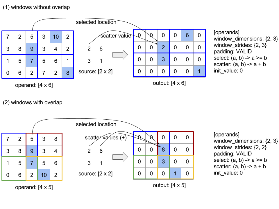
The evaluation order of the scatter function is arbitrary and may be non-deterministic. Therefore, the scatter function should not be overly sensitive to reassociation. See the discussion about associativity in the context of Reduce for more details.
Отправлять
See also XlaBuilder::Send .
Send(operand, channel_handle)
| Аргументы | Тип | Семантика |
|---|---|---|
operand | XlaOp | data to send (array of type T) |
channel_handle | ChannelHandle | unique identifier for each send/recv pair |
Sends the given operand data to a Recv instruction in another computation that shares the same channel handle. Does not return any data.
Similar to the Recv operation, the client API of Send operation represents synchronous communication, and is internally decomposed into 2 HLO instructions ( Send and SendDone ) to enable asynchronous data transfers. See also HloInstruction::CreateSend and HloInstruction::CreateSendDone .
Send(HloInstruction operand, int64 channel_id)
Initiates an asynchronous transfer of the operand to the resources allocated by the Recv instruction with the same channel id. Returns a context, which is used by a following SendDone instruction to wait for the completion of the data transfer. The context is a tuple of {operand (shape), request identifier (U32)} and it can only be used by a SendDone instruction.
SendDone(HloInstruction context)
Given a context created by a Send instruction, waits for the data transfer to complete. The instruction does not return any data.
Scheduling of channel instructions
The execution order of the 4 instructions for each channel ( Recv , RecvDone , Send , SendDone ) is as below.
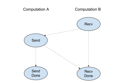
-
Recvhappens beforeSend -
Sendhappens beforeRecvDone -
Recvhappens beforeRecvDone -
Sendhappens beforeSendDone
When the backend compilers generate a linear schedule for each computation that communicates via channel instructions, there must not be cycles across the computations. For example, below schedules lead to deadlocks.
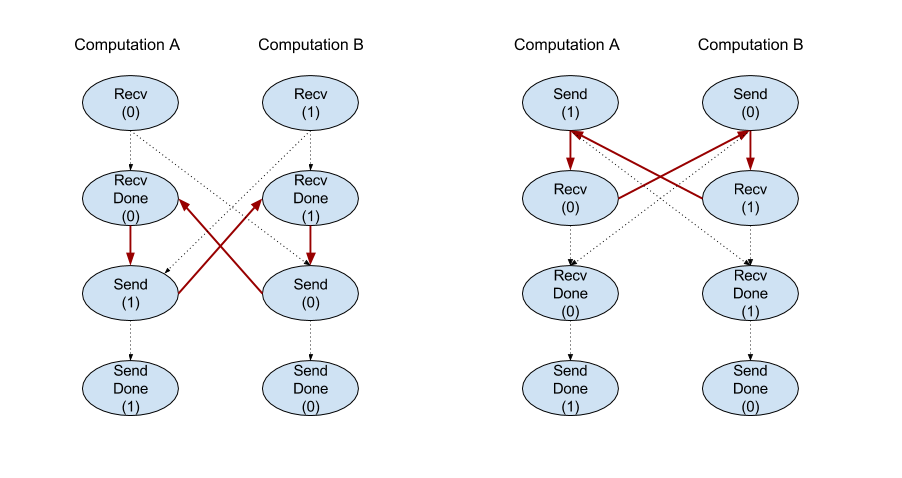
Кусочек
See also XlaBuilder::Slice .
Slicing extracts a sub-array from the input array. The sub-array is of the same rank as the input and contains the values inside a bounding box within the input array where the dimensions and indices of the bounding box are given as arguments to the slice operation.
Slice(operand, start_indices, limit_indices, strides)
| Аргументы | Тип | Семантика |
|---|---|---|
operand | XlaOp | N dimensional array of type T |
start_indices | ArraySlice<int64> | List of N integers containing the starting indices of the slice for each dimension. Values must be greater than or equal to zero. |
limit_indices | ArraySlice<int64> | List of N integers containing the ending indices (exclusive) for the slice for each dimension. Each value must be greater than or equal to the respective start_indices value for the dimension and less than or equal to the size of the dimension. |
strides | ArraySlice<int64> | List of N integers that decides the input stride of the slice. The slice picks every strides[d] element in dimension d . |
1-dimensional example:
let a = {0.0, 1.0, 2.0, 3.0, 4.0}
Slice(a, {2}, {4}) produces:
  {2.0, 3.0}
2-dimensional example:
let b =
 { {0.0,  1.0,  2.0},
   {3.0,  4.0,  5.0},
   {6.0,  7.0,  8.0},
   {9.0, 10.0, 11.0} }

Slice(b, {2, 1}, {4, 3}) produces:
  { { 7.0,  8.0},
    {10.0, 11.0} }
Сортировать
See also XlaBuilder::Sort .
Sort(operands, comparator, dimension, is_stable)
| Аргументы | Тип | Семантика |
|---|---|---|
operands | ArraySlice<XlaOp> | The operands to sort. |
comparator | XlaComputation | The comparator computation to use. |
dimension | int64 | The dimension along which to sort. |
is_stable | bool | Whether stable sorting should be used. |
If only one operand is provided:
If the operand is a rank-1 tensor (an array), the result is a sorted array. If you want to sort the array into ascending order, the comparator should perform a less-than comparison. Formally, after the array is sorted, it holds for all index positions
i, jwithi < jthat eithercomparator(value[i], value[j]) = comparator(value[j], value[i]) = falseorcomparator(value[i], value[j]) = true.If the operand has higher rank, the operand is sorted along the provided dimension. For example, for a rank-2 tensor (a matrix), a dimension value of
0will independently sort every column, and a dimension value of1will independently sort each row. If no dimension number is provided, then the last dimension is chosen by default. For the dimension which is sorted, the same sorting order applies as in the rank-1 case.
If n > 1 operands are provided:
All
noperands must be tensors with the same dimensions. The element types of the tensors may be different.All operands are sorted together, not individually. Conceptually the operands are treated as a tuple. When checking whether the elements of each operand at index positions
iandjneed to be swapped, the comparator is called with2 * nscalar parameters, where parameter2 * kcorresponds to the value at positionifrom thek-thoperand, and parameter2 * k + 1corresponds to the value at positionjfrom thek-thoperand. Usually, the comparator would thus compare parameters2 * kand2 * k + 1with each other and possibly use other parameter pairs as tie breakers.The result is a tuple that consists of the operands in sorted order (along the provided dimension, as above). The
i-thoperand of the tuple corresponds to thei-thoperand of Sort.
For example, if there are three operands operand0 = [3, 1] , operand1 = [42, 50] , operand2 = [-3.0, 1.1] , and the comparator compares only the values of operand0 with less-than, then the output of the sort is the tuple ([1, 3], [50, 42], [1.1, -3.0]) .
If is_stable is set to true, the sort is guaranteed to be stable, that is, if there are elements which are considered to be equal by the comparator, the relative order of the equal values is preserved. Two elements e1 and e2 are equal if and only if comparator(e1, e2) = comparator(e2, e1) = false . By default, is_stable is set to false.
Транспонировать
See also the tf.reshape operation.
Transpose(operand)
| Аргументы | Тип | Семантика |
|---|---|---|
operand | XlaOp | The operand to transpose. |
permutation | ArraySlice<int64> | How to permute the dimensions. |
Permutes the operand dimensions with the given permutation, so ∀ i . 0 ≤ i < rank ⇒ input_dimensions[permutation[i]] = output_dimensions[i] .
This is the same as Reshape(operand, permutation, Permute(permutation, operand.shape.dimensions)).
TriangularSolve
See also XlaBuilder::TriangularSolve .
Solves systems of linear equations with lower or upper triangular coefficient matrices by forward- or back-substitution. Broadcasting along leading dimensions, this routine solves one of the matrix systems op(a) * x = b , or x * op(a) = b , for the variable x , given a and b , where op(a) is either op(a) = a , or op(a) = Transpose(a) , or op(a) = Conj(Transpose(a)) .
TriangularSolve(a, b, left_side, lower, unit_diagonal, transpose_a)
| Аргументы | Тип | Семантика |
|---|---|---|
a | XlaOp | a rank > 2 array of a complex or floating-point type with shape [..., M, M] . |
b | XlaOp | a rank > 2 array of the same type with shape [..., M, K] if left_side is true, [..., K, M] otherwise. |
left_side | bool | indicates whether to solve a system of the form op(a) * x = b ( true ) or x * op(a) = b ( false ). |
lower | bool | whether to use the upper or lower triangle of a . |
unit_diagonal | bool | if true , the diagonal elements of a are assumed to be 1 and not accessed. |
transpose_a | Transpose | whether to use a as is, transpose it or take its conjugate transpose. |
Input data is read only from the lower/upper triangle of a , depending on the value of lower . Values from the other triangle are ignored. Output data is returned in the same triangle; the values in the other triangle are implementation-defined and may be anything.
If the rank of a and b are greater than 2, they are treated as batches of matrices, where all except the minor 2 dimensions are batch dimensions. a and b must have equal batch dimensions.
Кортеж
See also XlaBuilder::Tuple .
A tuple containing a variable number of data handles, each of which has its own shape.
This is analogous to std::tuple in C++. Концептуально:
let v: f32[10] = f32[10]{0, 1, 2, 3, 4, 5, 6, 7, 8, 9};
let s: s32 = 5;
let t: (f32[10], s32) = tuple(v, s);
Tuples can be deconstructed (accessed) via the GetTupleElement operation.
Пока
See also XlaBuilder::While .
While(condition, body, init)
| Аргументы | Тип | Семантика |
|---|---|---|
condition | XlaComputation | XlaComputation of type T -> PRED which defines the termination condition of theloop. |
body | XlaComputation | XlaComputation of type T -> T which defines the body of the loop. |
init | T | Initial value for the parameter of condition and body . |
Sequentially executes the body until the condition fails. This is similar to a typical while loop in many other languages except for the differences and restrictions listed below.
- A
Whilenode returns a value of typeT, which is the result from the last execution of thebody. - The shape of the type
Tis statically determined and must be the same across all iterations.
The T parameters of the computations are initialized with the init value in the first iteration and are automatically updated to the new result from body in each subsequent iteration.
One main use case of the While node is to implement the repeated execution of training in neural networks. Simplified pseudocode is shown below with a graph that represents the computation. The code can be found in while_test.cc . The type T in this example is a Tuple consisting of an int32 for the iteration count and a vector[10] for the accumulator. For 1000 iterations, the loop keeps adding a constant vector to the accumulator.
// Pseudocode for the computation.
init = {0, zero_vector[10]} // Tuple of int32 and float[10].
result = init;
while (result(0) < 1000) {
  iteration = result(0) + 1;
  new_vector = result(1) + constant_vector[10];
  result = {iteration, new_vector};
}