ต่อไปนี้เป็นคำอธิบายความหมายของการดำเนินการที่กำหนดไว้ในอินเทอร์เฟซ XlaBuilder โดยปกติแล้ว การดำเนินการเหล่านี้จะแมปแบบหนึ่งต่อหนึ่งกับการดำเนินการที่กำหนดไว้ในอินเทอร์เฟซ RPC ใน xla_data.proto
หมายเหตุเกี่ยวกับการตั้งชื่อ: ประเภทข้อมูลทั่วไปที่ XLA ตกลงด้วยคืออาร์เรย์ N มิติที่มีองค์ประกอบของประเภทแบบเดียวกันบางอย่าง (เช่น ทศนิยม 32 บิต) ตลอดทั้งเอกสารประกอบจะใช้ array เพื่อแสดงอาร์เรย์ตามมิติข้อมูลที่กำหนดเอง เพื่อความสะดวก กรณีพิเศษจะมีชื่อที่เจาะจงและคุ้นเคยมากกว่า เช่น เวกเตอร์คืออาร์เรย์ 1 มิติ และเมทริกซ์คืออาร์เรย์ 2 มิติ
AfterAll
ดู XlaBuilder::AfterAll เพิ่มเติม
AfterAll จะใช้โทเค็นจำนวนหนึ่งและสร้างโทเค็นเดียว โทเค็นเป็นประเภทพื้นฐานซึ่งนำมาเรียงต่อกันระหว่างการดำเนินการที่ทำให้เกิดผลข้างเคียงเพื่อบังคับใช้การเรียงลำดับ AfterAll จะใช้เป็นการรวมโทเค็นเพื่อเรียงลำดับการดำเนินการหลังจากการดำเนินการที่ตั้งค่าไว้ได้
AfterAll(operands)
| อาร์กิวเมนต์ | ประเภท | อรรถศาสตร์ |
|---|---|---|
operands |
XlaOp |
จำนวนโทเค็นที่แตกต่างกัน |
AllGather
ดู XlaBuilder::AllGather เพิ่มเติม
ดำเนินการเชื่อมต่อตัวจำลองต่างๆ
AllGather(operand, all_gather_dim, shard_count, replica_group_ids,
channel_id)
| อาร์กิวเมนต์ | ประเภท | อรรถศาสตร์ |
|---|---|---|
operand
|
XlaOp
|
อาร์เรย์เพื่อต่อข้อมูลจำลอง |
all_gather_dim |
int64 |
มิติข้อมูลการต่อกัน |
replica_groups
|
เวกเตอร์ของเวกเตอร์ของ
int64 |
กลุ่มที่ใช้เชื่อมต่อ |
channel_id
|
ไม่บังคับ int64
|
รหัสแชแนลที่ไม่บังคับสำหรับ การสื่อสารข้ามโมดูล |
replica_groupsคือรายการของกลุ่มตัวจำลองที่จะมีการต่อข้อมูล (จะดึงข้อมูลรหัสการจำลองสำหรับตัวจำลองปัจจุบันได้โดยใช้ReplicaId) ลำดับของตัวจำลองในแต่ละกลุ่มจะเป็นตัวกำหนดลำดับอินพุตของอินพุตในผลลัพธ์replica_groupsต้องว่างเปล่า (ในกรณีนี้ตัวจำลองทั้งหมดจะเป็นของกลุ่มเดียว โดยเรียงลำดับจาก0ถึงN - 1) หรือมีจำนวนองค์ประกอบเท่ากับจำนวนตัวจำลอง ตัวอย่างเช่นreplica_groups = {0, 2}, {1, 3}จะเชื่อมต่อตัวจำลอง0กับ2รวมถึง1กับ3shard_countคือขนาดของกลุ่มตัวจำลองแต่ละกลุ่ม เราต้องการข้อมูลนี้ในกรณีที่replica_groupsว่างเปล่าchannel_idใช้สำหรับการสื่อสารข้ามโมดูล: มีเพียงall-gatherการดำเนินการที่มีchannel_idเดียวกันเท่านั้นที่สื่อสารกันได้
รูปร่างเอาต์พุตเป็นรูปร่างอินพุตที่มี all_gather_dim ทำให้ใหญ่ขึ้น shard_count เท่า เช่น หากมีตัวจำลอง 2 รายการและตัวถูกดำเนินการมีค่า [1.0, 2.5] และ [3.0, 5.25] ตามลำดับในตัวจำลอง 2 ตัว ค่าเอาต์พุตจากตัวจำลองนี้ที่ all_gather_dim คือ 0 จะเป็น [1.0, 2.5, 3.0,
5.25] สำหรับตัวจำลองทั้ง 2 รายการ
AllReduce
ดู XlaBuilder::AllReduce เพิ่มเติม
ดำเนินการคำนวณแบบกำหนดเองกับตัวจำลองต่างๆ
AllReduce(operand, computation, replica_group_ids, channel_id)
| อาร์กิวเมนต์ | ประเภท | อรรถศาสตร์ |
|---|---|---|
operand
|
XlaOp
|
อาร์เรย์หรือ Tuple ของอาร์เรย์ที่ไม่ว่างเปล่าเพื่อลดขนาดของตัวจำลอง |
computation |
XlaComputation |
การคํานวณการลด |
replica_groups
|
เวกเตอร์ของเวกเตอร์ของ
int64 |
กลุ่มที่ใช้การลด |
channel_id
|
ไม่บังคับ int64
|
รหัสแชแนลที่ไม่บังคับสำหรับ การสื่อสารข้ามโมดูล |
- เมื่อ
operandเป็น Tuple ของอาร์เรย์ ระบบจะดำเนินการลดทั้งหมดกับแต่ละองค์ประกอบของ Tuple replica_groupsคือรายการของกลุ่มตัวจำลองที่ใช้ทำการลด (สามารถเรียกข้อมูลรหัสการจำลองสำหรับตัวจำลองปัจจุบันได้โดยใช้ReplicaId)replica_groupsต้องว่างเปล่า (ในกรณีที่ตัวจำลองทั้งหมดอยู่ในกลุ่มเดียว) หรือมีจำนวนองค์ประกอบเท่ากับจำนวนตัวจำลอง ตัวอย่างเช่นreplica_groups = {0, 2}, {1, 3}จะลดจำนวนตัวจำลอง0กับ2และ1กับ3channel_idใช้สำหรับการสื่อสารข้ามโมดูล: มีเพียงall-reduceการดำเนินการที่มีchannel_idเดียวกันเท่านั้นที่สื่อสารกันได้
รูปร่างเอาต์พุตจะเหมือนกับรูปร่างอินพุต เช่น หากมีตัวจำลอง 2 รายการและตัวถูกดำเนินการมีค่า [1.0, 2.5] และ [3.0, 5.25] ตามลำดับบนตัวจำลองทั้ง 2 ตัว ค่าเอาต์พุตจากการคํานวณ op และผลรวมจะเท่ากับ [4.0, 7.75] บนตัวจำลองทั้ง 2 รายการ หากอินพุตเป็น Tuple เอาต์พุตจะเป็น Tuple เช่นกัน
การคำนวณผลลัพธ์ของ AllReduce ต้องมีอินพุต 1 รายการจากตัวจำลองแต่ละตัว ดังนั้นหากตัวจำลองตัวหนึ่งเรียกใช้โหนด AllReduce มากกว่าอีกอันหนึ่ง ตัวจำลองเดิมจะรอตลอดไป เนื่องจากตัวจำลองต่างก็เรียกใช้โปรแกรมเดียวกัน จึงมีวิธีดำเนินการไม่มากนัก แต่ก็เป็นไปได้หากเงื่อนไขของลูปขึ้นอยู่กับข้อมูลจาก InFeed และข้อมูลที่ป้อนเข้ามาทำให้มีการวนซ้ำขณะทำซ้ำบนตัวจำลองตัวหนึ่งมากกว่าอีกตัวหนึ่ง
AllToAll
ดู XlaBuilder::AllToAll เพิ่มเติม
AllToAll คือการดำเนินการร่วมที่ส่งข้อมูลจากแกนทั้งหมดไปยังแกนทั้งหมด โดยมี 2 ระยะ ดังนี้
- ระยะกระจาย ในแต่ละแกน ตัวถูกดำเนินการจะแบ่งออกเป็น
split_countบล็อกตามsplit_dimensionsและบล็อกจะกระจายไปยังแกนทั้งหมด เช่น ส่งบล็อก ith ไปยังแกน ith - ระยะการรวบรวม แกนประมวลผลแต่ละรายการจะเชื่อมบล็อกที่ได้รับตามแนว
concat_dimension
แกนที่เข้าร่วมจะกำหนดค่าได้โดย
replica_groups: ReplicaGroup แต่ละรายการมีรายการรหัสตัวจำลองที่เข้าร่วมในการคำนวณ (จะเรียกข้อมูลรหัสการจำลองสำหรับตัวจำลองปัจจุบันได้โดยใช้ReplicaId) ระบบจะใช้ AllToAll ภายในกลุ่มย่อยตามลำดับที่ระบุ เช่นreplica_groups = { {1,2,3}, {4,5,0} }หมายความว่าจะมีการใช้ AllToAll ภายในตัวจำลอง{1, 2, 3}และในขั้นตอนการรวม และบล็อกที่ได้รับจะต่อเข้าด้วยกันในลำดับเดียวกันคือ 1, 2, 3 จากนั้นจะมีการใช้ AllToAll อีกรายการหนึ่งภายในตัวจำลอง 4, 5, 0 และลำดับการต่อคือ 4, 5, 0 ด้วย หากreplica_groupsว่างเปล่า ตัวจำลองทั้งหมดจะเป็นของกลุ่มเดียว ตามลำดับการปรากฏ
สิ่งที่ต้องมีก่อน
- ขนาดมิติข้อมูลของตัวถูกดำเนินการใน
split_dimensionหารด้วยsplit_countได้ - รูปร่างของตัวถูกดำเนินการไม่ใช่ Tuple
AllToAll(operand, split_dimension, concat_dimension, split_count,
replica_groups)
| อาร์กิวเมนต์ | ประเภท | อรรถศาสตร์ |
|---|---|---|
operand |
XlaOp |
อาร์เรย์อินพุตมิติ n |
split_dimension
|
int64
|
ค่าในช่วง [0,
n) ที่ตั้งชื่อมิติข้อมูลพร้อมตัวถูกดำเนินการที่ถูกแยก |
concat_dimension
|
int64
|
ค่าในช่วง [0,
n) ที่ตั้งชื่อมิติข้อมูลพร้อมบล็อกที่ต่อกัน |
split_count
|
int64
|
จำนวนแกนที่เข้าร่วมการดำเนินการนี้ หาก replica_groups ว่างเปล่า ค่านี้ควรเป็นจำนวนตัวจำลอง หรือควรเท่ากับจำนวนตัวจำลองในแต่ละกลุ่ม |
replica_groups
|
ReplicaGroup เวกเตอร์
|
แต่ละกลุ่มจะมีรายการรหัสข้อมูลจำลอง |
ด้านล่างแสดงตัวอย่างของ Alltoall
XlaBuilder b("alltoall");
auto x = Parameter(&b, 0, ShapeUtil::MakeShape(F32, {4, 16}), "x");
AllToAll(x, /*split_dimension=*/1, /*concat_dimension=*/0, /*split_count=*/4);
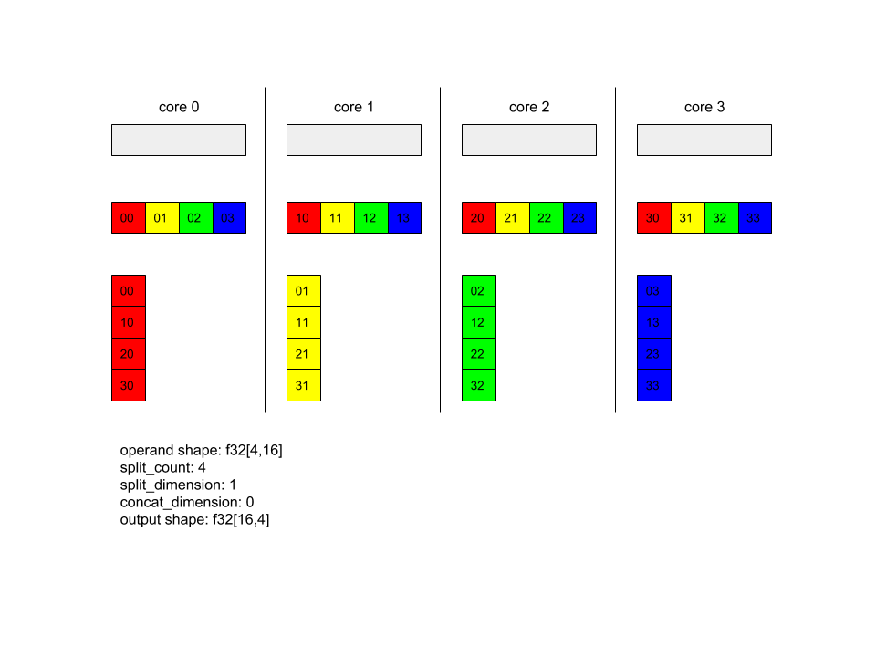
ในตัวอย่างนี้ มีแกน 4 แกนที่เข้าร่วมใน Alltoall ในแต่ละแกน ตัวถูกดำเนินการจะแบ่งออกเป็น 4 ส่วนตามมิติข้อมูล 0 ดังนั้นแต่ละส่วนจะมีรูปร่าง f32[4,4] ทั้ง 4 ส่วนกระจายอยู่ในแกนทั้งหมด จากนั้นแกนแต่ละแกนจะต่อส่วนที่ได้รับ ตามมิติข้อมูล 1 ตามลำดับของแกน 0-4 ดังนั้นเอาต์พุตในแต่ละแกน จะมีรูปร่าง f32[16,4]
BatchNormGrad
ดูคำอธิบายโดยละเอียดเกี่ยวกับอัลกอริทึมได้ที่
XlaBuilder::BatchNormGrad
และเอกสารการปรับรูปแบบมาตรฐานแบบกลุ่มฉบับเดิม
คำนวณการไล่ระดับสีของค่าฐานกลุ่ม
BatchNormGrad(operand, scale, mean, variance, grad_output, epsilon, feature_index)
| อาร์กิวเมนต์ | ประเภท | อรรถศาสตร์ |
|---|---|---|
operand |
XlaOp |
อาร์เรย์มิติ n ที่จะถูกทำให้เป็นมาตรฐาน (x) |
scale |
XlaOp |
อาร์เรย์มิติ 1 รายการ (\(\gamma\)) |
mean |
XlaOp |
อาร์เรย์มิติ 1 รายการ (\(\mu\)) |
variance |
XlaOp |
อาร์เรย์มิติ 1 รายการ (\(\sigma^2\)) |
grad_output |
XlaOp |
การไล่ระดับสีส่งผ่านไปยัง BatchNormTraining (\(\nabla y\)) |
epsilon |
float |
ค่า Epsilon (\(\epsilon\)) |
feature_index |
int64 |
ดัชนีสำหรับมิติข้อมูลจุดสนใจใน operand |
สำหรับแต่ละจุดสนใจในมิติข้อมูลของจุดสนใจ (feature_index คือดัชนีสำหรับมิติข้อมูลของจุดสนใจใน operand) การดำเนินการจะคำนวณการไล่ระดับสีด้วยอัตราส่วน operand, offset และ scale ในมิติข้อมูลอื่นๆ ทั้งหมด feature_index ต้องเป็นดัชนีที่ถูกต้องสำหรับมิติข้อมูลฟีเจอร์ใน operand
การไล่ระดับสี 3 แบบกำหนดด้วยสูตรต่อไปนี้ (สมมติว่าอาร์เรย์ 4 มิติเป็น operand และที่มีดัชนีมิติข้อมูลฟีเจอร์ l, ขนาดกลุ่ม m และขนาดเชิงพื้นที่ w และ h)
\[ \begin{split} c_l&= \frac{1}{mwh}\sum_{i=1}^m\sum_{j=1}^w\sum_{k=1}^h \left( \nabla y_{ijkl} \frac{x_{ijkl} - \mu_l}{\sigma^2_l+\epsilon} \right) \\\\ d_l&= \frac{1}{mwh}\sum_{i=1}^m\sum_{j=1}^w\sum_{k=1}^h \nabla y_{ijkl} \\\\ \nabla x_{ijkl} &= \frac{\gamma_{l} }{\sqrt{\sigma^2_{l}+\epsilon} } \left( \nabla y_{ijkl} - d_l - c_l (x_{ijkl} - \mu_{l}) \right) \\\\ \nabla \gamma_l &= \sum_{i=1}^m\sum_{j=1}^w\sum_{k=1}^h \left( \nabla y_{ijkl} \frac{x_{ijkl} - \mu_l}{\sqrt{\sigma^2_{l}+\epsilon} } \right) \\\\\ \nabla \beta_l &= \sum_{i=1}^m\sum_{j=1}^w\sum_{k=1}^h \nabla y_{ijkl} \end{split} \]
อินพุต mean และ variance แสดงถึงค่าช่วงเวลาในมิติข้อมูลแบบกลุ่มและมิติ
ประเภทเอาต์พุตจะเป็น Tuple ของแฮนเดิล 3 อัน ได้แก่
| เอาต์พุต | ประเภท | อรรถศาสตร์ |
|---|---|---|
grad_operand
|
XlaOp
|
การไล่ระดับสีตามอินพุต operand ($\nabla
x$) |
grad_scale
|
XlaOp
|
การไล่ระดับสีตามอินพุต scale ($\nabla
\gamma$) |
grad_offset
|
XlaOp
|
การไล่ระดับสีตามอินพุต offset($\nabla
\beta$) |
BatchNormInference
ดูคำอธิบายโดยละเอียดเกี่ยวกับอัลกอริทึมได้ที่
XlaBuilder::BatchNormInference
และเอกสารการปรับรูปแบบมาตรฐานแบบกลุ่มฉบับเดิม
ทำอาร์เรย์มาตรฐานตามกลุ่มมิติและมิติข้อมูลเชิงพื้นที่
BatchNormInference(operand, scale, offset, mean, variance, epsilon, feature_index)
| อาร์กิวเมนต์ | ประเภท | อรรถศาสตร์ |
|---|---|---|
operand |
XlaOp |
อาร์เรย์มิติ n ที่จะถูกทำให้เป็นมาตรฐาน |
scale |
XlaOp |
อาร์เรย์มิติข้อมูล 1 รายการ |
offset |
XlaOp |
อาร์เรย์มิติข้อมูล 1 รายการ |
mean |
XlaOp |
อาร์เรย์มิติข้อมูล 1 รายการ |
variance |
XlaOp |
อาร์เรย์มิติข้อมูล 1 รายการ |
epsilon |
float |
ค่า Epsilon |
feature_index |
int64 |
ดัชนีสำหรับมิติข้อมูลจุดสนใจใน operand |
สำหรับแต่ละจุดสนใจในมิติข้อมูลของจุดสนใจ (feature_index คือดัชนีสำหรับมิติข้อมูลของคุณลักษณะใน operand) การดำเนินการจะคำนวณค่าเฉลี่ยและความแปรปรวนในมิติข้อมูลอื่นๆ ทั้งหมด และใช้ค่าเฉลี่ยและความแปรปรวนเพื่อทำให้แต่ละองค์ประกอบใน operand เป็นมาตรฐาน feature_index ต้องเป็นดัชนีที่ถูกต้องสำหรับมิติข้อมูลฟีเจอร์ใน operand
BatchNormInference เทียบเท่ากับการเรียกใช้ BatchNormTraining โดยไม่ต้องคำนวณ mean และ variance สำหรับแต่ละกลุ่ม โดยใช้อินพุต mean และ variance แทนค่าโดยประมาณ วัตถุประสงค์ของการทดสอบนี้คือเพื่อลดเวลาในการตอบสนองในการอนุมาน จึงมีชื่อว่า BatchNormInference
เอาต์พุตคืออาร์เรย์มาตรฐาน n ที่มีรูปทรงเดียวกับอินพุต
operand
BatchNormTraining
ดูคำอธิบายโดยละเอียดของอัลกอริทึมได้ที่ XlaBuilder::BatchNormTraining และ the original batch normalization paper
ทำอาร์เรย์มาตรฐานตามกลุ่มมิติและมิติข้อมูลเชิงพื้นที่
BatchNormTraining(operand, scale, offset, epsilon, feature_index)
| อาร์กิวเมนต์ | ประเภท | อรรถศาสตร์ |
|---|---|---|
operand |
XlaOp |
อาร์เรย์มิติ n ที่จะถูกทำให้เป็นมาตรฐาน (x) |
scale |
XlaOp |
อาร์เรย์มิติ 1 รายการ (\(\gamma\)) |
offset |
XlaOp |
อาร์เรย์มิติ 1 รายการ (\(\beta\)) |
epsilon |
float |
ค่า Epsilon (\(\epsilon\)) |
feature_index |
int64 |
ดัชนีสำหรับมิติข้อมูลจุดสนใจใน operand |
สำหรับแต่ละจุดสนใจในมิติข้อมูลของจุดสนใจ (feature_index คือดัชนีสำหรับมิติข้อมูลของคุณลักษณะใน operand) การดำเนินการจะคำนวณค่าเฉลี่ยและความแปรปรวนในมิติข้อมูลอื่นๆ ทั้งหมด และใช้ค่าเฉลี่ยและความแปรปรวนเพื่อทำให้แต่ละองค์ประกอบใน operand เป็นมาตรฐาน feature_index ต้องเป็นดัชนีที่ถูกต้องสำหรับมิติข้อมูลฟีเจอร์ใน operand
อัลกอริทึมมีลักษณะดังต่อไปนี้สําหรับแต่ละกลุ่มใน operand \(x\) ที่มีองค์ประกอบ m ที่มี w และ h เป็นขนาดของมิติข้อมูลเชิงพื้นที่ (สมมติว่า operand เป็นอาร์เรย์ 4 มิติ)
คำนวณค่าเฉลี่ยแบบกลุ่ม \(\mu_l\) ของแต่ละฟีเจอร์
lในมิติข้อมูลฟีเจอร์: \(\mu_l=\frac{1}{mwh}\sum_{i=1}^m\sum_{j=1}^w\sum_{k=1}^h x_{ijkl}\)คำนวณความแปรปรวนของแบทช์ \(\sigma^2_l\): $\sigma^2l=\frac{1}{mwh}\sum{i=1}^m\sum{j=1}^w\sum{k=1}^h (x_{ijkl} - \mu_l)^2$
ทำให้เป็นมาตรฐาน ปรับขนาด และกะ: \(y_{ijkl}=\frac{\gamma_l(x_{ijkl}-\mu_l)}{\sqrt[2]{\sigma^2_l+\epsilon} }+\beta_l\)
โดยจะเพิ่มค่า epsilon เล็กน้อยเพื่อหลีกเลี่ยงข้อผิดพลาดการหารด้วย 0
ประเภทเอาต์พุตจะเป็น Tuple ของ XlaOp 3 รายการ:
| เอาต์พุต | ประเภท | อรรถศาสตร์ |
|---|---|---|
output
|
XlaOp
|
อาร์เรย์มิติ n ที่มีรูปทรงเดียวกับอินพุต
operand (y) |
batch_mean |
XlaOp |
อาร์เรย์มิติ 1 รายการ (\(\mu\)) |
batch_var |
XlaOp |
อาร์เรย์มิติ 1 รายการ (\(\sigma^2\)) |
batch_mean และ batch_var คือช่วงเวลาที่คำนวณจากมิติข้อมูลกลุ่มและมิติข้อมูลเชิงพื้นที่โดยใช้สูตรด้านบน
BitcastConvertType
ดู XlaBuilder::BitcastConvertType เพิ่มเติม
ดำเนินการบิตแคสต์ตามองค์ประกอบจากรูปร่างข้อมูลไปจนถึงรูปร่างเป้าหมาย เช่นเดียวกับ tf.bitcast ใน TensorFlow ขนาดอินพุตและเอาต์พุตต้องตรงกัน เช่น องค์ประกอบ s32 จะกลายเป็นองค์ประกอบ f32 ผ่านกิจวัตรบิตแคสต์ และองค์ประกอบ s32 1 รายการจะกลายเป็นองค์ประกอบ s8 4 รายการ มีการใช้ Bitcast ในแบบแคสต์ระดับต่ำ ดังนั้นเครื่องที่มีการแสดงจุดลอยตัวที่แตกต่างกันจะให้ผลลัพธ์ที่แตกต่างกัน
BitcastConvertType(operand, new_element_type)
| อาร์กิวเมนต์ | ประเภท | อรรถศาสตร์ |
|---|---|---|
operand |
XlaOp |
อาร์เรย์ประเภท T โดยมีความสว่าง D |
new_element_type |
PrimitiveType |
ประเภท U |
ขนาดของตัวถูกดำเนินการและรูปร่างเป้าหมายต้องตรงกัน นอกเหนือจากมิติข้อมูลสุดท้ายซึ่งจะเปลี่ยนแปลงตามอัตราส่วนของขนาดดั้งเดิมทั้งก่อนและหลังการแปลง
ประเภทองค์ประกอบต้นทางและปลายทางต้องไม่ใช่ Tuple
การแปลงบิตแคสต์เป็นประเภทพื้นฐานที่มีความกว้างต่างกัน
BitcastConvert คำสั่ง HLO รองรับกรณีที่ขนาดของประเภทองค์ประกอบเอาต์พุต T' ไม่เท่ากับขนาดขององค์ประกอบอินพุต T เนื่องจากการดำเนินการทั้งหมดเป็นแนวคิดของบิตแคสต์ และไม่ได้เปลี่ยนแปลงไบต์พื้นฐาน รูปร่างขององค์ประกอบเอาต์พุตจึงต้องเปลี่ยนแปลง สำหรับ B = sizeof(T), B' =
sizeof(T') มี 2 กรณีที่เป็นไปได้
อย่างแรก เมื่อ B > B' รูปร่างเอาต์พุตจะมีขนาดใหม่ที่เป็นขนาดย่อยมากที่สุด
B/B' เช่น
f16[10,2]{1,0} %output = f16[10,2]{1,0} bitcast-convert(f32[10]{0} %input)
กฎจะยังคงเหมือนเดิมสำหรับสเกลาร์ที่มีประสิทธิภาพ ดังนี้
f16[2]{0} %output = f16[2]{0} bitcast-convert(f32[] %input)
อีกทางเลือกหนึ่งสำหรับ B' > B วิธีการกำหนดให้มิติข้อมูลเชิงตรรกะสุดท้ายของรูปร่างอินพุตเท่ากับ B'/B และมิติข้อมูลนี้จะถูกตัดออกระหว่างการแปลง
f32[10]{0} %output = f32[10]{0} bitcast-convert(f16[10,2]{1,0} %input)
โปรดทราบว่าการแปลงระหว่างบิตกว้างที่แตกต่างกันไม่สามารถใช้ตามองค์ประกอบได้
ประกาศ
ดู XlaBuilder::Broadcast เพิ่มเติม
เพิ่มมิติข้อมูลลงในอาร์เรย์โดยการทำซ้ำข้อมูลในอาร์เรย์
Broadcast(operand, broadcast_sizes)
| อาร์กิวเมนต์ | ประเภท | อรรถศาสตร์ |
|---|---|---|
operand |
XlaOp |
อาร์เรย์ที่จะทำซ้ำ |
broadcast_sizes |
ArraySlice<int64> |
ขนาดของมิติข้อมูลใหม่ |
ระบบจะแทรกมิติข้อมูลใหม่ทางด้านซ้าย เช่น หาก broadcast_sizes มีค่า {a0, ..., aN} และรูปร่างตัวถูกดำเนินการมีขนาด {b0, ..., bM} รูปร่างของเอาต์พุตจะมีขนาด {a0, ..., aN, b0, ..., bM}
ระบบจะจัดทำดัชนีมิติข้อมูลใหม่ลงในสำเนาของตัวถูกดำเนินการ กล่าวคือ
output[i0, ..., iN, j0, ..., jM] = operand[j0, ..., jM]
เช่น หาก operand เป็นสเกลาร์ f32 ที่มีค่า 2.0f และ broadcast_sizes คือ {2, 3} ผลลัพธ์จะเป็นอาร์เรย์ที่มีรูปร่าง f32[2, 3] และค่าทั้งหมดในผลลัพธ์จะเป็น 2.0f
BroadcastInDim
ดู XlaBuilder::BroadcastInDim เพิ่มเติม
ขยายขนาดและอันดับของอาร์เรย์โดยการทำซ้ำข้อมูลในอาร์เรย์
BroadcastInDim(operand, out_dim_size, broadcast_dimensions)
| อาร์กิวเมนต์ | ประเภท | อรรถศาสตร์ |
|---|---|---|
operand |
XlaOp |
อาร์เรย์ที่จะทำซ้ำ |
out_dim_size |
ArraySlice<int64> |
ขนาดของรูปร่างเป้าหมาย |
broadcast_dimensions |
ArraySlice<int64> |
มิติข้อมูลใดในรูปร่างเป้าหมาย แต่ละมิติของรูปร่างตัวถูกดำเนินการสอดคล้องกับ |
คล้ายกับการออกอากาศ แต่อนุญาตให้เพิ่มมิติข้อมูลได้ทุกที่และขยายขนาดที่มีอยู่ด้วยขนาด 1
operand ออกอากาศเป็นรูปร่างที่อธิบายโดย out_dim_size
broadcast_dimensions จะจับคู่มิติข้อมูลของ operand กับขนาดของรูปร่างเป้าหมาย เช่น มิติข้อมูลที่ 1 ของตัวถูกดำเนินการแมปกับมิติข้อมูล broadcast_dimension[i] ของรูปร่างเอาต์พุต ขนาดของ operand ต้องมีขนาด 1 หรือเท่ากับขนาดในรูปร่างเอาต์พุตที่จับคู่กับมิติข้อมูลนั้น มิติข้อมูลที่เหลือจะแสดงด้วยขนาด 1 การออกอากาศมิติข้อมูลทำลายแล้วจะกระจายตามมิติข้อมูลที่เสื่อมลงเหล่านี้
เพื่อให้ได้รูปร่างเอาต์พุต ดูคำอธิบายความหมายอย่างละเอียดได้ในหน้าการออกอากาศ
โทร
ดู XlaBuilder::Call เพิ่มเติม
เรียกใช้การคํานวณด้วยอาร์กิวเมนต์ที่ระบุ
Call(computation, args...)
| อาร์กิวเมนต์ | ประเภท | อรรถศาสตร์ |
|---|---|---|
computation |
XlaComputation |
การคำนวณประเภท T_0, T_1, ..., T_{N-1} -> S ที่มีพารามิเตอร์ N ประเภทที่กำหนดเอง |
args |
ลำดับของ N XlaOp วินาที |
อาร์กิวเมนต์ N ประเภทที่กำหนดเอง |
อาร์กิวเมนต์และประเภทของ args ต้องตรงกับพารามิเตอร์ของ computation ไม่ได้รับอนุญาตให้ไม่มี args
โชเลสกี
ดู XlaBuilder::Cholesky เพิ่มเติม
คำนวณการแตกตัวของชูเลสกี้ของเมทริกซ์จำกัดค่าบวกแบบสมมาตร (เฮอร์มิเชียน)
Cholesky(a, lower)
| อาร์กิวเมนต์ | ประเภท | อรรถศาสตร์ |
|---|---|---|
a |
XlaOp |
อาร์เรย์อันดับ > 2 ของประเภทเชิงซ้อนหรือจุดลอยตัว |
lower |
bool |
จะใช้สามเหลี่ยมบนหรือล่างของ a |
หาก lower เป็น true จะคํานวณเมทริกซ์สามเหลี่ยมล่าง l ค่าที่ $a = l
l^T$ ถ้า lower เป็น false จะคํานวณเมทริกซ์บนสามเหลี่ยม u เท่ากับค่าดังกล่าว
\(a = u^T . u\)
ข้อมูลที่ป้อนจะอ่านจากสามเหลี่ยมล่าง/บนของ a เท่านั้น โดยขึ้นอยู่กับค่าของ lower และจะไม่สนใจค่าจากสามเหลี่ยมอื่นๆ ข้อมูลเอาต์พุตจะแสดงในสามเหลี่ยมเดียวกัน ค่าในสามเหลี่ยมอีกรูปหนึ่งเป็นตัวกำหนดการใช้งานและอาจเป็นอะไรก็ได้
หากอันดับของ a มากกว่า 2 จะถือว่า a เป็นชุดเมทริกซ์โดยที่ทั้งหมดยกเว้นมิติข้อมูลรอง 2 คือมิติข้อมูลกลุ่ม
หาก a ไม่ได้เป็นค่าบวกแบบสมมาตร (แบบเฮอร์มิเชียน) ผลลัพธ์จะเป็นค่าที่กำหนดจากการใช้งาน
แบบมีตัวหนีบ
ดู XlaBuilder::Clamp เพิ่มเติม
ยึดตัวถูกดำเนินการให้อยู่ในช่วงระหว่างค่าต่ำสุดและสูงสุด
Clamp(min, operand, max)
| อาร์กิวเมนต์ | ประเภท | อรรถศาสตร์ |
|---|---|---|
min |
XlaOp |
อาร์เรย์ประเภท T |
operand |
XlaOp |
อาร์เรย์ประเภท T |
max |
XlaOp |
อาร์เรย์ประเภท T |
จะแสดงผลตัวถูกดำเนินการหากอยู่ภายในช่วงระหว่างค่าต่ำสุดและสูงสุด แสดงผลค่าต่ำสุดหากตัวถูกดำเนินการต่ำกว่าช่วงนี้ หรือค่าสูงสุดหากตัวถูกดำเนินการอยู่เหนือช่วงนี้ ซึ่งก็คือ clamp(a, x, b) = min(max(a, x), b)
ทั้ง 3 อาร์เรย์ต้องมีรูปทรงเดียวกัน นอกจากนี้ รูปแบบที่จำกัดของ
การออกอากาศ, min และ/หรือ max อาจเป็นสเกลาร์ประเภท T
ตัวอย่างที่มีสเกลาร์ min และ max
let operand: s32[3] = {-1, 5, 9};
let min: s32 = 0;
let max: s32 = 6;
==>
Clamp(min, operand, max) = s32[3]{0, 5, 6};
ยุบ
โปรดดูเพิ่มเติมที่ XlaBuilder::Collapse และการดําเนินการ tf.reshape
ยุบมิติข้อมูลของอาร์เรย์เป็นมิติข้อมูลเดียว
Collapse(operand, dimensions)
| อาร์กิวเมนต์ | ประเภท | อรรถศาสตร์ |
|---|---|---|
operand |
XlaOp |
อาร์เรย์ประเภท T |
dimensions |
int64 เวกเตอร์ |
ส่วนย่อยของมิติข้อมูลของ T เรียงต่อกันตามลำดับ |
การยุบจะแทนที่ชุดย่อยของมิติข้อมูลของตัวถูกดำเนินการที่ระบุตามมิติข้อมูลเดียว อาร์กิวเมนต์อินพุตคืออาร์เรย์ประเภท T ที่กำหนดเองและเวกเตอร์คงที่เวลาคอมไพล์ของดัชนีมิติข้อมูล ดัชนีมิติข้อมูลต้องอยู่ในรูปแบบตามลำดับ (ตัวเลขมิติข้อมูลต่ำไปสูง) ชุดย่อยต่อเนื่องของมิติข้อมูล T ดังนั้น {0, 1, 2}, {0, 1} หรือ {1, 2} คือชุดมิติข้อมูลที่ถูกต้องทั้งหมด แต่ {1, 0} หรือ {0, 2} ไม่ใช่ มิติข้อมูลเหล่านี้จะถูกแทนที่ด้วยมิติข้อมูลใหม่ 1 มิติข้อมูล ในตำแหน่งเดียวกันในลำดับมิติข้อมูลกับมิติข้อมูลที่แทนที่ ที่มีขนาดมิติข้อมูลใหม่เท่ากับผลิตภัณฑ์ของขนาดมิติข้อมูลเดิม ตัวเลขมิติข้อมูลต่ำสุดใน dimensions คือมิติข้อมูลที่ช้าที่สุด (สำคัญที่สุด) ในวนซ้ำ Nest ซึ่งจะยุบมิติข้อมูลเหล่านี้ และจำนวนมิติข้อมูลสูงสุดคือต่างกันเร็วที่สุด (น้อยที่สุด) ดูโอเปอเรเตอร์ tf.reshape หากจำเป็นต้องใช้ลำดับการยุบทั่วไป
ตัวอย่างเช่น กำหนดให้ v เป็นอาร์เรย์ขององค์ประกอบ 24 รายการ
let v = f32[4x2x3] { { {10, 11, 12},  {15, 16, 17} },
{ {20, 21, 22},  {25, 26, 27} },
{ {30, 31, 32},  {35, 36, 37} },
{ {40, 41, 42},  {45, 46, 47} } };

// Collapse to a single dimension, leaving one dimension.
let v012 = Collapse(v, {0,1,2});
then v012 == f32[24] {10, 11, 12, 15, 16, 17,
20, 21, 22, 25, 26, 27,
30, 31, 32, 35, 36, 37,
40, 41, 42, 45, 46, 47};

// Collapse the two lower dimensions, leaving two dimensions.
let v01 = Collapse(v, {0,1});
then v01 == f32[4x6] { {10, 11, 12, 15, 16, 17},
{20, 21, 22, 25, 26, 27},
{30, 31, 32, 35, 36, 37},
{40, 41, 42, 45, 46, 47} };

// Collapse the two higher dimensions, leaving two dimensions.
let v12 = Collapse(v, {1,2});
then v12 == f32[8x3] { {10, 11, 12},
{15, 16, 17},
{20, 21, 22},
{25, 26, 27},
{30, 31, 32},
{35, 36, 37},
{40, 41, 42},
{45, 46, 47} };
CollectivePermute
ดู XlaBuilder::CollectivePermute เพิ่มเติม
CollectivePermute เป็นการดำเนินการร่วมกันที่ส่งและรับข้อมูลจากตัวจำลองที่หลากหลาย
CollectivePermute(operand, source_target_pairs)
| อาร์กิวเมนต์ | ประเภท | อรรถศาสตร์ |
|---|---|---|
operand |
XlaOp |
อาร์เรย์อินพุตมิติ n |
source_target_pairs |
<int64, int64> เวกเตอร์ |
รายการคู่ (source_replica_id, target_replica_id) สำหรับแต่ละคู่ ระบบจะส่งตัวถูกดำเนินการจากตัวจำลองต้นทางไปยังตัวจำลองเป้าหมาย |
โปรดทราบว่า source_target_pair มีข้อจำกัดดังต่อไปนี้
- ทั้ง 2 คู่ไม่ควรมีรหัสตัวจำลองเป้าหมายเดียวกัน และไม่ควรมีรหัสตัวจำลองต้นทางเดียวกัน
- หากรหัสการจำลองไม่ใช่เป้าหมายในคู่ใดๆ เอาต์พุตบนตัวจำลองนั้นจะเป็น tensor ที่ประกอบด้วย 0 ที่มีรูปทรงเดียวกับอินพุต
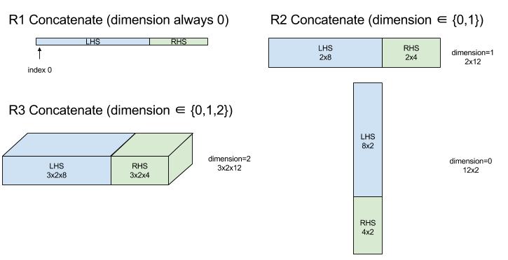
เชื่อมต่อ
ดู XlaBuilder::ConcatInDim เพิ่มเติม
การเชื่อมต่อจะเขียนอาร์เรย์จากตัวถูกดำเนินการอาร์เรย์หลายรายการ อาร์เรย์มีอันดับเดียวกันกับตัวถูกดำเนินการของอาร์เรย์อินพุตแต่ละรายการ (ซึ่งต้องอยู่ในอันดับเดียวกัน) และมีอาร์กิวเมนต์ตามลำดับที่ระบุไว้
Concatenate(operands..., dimension)
| อาร์กิวเมนต์ | ประเภท | อรรถศาสตร์ |
|---|---|---|
operands |
ลำดับของ N XlaOp |
N อาร์เรย์ประเภท T ที่มีขนาด [L0, L1, ...] ต้องการ N >= 1 |
dimension |
int64 |
ค่าในช่วง [0, N) ที่ตั้งชื่อมิติข้อมูลที่จะเชื่อมระหว่าง operands |
ยกเว้น dimension มิติข้อมูลทั้งหมดต้องเหมือนกัน เนื่องจาก XLA ไม่รองรับอาร์เรย์ที่ "ขรุขระ" และโปรดทราบว่าค่าอันดับ 0 จะเชื่อมโยงกันไม่ได้ (เนื่องจากไม่สามารถตั้งชื่อมิติข้อมูลที่มีการเชื่อมโยงเกิดขึ้น)
ตัวอย่าง 1 มิติ:
Concat({ {2, 3}, {4, 5}, {6, 7} }, 0)
>>> {2, 3, 4, 5, 6, 7}
ตัวอย่าง 2 มิติ:
let a = {
{1, 2},
{3, 4},
{5, 6},
};
let b = {
{7, 8},
};
Concat({a, b}, 0)
>>> {
{1, 2},
{3, 4},
{5, 6},
{7, 8},
}
แผนภาพ:
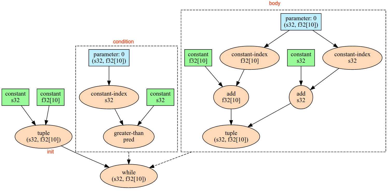
มีเงื่อนไข
ดู XlaBuilder::Conditional เพิ่มเติม
Conditional(pred, true_operand, true_computation, false_operand,
false_computation)
| อาร์กิวเมนต์ | ประเภท | อรรถศาสตร์ |
|---|---|---|
pred |
XlaOp |
สเกลของประเภท PRED |
true_operand |
XlaOp |
อาร์กิวเมนต์ของประเภท \(T_0\) |
true_computation |
XlaComputation |
XlaComputation ของประเภท \(T_0 \to S\) |
false_operand |
XlaOp |
อาร์กิวเมนต์ของประเภท \(T_1\) |
false_computation |
XlaComputation |
XlaComputation ของประเภท \(T_1 \to S\) |
เรียกใช้ true_computation หาก pred คือ true, false_computation หาก pred คือ false และแสดงผล
true_computation ต้องใช้อาร์กิวเมนต์ประเภทเดียว \(T_0\) และจะมีการเรียกใช้ด้วย true_operand ซึ่งต้องเป็นประเภทเดียวกัน false_computation ต้องใช้อาร์กิวเมนต์ประเภทเดียว \(T_1\) และจะเรียกใช้ด้วย false_operand ซึ่งต้องเป็นประเภทเดียวกัน ประเภทของค่าที่ส่งคืนของ true_computation และ false_computation ต้องเหมือนกัน
โปรดทราบว่าระบบจะเรียกใช้ true_computation และ false_computation เพียง 1 รายการเท่านั้น โดยขึ้นอยู่กับค่าของ pred
Conditional(branch_index, branch_computations, branch_operands)
| อาร์กิวเมนต์ | ประเภท | อรรถศาสตร์ |
|---|---|---|
branch_index |
XlaOp |
สเกลของประเภท S32 |
branch_computations |
ลำดับของ N XlaComputation |
XlaComputation ของประเภท \(T_0 \to S , T_1 \to S , ..., T_{N-1} \to S\) |
branch_operands |
ลำดับของ N XlaOp |
อาร์กิวเมนต์ของประเภท \(T_0 , T_1 , ..., T_{N-1}\) |
ดำเนินการ branch_computations[branch_index] และแสดงผลลัพธ์ หาก branch_index คือ S32 ซึ่ง < 0 หรือ >= N จะมีการเรียกใช้ branch_computations[N-1] เป็น Branch เริ่มต้น
branch_computations[b] แต่ละรายการต้องใช้อาร์กิวเมนต์ประเภทเดียว \(T_b\) และจะเรียกใช้ด้วย branch_operands[b] ซึ่งต้องเป็นประเภทเดียวกัน ประเภทของค่าที่ส่งคืนของ branch_computations[b] แต่ละรายการต้องเหมือนกัน
โปรดทราบว่าระบบจะดำเนินการ branch_computations เพียง 1 รายการเท่านั้น โดยขึ้นอยู่กับค่าของ branch_index
Conv. (คอนโวลูชัน)
ดู XlaBuilder::Conv เพิ่มเติม
เป็น ConvWithGeneralPadding แต่ระยะห่างจากขอบจะระบุแบบสั้นๆ เป็น SAME หรือ VALID ระยะห่างจากขอบเดียวกันจะใส่เลขศูนย์ให้กับอินพุต (lhs) เพื่อให้เอาต์พุตมีรูปร่างเดียวกันกับอินพุตเมื่อไม่ได้นับรวมไว้ด้วย ระยะห่างจากขอบที่ใช้ได้หมายถึงไม่มีระยะห่างจากขอบ
ConvWithGeneralPadding (การสนทนา)
ดู XlaBuilder::ConvWithGeneralPadding เพิ่มเติม
คำนวณคอนโวลูชันของชนิดที่ใช้ในโครงข่ายประสาท ในที่นี้ คอนโวลูชันอาจมองได้ว่าเป็นหน้าต่าง n มิติที่เคลื่อนผ่านพื้นที่ฐาน n และการคำนวณสำหรับแต่ละตำแหน่งที่เป็นไปได้ของหน้าต่าง
| อาร์กิวเมนต์ | ประเภท | อรรถศาสตร์ |
|---|---|---|
lhs |
XlaOp |
จัดอันดับอาร์เรย์ n+2 ของอินพุต |
rhs |
XlaOp |
แรงก์อันดับ n+2 ของน้ำหนักเคอร์เนล |
window_strides |
ArraySlice<int64> |
อาร์เรย์ n-d ของเคอร์เนล |
padding |
ArraySlice< pair<int64,int64>> |
อาร์เรย์ n-d ของระยะห่างจากขอบ (ต่ำ, สูง) |
lhs_dilation |
ArraySlice<int64> |
อาร์เรย์ตัวประกอบการขยาย lhs ของ n-d |
rhs_dilation |
ArraySlice<int64> |
อาร์เรย์ตัวประกอบการขยาย n-d rhs |
feature_group_count |
int64 | จำนวนกลุ่มฟีเจอร์ |
batch_group_count |
int64 | จํานวนกลุ่มของกลุ่ม |
กำหนดให้ n เป็นจำนวนของมิติข้อมูลเชิงพื้นที่ อาร์กิวเมนต์ lhs คืออาร์เรย์อันดับ n+2 ที่อธิบายพื้นที่ฐาน ซึ่งเรียกว่าอินพุต แม้ว่าแน่นอนว่า
rhs จะเป็นอินพุตก็ตาม ในโครงข่ายระบบประสาทเทียม อินพุตเหล่านี้คือการเปิดใช้งาน
มิติข้อมูล n+2 มีลําดับดังนี้
batch: แต่ละพิกัดในมิติข้อมูลนี้แสดงถึงอินพุตอิสระที่มีการดำเนินการคอนโวลูชันz/depth/features: แต่ละตำแหน่ง (y,x) ในพื้นที่ฐานจะมีเวกเตอร์เชื่อมโยงอยู่ ซึ่งจะอยู่ในมิติข้อมูลนี้spatial_dims: อธิบายมิติข้อมูลเชิงพื้นที่nที่กำหนดพื้นที่ฐานที่หน้าต่างเคลื่อนที่ข้าม
อาร์กิวเมนต์ rhs คืออาร์เรย์อันดับ n+2 ที่อธิบายตัวกรอง/เคอร์เนล/หน้าต่าง Convolutional มิติข้อมูลมีลําดับดังนี้
output-z: มิติข้อมูลzของเอาต์พุตinput-z: ขนาดของมิติข้อมูลนี้คูณfeature_group_countควรเท่ากับขนาดของมิติข้อมูลzในหน่วย lhsspatial_dims: อธิบายมิติข้อมูลเชิงพื้นที่nที่กำหนดหน้าต่าง n-d ที่เคลื่อนที่ผ่านพื้นที่ฐาน
อาร์กิวเมนต์ window_strides จะระบุอัตราเร็วของกรอบเวลาคอนโวลูชันในมิติข้อมูลเชิงพื้นที่ เช่น หากอัตราก้าวในมิติแรกคือ 3 เป้าหมายจะวางหน้าต่างที่พิกัดที่ดัชนีพิกัดแรกหารด้วย 3 ได้เท่านั้น
อาร์กิวเมนต์ padding จะระบุจำนวนระยะห่างจากขอบเป็น 0 ที่จะใช้กับพื้นที่ฐาน ระยะห่างจากขอบอาจเป็นค่าลบก็ได้ ค่าสัมบูรณ์ของระยะห่างจากขอบที่เป็นลบบ่งชี้ถึงจำนวนองค์ประกอบที่ต้องนำออกจากมิติข้อมูลที่ระบุก่อนทำคอนโวลูชัน padding[0] ระบุระยะห่างจากขอบสำหรับมิติข้อมูล y และ padding[1] จะระบุระยะห่างจากขอบของมิติข้อมูล x แต่ละคู่จะมีระยะห่างจากขอบต่ำเป็นองค์ประกอบแรก และมีระยะห่างจากขอบสูงเป็นองค์ประกอบที่สอง ระบบจะใช้ระยะห่างจากขอบต่ำในทิศทางของดัชนีด้านล่าง ส่วนระยะห่างจากขอบสูงจะใช้ในทิศทางของดัชนีที่สูงกว่า เช่น หาก padding[1] คือ (2,3) ก็จะมีระยะห่างจากขอบ 2 จุดทางด้านซ้าย และ 0 3 ตัวทางด้านขวาในมิติข้อมูลเชิงพื้นที่ที่ 2 การใช้ระยะห่างจากขอบเทียบเท่ากับการแทรกค่าที่เป็น 0 เดียวกันเหล่านั้นลงในอินพุต (lhs) ก่อนที่จะทำ Conversion
อาร์กิวเมนต์ lhs_dilation และ rhs_dilation จะระบุปัจจัยการขยายที่จะใช้กับ lhs และ rhs ตามลำดับในมิติมิติของแต่ละมิติ หากปัจจัยการขยายในมิติข้อมูลเชิงพื้นที่คือ d ระบบจะวางหลุม d-1 ระหว่างแต่ละรายการในมิติข้อมูลนั้นโดยปริยาย ซึ่งจะเพิ่มขนาดของอาร์เรย์ ค่าที่ไม่มีการดำเนินการในหลุมจะเต็ม ซึ่งคำว่าคอนโวลูชันหมายถึงค่าซีโร
การขยายตัวของ RHS เรียกอีกอย่างว่า Atrous Convolution ดูรายละเอียดเพิ่มเติมได้ที่ tf.nn.atrous_conv2d การขยาย lhs เรียกอีกอย่างหนึ่งว่าคอนโวลูชันสลับตำแหน่ง (Transposed Convolution) ดูรายละเอียดเพิ่มเติมได้ที่ tf.nn.conv2d_transpose
คุณใช้อาร์กิวเมนต์ feature_group_count (ค่าเริ่มต้น 1) สำหรับ Conversion แบบกลุ่มได้ feature_group_count ต้องเป็นตัวหารของทั้งมิติข้อมูลฟีเจอร์อินพุตและเอาต์พุต หาก feature_group_count มากกว่า 1 หมายความว่าในเชิงมโนทัศน์ว่ามิติข้อมูลฟีเจอร์อินพุตและเอาต์พุตและมิติข้อมูลฟีเจอร์เอาต์พุต rhs จะแบ่งออกเป็นกลุ่ม feature_group_count หลายกลุ่มเท่าๆ กัน โดยแต่ละกลุ่มประกอบด้วยชุดฟีเจอร์ต่อกัน มิติข้อมูลฟีเจอร์อินพุตของ rhs ต้องเท่ากับมิติข้อมูลฟีเจอร์อินพุต lhs หารด้วย feature_group_count (จึงมีขนาดกลุ่มฟีเจอร์อินพุตอยู่แล้ว) ระบบจะใช้กลุ่มที่ i ร่วมกันเพื่อคำนวณ feature_group_count สำหรับคอนโวลูชันที่แยกกันหลายรายการ ผลลัพธ์ของ Conversion เหล่านี้จะต่อเข้าด้วยกันในมิติข้อมูลของฟีเจอร์เอาต์พุต
สำหรับ Convolution แบบ Insights ระบบจะตั้งค่าอาร์กิวเมนต์ feature_group_count เป็นมิติข้อมูลฟีเจอร์อินพุต และจะเปลี่ยนรูปร่างตัวกรองจาก [filter_height, filter_width, in_channels, channel_multiplier] เป็น [filter_height, filter_width, 1, in_channels * channel_multiplier] ดูรายละเอียดเพิ่มเติมได้ที่ tf.nn.depthwise_conv2d
คุณใช้อาร์กิวเมนต์ batch_group_count (ค่าเริ่มต้น 1) กับตัวกรองที่จัดกลุ่มได้ระหว่างการนำไปใช้งานหลังการ batch_group_count ต้องเป็นตัวหารของมิติข้อมูลกลุ่ม lhs (อินพุต) หาก batch_group_count มากกว่า 1 หมายความว่ามิติข้อมูลกลุ่มเอาต์พุตควรมีขนาด input batch
/ batch_group_count batch_group_count ต้องเป็นตัวหารของขนาดฟีเจอร์เอาต์พุต
รูปร่างเอาต์พุตมีขนาดดังต่อไปนี้
batch: ขนาดของมิติข้อมูลนี้คูณbatch_group_countควรเท่ากับขนาดของมิติข้อมูลbatchในหน่วย lhsz: ขนาดเท่ากับoutput-zบนเคอร์เนล (rhs)spatial_dims: ค่า 1 ค่าสำหรับตำแหน่งกรอบเวลาคอนโวลูชันที่ถูกต้องแต่ละตำแหน่ง

รูปด้านบนแสดงวิธีการทำงานของฟิลด์ batch_group_count อย่างมีประสิทธิภาพ เราจะแบ่งแต่ละหลักออกเป็น batch_group_count กลุ่ม และทำแบบเดียวกันนี้สำหรับฟีเจอร์เอาต์พุต จากนั้นเราจะจับคู่แบบ 2 กลุ่มและเชื่อมโยงเอาต์พุตตามมิติข้อมูลของฟีเจอร์เอาต์พุตสำหรับแต่ละกลุ่ม ความหมายในการดำเนินการของมิติข้อมูลอื่นๆ ทั้งหมด (ฟีเจอร์และเชิงพื้นที่) จะยังคงเหมือนเดิม
ตำแหน่งที่ถูกต้องของกรอบเวลาคอนโวลูชันจะกำหนดโดยจังหวะก้าวและขนาดของพื้นที่ฐานหลังระยะห่างจากขอบ
หากต้องการอธิบายหน้าที่ของคอนโวลูชัน ให้พิจารณาคอนโวลูชัน 2 มิติและเลือกพิกัด batch, z, y, x คงที่ในเอาต์พุต แล้ว (y,x) จะเป็นตำแหน่งมุมของหน้าต่างภายในพื้นที่ฐาน (เช่น มุมซ้ายบน ขึ้นอยู่กับวิธีที่คุณตีความมิติข้อมูลเชิงพื้นที่) ตอนนี้เรามีหน้าต่าง 2 มิติ
ที่ถ่ายจากพื้นที่ฐาน ซึ่งจุด 2 มิติแต่ละจุดเชื่อมโยงกับเวกเตอร์ 1 มิติ
เราจึงได้กล่อง 3 มิติ จากเคอร์เนล Convolutional นับตั้งแต่ที่เราแก้ไขพิกัดเอาต์พุต z เรายังมีกล่อง 3 มิติด้วย กล่อง 2 กล่องนี้มีขนาดเท่ากัน เราจึงหาผลรวมของผลลัพธ์ตามองค์ประกอบระหว่าง 2 กล่องได้ (คล้ายกับผลิตภัณฑ์จุด) นั่นคือค่าเอาต์พุต
โปรดทราบว่าหากใช้ output-z เช่น 5 จากนั้นแต่ละตำแหน่งของหน้าต่างจะสร้างค่า 5 ค่าในเอาต์พุตไปยังมิติข้อมูล z ของเอาต์พุตนั้น ค่าเหล่านี้จะแตกต่างกันไปในส่วนที่ใช้ส่วนของเคอร์เนล Convolutional เพราะมีกล่อง 3 มิติที่แยกค่าไว้ใช้สำหรับ output-z แต่ละพิกัด เปรียบได้กับ Conversion 5 แบบ
โดยมีตัวกรองที่ต่างกันสำหรับแต่ละกลุ่ม
นี่คือรหัสเทียมสำหรับคอนโวลูชัน 2 มิติที่มีระยะห่างจากขอบและขั้น
for (b, oz, oy, ox) {  // output coordinates
  value = 0;
  for (iz, ky, kx) {  // kernel coordinates and input z
    iy = oy*stride_y + ky - pad_low_y;
    ix = ox*stride_x + kx - pad_low_x;
    if ((iy, ix) inside the base area considered without padding) {
      value += input(b, iz, iy, ix) * kernel(oz, iz, ky, kx);
    }
  }
  output(b, oz, oy, ox) = value;
}
ConvertElementType
ดู XlaBuilder::ConvertElementType เพิ่มเติม
การดำเนินการ Conversion ตามองค์ประกอบจากรูปร่างข้อมูลเป็นรูปร่างเป้าหมาย คล้ายกับ static_cast ตามองค์ประกอบใน C++ มิติข้อมูลต้องตรงกัน และ Conversion เป็นไปตามองค์ประกอบที่ต้องการ เช่น องค์ประกอบ s32 กลายเป็นองค์ประกอบ f32 ผ่านกิจวัตร Conversion s32 เป็น f32
ConvertElementType(operand, new_element_type)
| อาร์กิวเมนต์ | ประเภท | อรรถศาสตร์ |
|---|---|---|
operand |
XlaOp |
อาร์เรย์ประเภท T โดยมีความสว่าง D |
new_element_type |
PrimitiveType |
ประเภท U |
ขนาดของตัวถูกดำเนินการและรูปร่างเป้าหมายต้องตรงกัน ประเภทองค์ประกอบต้นทางและปลายทางต้องไม่ใช่ Tuple
Conversion อย่าง T=s32 เป็น U=f32 จะทำกิจวัตร Conversion แบบ int-to-Float ให้เป็นมาตรฐาน เช่น ปัดเศษไปใกล้ที่สุด
let a: s32[3] = {0, 1, 2};
let b: f32[3] = convert(a, f32);
then b == f32[3]{0.0, 1.0, 2.0}
CrossReplicaSum
ดำเนินการ AllReduce ที่มีการคำนวณผลรวม
CustomCall
ดู XlaBuilder::CustomCall เพิ่มเติม
เรียกใช้ฟังก์ชันที่ผู้ใช้ให้ไว้ภายในการคํานวณ
CustomCall(target_name, args..., shape)
| อาร์กิวเมนต์ | ประเภท | อรรถศาสตร์ |
|---|---|---|
target_name |
string |
ชื่อของฟังก์ชัน คำสั่งในการเรียกจะแสดงซึ่งจะกำหนดเป้าหมายไปยังชื่อสัญลักษณ์นี้ |
args |
ลำดับของ N XlaOp วินาที |
อาร์กิวเมนต์ N ประเภทที่กำหนดเอง ซึ่งจะส่งไปยังฟังก์ชัน |
shape |
Shape |
รูปร่างเอาต์พุตของฟังก์ชัน |
ลายเซ็นของฟังก์ชันจะเหมือนกัน โดยไม่คำนึงถึง Arity หรืออาร์กิวเมนต์ประเภทใดก็ตาม ดังนี้
extern "C" void target_name(void* out, void** in);
ตัวอย่างเช่น หากใช้ CustomCall ดังนี้
let x = f32[2] {1,2};
let y = f32[2x3] { {10, 20, 30}, {40, 50, 60} };

CustomCall("myfunc", {x, y}, f32[3x3])
ตัวอย่างการใช้งาน myfunc
extern "C" void myfunc(void* out, void** in) {
  float (&x)[2] = *static_cast<float(*)[2]>(in[0]);
  float (&y)[2][3] = *static_cast<float(*)[2][3]>(in[1]);
  EXPECT_EQ(1, x[0]);
  EXPECT_EQ(2, x[1]);
  EXPECT_EQ(10, y[0][0]);
  EXPECT_EQ(20, y[0][1]);
  EXPECT_EQ(30, y[0][2]);
  EXPECT_EQ(40, y[1][0]);
  EXPECT_EQ(50, y[1][1]);
  EXPECT_EQ(60, y[1][2]);
  float (&z)[3][3] = *static_cast<float(*)[3][3]>(out);
  z[0][0] = x[1] + y[1][0];
  // ...
}
ฟังก์ชันที่ได้จากผู้ใช้ต้องไม่มีผลข้างเคียงและการดําเนินการต้องเท่ากับ
จุด
ดู XlaBuilder::Dot เพิ่มเติม
Dot(lhs, rhs)
| อาร์กิวเมนต์ | ประเภท | อรรถศาสตร์ |
|---|---|---|
lhs |
XlaOp |
อาร์เรย์ประเภท T |
rhs |
XlaOp |
อาร์เรย์ประเภท T |
ความหมายที่แน่นอนของการดำเนินการนี้ขึ้นอยู่กับอันดับของตัวถูกดำเนินการ
| อินพุต | เอาต์พุต | อรรถศาสตร์ |
|---|---|---|
เวกเตอร์ [n] dot เวกเตอร์ [n] |
สเกลาร์ | ผลิตภัณฑ์เวกเตอร์จุด |
เมทริกซ์ [m x k] dot เวกเตอร์ [k] |
เวกเตอร์ [m] | การคูณเวกเตอร์เมทริกซ์ |
เมทริกซ์ [m x k] dot เมทริกซ์ [k x n] |
เมทริกซ์ [m x n] | การคูณเมทริกซ์เมทริกซ์ |
การดำเนินการนี้จะดำเนินการรวมผลิตภัณฑ์เกินมิติข้อมูลที่ 2 ของ lhs (หรือมิติข้อมูลแรกหากมีอันดับ 1) และมิติข้อมูลที่ 1 เป็น rhs ซึ่งก็คือมิติข้อมูล
"สัญญา" ขนาดตามสัญญาของ lhs และ rhs ต้องมีขนาดเท่ากัน ในทางปฏิบัติ สามารถใช้ในเรื่องการคูณจุดระหว่างเวกเตอร์ การคูณเวกเตอร์/เมทริกซ์ หรือการคูณเมทริกซ์/เมทริกซ์
DotGeneral
ดู XlaBuilder::DotGeneral เพิ่มเติม
DotGeneral(lhs, rhs, dimension_numbers)
| อาร์กิวเมนต์ | ประเภท | อรรถศาสตร์ |
|---|---|---|
lhs |
XlaOp |
อาร์เรย์ประเภท T |
rhs |
XlaOp |
อาร์เรย์ประเภท T |
dimension_numbers |
DotDimensionNumbers |
หมายเลขมิติข้อมูลการทำสัญญาและแบบกลุ่ม |
คล้ายกับจุด แต่อนุญาตให้ระบุหมายเลขมิติข้อมูลการทำสัญญาและแบบกลุ่มสำหรับทั้ง lhs และ rhs
| ช่อง DotDimensionNumbers | ประเภท | อรรถศาสตร์ |
|---|---|---|
lhs_contracting_dimensions
|
int64 ซ้ำ | หมายเลขมิติข้อมูลการทำสัญญา lhs รายการ |
rhs_contracting_dimensions
|
int64 ซ้ำ | หมายเลขมิติข้อมูลการทำสัญญา rhs รายการ |
lhs_batch_dimensions
|
int64 ซ้ำ | หมายเลขมิติข้อมูล
กลุ่ม lhs รายการ |
rhs_batch_dimensions
|
int64 ซ้ำ | หมายเลขมิติข้อมูล
กลุ่ม rhs รายการ |
DotGeneral ดำเนินการรวมผลิตภัณฑ์ผ่านมิติข้อมูลการทำสัญญาที่ระบุไว้ใน dimension_numbers
หมายเลขมิติข้อมูลการทำสัญญาที่เชื่อมโยงจาก lhs และ rhs ไม่จำเป็นต้องเหมือนกัน แต่ต้องมีขนาดมิติข้อมูลเท่ากัน
ตัวอย่างหมายเลขมิติข้อมูลการทำสัญญา
lhs = { {1.0, 2.0, 3.0},
{4.0, 5.0, 6.0} }

rhs = { {1.0, 1.0, 1.0},
{2.0, 2.0, 2.0} }

DotDimensionNumbers dnums;
dnums.add_lhs_contracting_dimensions(1);
dnums.add_rhs_contracting_dimensions(1);

DotGeneral(lhs, rhs, dnums) -> { {6.0, 12.0},
{15.0, 30.0} }
หมายเลขมิติข้อมูลกลุ่มที่เชื่อมโยงจาก lhs และ rhs จะต้องมีขนาดมิติข้อมูลเท่ากัน
ตัวอย่างที่มีหมายเลขมิติข้อมูลกลุ่ม (ขนาดกลุ่ม 2, เมทริกซ์ 2x2):
lhs = { { {1.0, 2.0},
{3.0, 4.0} },
{ {5.0, 6.0},
{7.0, 8.0} } }

rhs = { { {1.0, 0.0},
{0.0, 1.0} },
{ {1.0, 0.0},
{0.0, 1.0} } }

DotDimensionNumbers dnums;
dnums.add_lhs_contracting_dimensions(2);
dnums.add_rhs_contracting_dimensions(1);
dnums.add_lhs_batch_dimensions(0);
dnums.add_rhs_batch_dimensions(0);

DotGeneral(lhs, rhs, dnums) -> { { {1.0, 2.0},
{3.0, 4.0} },
{ {5.0, 6.0},
{7.0, 8.0} } }
| อินพุต | เอาต์พุต | อรรถศาสตร์ |
|---|---|---|
[b0, m, k] dot [b0, k, n] |
[b0, m, n] | แบตต์มัล |
[b0, b1, m, k] dot [b0, b1, k, n] |
[b0, b1, m, n] | แบตต์มัล |
ซึ่งหลังจากที่หมายเลขมิติข้อมูลที่ได้ขึ้นต้นด้วยมิติข้อมูลกลุ่ม จากนั้นเป็นมิติข้อมูลแบบไม่ทำสัญญา/ไม่ใช่กลุ่ม lhs และสุดท้ายคือมิติข้อมูล rhs ที่ไม่ทำสัญญา/ไม่ใช่กลุ่ม
DynamicSlice
ดู XlaBuilder::DynamicSlice เพิ่มเติม
DynamicSlice แยกอาร์เรย์ย่อยจากอาร์เรย์อินพุตที่ start_indices แบบไดนามิก ระบบจะส่งขนาดของชิ้นส่วนในแต่ละมิติข้อมูลใน size_indices ซึ่งระบุจุดสิ้นสุดของช่วงส่วนแบ่งพิเศษในแต่ละมิติข้อมูล: [เริ่มต้น, เริ่มต้น + ขนาด) รูปร่างของ start_indices ต้องมีอันดับ ==
1 โดยมีขนาดมิติข้อมูลเท่ากับอันดับของ operand
DynamicSlice(operand, start_indices, size_indices)
| อาร์กิวเมนต์ | ประเภท | อรรถศาสตร์ |
|---|---|---|
operand |
XlaOp |
อาร์เรย์มิติ N ของประเภท T |
start_indices |
ลำดับของ N XlaOp |
รายการจำนวนเต็มสเกลาร์ N ที่มีดัชนีเริ่มต้นของสไลซ์สำหรับแต่ละมิติข้อมูล ค่าต้องมากกว่าหรือเท่ากับ 0 |
size_indices |
ArraySlice<int64> |
รายการจำนวนเต็ม N ที่มีขนาดของสไลซ์สำหรับแต่ละมิติข้อมูล ค่าแต่ละค่าต้องมากกว่า 0 เท่านั้น และเริ่มต้น + ขนาดต้องน้อยกว่าหรือเท่ากับขนาดของมิติข้อมูลเพื่อหลีกเลี่ยงการตัดขนาดมิติข้อมูลโมดูล |
ดัชนีส่วนแบ่งที่มีประสิทธิภาพจะคำนวณโดยใช้การเปลี่ยนรูปแบบต่อไปนี้สำหรับดัชนี i แต่ละรายการใน [1, N) ก่อนดำเนินการสไลซ์
start_indices[i] = clamp(start_indices[i], 0, operand.dimension_size[i] - size_indices[i])
วิธีนี้ช่วยให้มั่นใจว่าสไลซ์ที่ดึงข้อมูลจะอยู่ในขอบเขตที่เกี่ยวข้องกับอาร์เรย์ตัวถูกดำเนินการเสมอ หากสไลซ์อยู่ในขอบเขตก่อนที่จะใช้การเปลี่ยนรูปแบบ การเปลี่ยนรูปแบบจะไม่มีผล
ตัวอย่าง 1 มิติ:
let a = {0.0, 1.0, 2.0, 3.0, 4.0}
let s = {2}

DynamicSlice(a, s, {2}) produces:
{2.0, 3.0}
ตัวอย่าง 2 มิติ:
let b =
{ {0.0,  1.0,  2.0},
{3.0,  4.0,  5.0},
{6.0,  7.0,  8.0},
{9.0, 10.0, 11.0} }
let s = {2, 1}

DynamicSlice(b, s, {2, 2}) produces:
{ { 7.0,  8.0},
{10.0, 11.0} }
DynamicUpdateSlice
ดู XlaBuilder::DynamicUpdateSlice เพิ่มเติม
DynamicUpdateSlice จะสร้างผลลัพธ์ซึ่งเป็นค่าของอาร์เรย์อินพุต operand โดยเขียนทับชิ้นส่วน update ที่ start_indices
รูปร่างของ update จะกำหนดรูปร่างของอาร์เรย์ย่อยของผลลัพธ์ที่มีการอัปเดต
รูปร่างของ start_indices ต้องมีอันดับ == 1 โดยมีขนาดมิติข้อมูลเท่ากับอันดับของ operand
DynamicUpdateSlice(operand, update, start_indices)
| อาร์กิวเมนต์ | ประเภท | อรรถศาสตร์ |
|---|---|---|
operand |
XlaOp |
อาร์เรย์มิติ N ของประเภท T |
update |
XlaOp |
N อาร์เรย์มิติของประเภท T ที่มีการอัปเดตส่วนแบ่ง มิติข้อมูลแต่ละรายการของรูปร่างการอัปเดตจะต้องมีค่ามากกว่า 0 และการเริ่มต้น + อัปเดตต้องน้อยกว่าหรือเท่ากับขนาดตัวถูกดำเนินการสำหรับแต่ละมิติข้อมูลเพื่อหลีกเลี่ยงการสร้างดัชนีการอัปเดตที่อยู่นอกขอบเขต |
start_indices |
ลำดับของ N XlaOp |
รายการจำนวนเต็มสเกลาร์ N ที่มีดัชนีเริ่มต้นของสไลซ์สำหรับแต่ละมิติข้อมูล ค่าต้องมากกว่าหรือเท่ากับ 0 |
ดัชนีส่วนแบ่งที่มีประสิทธิภาพจะคำนวณโดยใช้การเปลี่ยนรูปแบบต่อไปนี้สำหรับดัชนี i แต่ละรายการใน [1, N) ก่อนดำเนินการสไลซ์
start_indices[i] = clamp(start_indices[i], 0, operand.dimension_size[i] - update.dimension_size[i])
วิธีนี้ช่วยให้มั่นใจว่าส่วนแบ่งที่อัปเดตจะอยู่ในขอบเขตที่เกี่ยวข้องกับอาร์เรย์ตัวถูกดำเนินการเสมอ หากสไลซ์อยู่ในขอบเขตก่อนที่จะใช้การเปลี่ยนรูปแบบ การเปลี่ยนรูปแบบจะไม่มีผล
ตัวอย่าง 1 มิติ:
let a = {0.0, 1.0, 2.0, 3.0, 4.0}
let u = {5.0, 6.0}
let s = {2}

DynamicUpdateSlice(a, u, s) produces:
{0.0, 1.0, 5.0, 6.0, 4.0}
ตัวอย่าง 2 มิติ:
let b =
{ {0.0,  1.0,  2.0},
{3.0,  4.0,  5.0},
{6.0,  7.0,  8.0},
{9.0, 10.0, 11.0} }
let u =
{ {12.0,  13.0},
{14.0,  15.0},
{16.0,  17.0} }

let s = {1, 1}

DynamicUpdateSlice(b, u, s) produces:
{ {0.0,  1.0,  2.0},
{3.0, 12.0, 13.0},
{6.0, 14.0, 15.0},
{9.0, 16.0, 17.0} }
การดำเนินการทางเลขฐานสองตามองค์ประกอบ
ดู XlaBuilder::Add เพิ่มเติม
ระบบรองรับชุดการดำเนินการเลขฐานสองแบบ Element-wise
Op(lhs, rhs)
โดยที่ Op เป็นหนึ่งใน Add (การเพิ่ม) Sub (การลบ) Mul (การคูณ), Div (การหาร), Rem (ที่เหลืออยู่), Max (สูงสุด), Min
(ต่ำสุด), LogicalAnd (ตรรกะ AND) หรือ LogicalOr (ตรรกะ OR)
| อาร์กิวเมนต์ | ประเภท | อรรถศาสตร์ |
|---|---|---|
lhs |
XlaOp |
ตัวถูกดำเนินการด้านซ้าย: อาร์เรย์ของประเภท T |
rhs |
XlaOp |
ตัวถูกดำเนินการด้านขวา: อาร์เรย์ของประเภท T |
รูปร่างของอาร์กิวเมนต์ต้องคล้ายกันหรือใช้ร่วมกันได้ ดูเอกสารประกอบของการเผยแพร่เกี่ยวกับความหมายของรูปร่างที่เข้ากันได้ ผลที่ได้ของการดำเนินการจะมีรูปร่างซึ่งเป็นผลลัพธ์ของการเผยแพร่อาร์เรย์อินพุต 2 รายการ ในตัวแปรนี้ ระบบจะไม่รองรับการดำเนินการระหว่างอาร์เรย์ที่มีอันดับต่างกัน เว้นแต่ตัวถูกดำเนินการตัวใดตัวหนึ่งเป็นสเกลาร์
เมื่อ Op เท่ากับ Rem เครื่องหมายของผลลัพธ์จะนำมาจากตัวตั้งหาร และค่าสัมบูรณ์ของผลลัพธ์จะน้อยกว่าค่าสัมบูรณ์ของตัวหาร
ส่วนเกินของการหารจำนวนเต็ม (การหาร/ไม่มีการลงชื่อ/คงเหลือโดย 0 หรือหาร/จำนวนที่เหลือของ INT_SMIN ที่มี -1) จะสร้างค่าที่กำหนดการใช้งาน
มีตัวแปรอื่นที่รองรับการออกอากาศในระดับต่างกันสำหรับการดำเนินการต่อไปนี้
Op(lhs, rhs, broadcast_dimensions)
โดย Op เหมือนกับด้านบน ควรใช้ตัวแปรนี้สำหรับการดำเนินการทางคณิตศาสตร์ระหว่างอาร์เรย์ของอันดับที่ต่างกัน (เช่น การเพิ่มเมทริกซ์ให้กับเวกเตอร์)
ตัวถูกดำเนินการ broadcast_dimensions ที่เพิ่มเข้ามาคือส่วนของจำนวนเต็มที่ใช้เพื่อขยายอันดับของตัวถูกดำเนินการอันดับต่ำนั้นจนถึงอันดับของโอเปอแรนด์อันดับที่สูงกว่า broadcast_dimensions จะแมปมิติข้อมูลของรูปร่างอันดับต่ำกับมิติข้อมูลของรูปร่างอันดับสูงกว่า รูปร่างที่ขยายแล้วจะไม่จำกัดขนาดของ
รูปร่างที่ขยายแล้วจะแสดงด้วยขนาดที่ 1 การออกอากาศมิติข้อมูลที่เสื่อมสภาพแล้วจะเผยแพร่รูปร่างตามมิติข้อมูลที่เสื่อมลงเหล่านี้ เพื่อให้รูปร่างของตัวถูกดำเนินการทั้งคู่เท่ากัน ดูคำอธิบายความหมายอย่างละเอียดได้ในหน้าการออกอากาศ
การดำเนินการเปรียบเทียบตามองค์ประกอบ
ดู XlaBuilder::Eq เพิ่มเติม
ระบบรองรับชุดการดำเนินการเปรียบเทียบไบนารีตามองค์ประกอบมาตรฐาน โปรดทราบว่าจะมีการใช้ความหมายของการเปรียบเทียบจุดลอยตัว IEEE 754 แบบมาตรฐานเมื่อเปรียบเทียบประเภทจุดลอยตัว
Op(lhs, rhs)
โดยที่ Op เป็นหนึ่งใน Eq (เท่ากับ), Ne (ไม่เท่ากับ), Ge
(มากกว่าหรือเท่ากัน), Gt (มากกว่า), Le (น้อยกว่าหรือเท่ากับ) Lt
(น้อยกว่า) โอเปอเรเตอร์อีกชุดหนึ่ง คือ EqTotalOrder, NeTotalOrder, GeTotalOrder, GtTotalOrder, LeTotalOrder และ LtTotalOrder แล้ว ชุดการทำงานที่เหมือนกัน
เว้นแต่ชุดตัวนี้จะรองรับลำดับทั้งหมดเหนือจำนวนจุดลอยตัว โดยบังคับใช้ -NaN < -Inf < -Finite < -0 < f0 < +Finite
| อาร์กิวเมนต์ | ประเภท | อรรถศาสตร์ |
|---|---|---|
lhs |
XlaOp |
ตัวถูกดำเนินการด้านซ้าย: อาร์เรย์ของประเภท T |
rhs |
XlaOp |
ตัวถูกดำเนินการด้านขวา: อาร์เรย์ของประเภท T |
รูปร่างของอาร์กิวเมนต์ต้องคล้ายกันหรือใช้ร่วมกันได้ ดูเอกสารประกอบของการเผยแพร่เกี่ยวกับความหมายของรูปร่างที่เข้ากันได้ ผลที่ได้ของการดำเนินการจะมีรูปร่างซึ่งเป็นผลลัพธ์ของการเผยแพร่อาร์เรย์อินพุต 2 รายการที่มีประเภทองค์ประกอบ PRED ในตัวแปรนี้ ระบบจะไม่รองรับการดำเนินการระหว่างอาร์เรย์ที่มีอันดับต่างๆ กัน เว้นแต่ตัวถูกดำเนินการตัวใดตัวหนึ่งเป็นสเกลาร์
มีตัวแปรอื่นที่รองรับการออกอากาศในระดับต่างกันสำหรับการดำเนินการต่อไปนี้
Op(lhs, rhs, broadcast_dimensions)
โดย Op เหมือนกับด้านบน ควรใช้ตัวแปรของการดำเนินการนี้สำหรับการดำเนินการเปรียบเทียบระหว่างอาร์เรย์ของอันดับที่ต่างกัน (เช่น การเพิ่มเมทริกซ์ให้กับเวกเตอร์)
ตัวถูกดำเนินการ broadcast_dimensions เพิ่มเติมคือส่วนแบ่งของจำนวนเต็มที่ระบุมิติข้อมูลที่จะใช้สำหรับการกระจายตัวถูกดำเนินการ ดูคำอธิบายความหมายอย่างละเอียดได้ในหน้าการออกอากาศ
ฟังก์ชันเอกภาคตามองค์ประกอบ
XlaBuilder รองรับฟังก์ชันเอกเทศตามองค์ประกอบต่อไปนี้
Abs(operand) abs ตามองค์ประกอบ x -> |x|
Ceil(operand) องค์ประกอบ-wise ceil x -> ⌈x⌉
Cos(operand) โคไซน์ตามองค์ประกอบ x -> cos(x)
Exp(operand) เลขชี้กำลังธรรมชาติแบบเอ็กซ์โปเนนเชียล x -> e^x ตามองค์ประกอบ
Floor(operand) ชั้นตามองค์ประกอบ x -> ⌊x⌋
Imag(operand) ส่วนจินตภาพที่อิงตามองค์ประกอบในรูปร่างที่ซับซ้อน (หรือจริง) x -> imag(x). ถ้าตัวถูกดำเนินการเป็นประเภทจุดลอยตัว จะแสดงผลเป็น 0
IsFinite(operand) จะทดสอบว่าองค์ประกอบแต่ละรายการของ operand มีจํานวนจำกัด กล่าวคือ ไม่ใช่ค่าอนันต์ที่เป็นบวกหรือลบ และไม่ใช่ NaN แสดงผลอาร์เรย์ของค่า PRED ที่มีรูปทรงเดียวกับอินพุต โดยแต่ละองค์ประกอบจะเป็น true หากและต่อเมื่อองค์ประกอบอินพุตที่ตรงกันมีขีดจำกัด
Log(operand) ลอการิทึมธรรมชาติแบบอิงองค์ประกอบ x -> ln(x)
LogicalNot(operand) ตรรกะแบบ Element-wise ไม่ใช่ x -> !(x)
Logistic(operand) การคำนวณฟังก์ชันโลจิสติกส์แบบ Element-wise x ->
logistic(x)
PopulationCount(operand) จะคำนวณจำนวนบิตที่กำหนดไว้ในองค์ประกอบแต่ละรายการของ operand
Neg(operand) การปฏิเสธตามองค์ประกอบ x -> -x
Real(operand) ส่วนจริงตามองค์ประกอบของรูปร่างที่ซับซ้อน (หรือจริง)
x -> real(x). ถ้าตัวถูกดำเนินการเป็นประเภทจุดลอยตัว จะแสดงผลค่าเดียวกัน
Rsqrt(operand) การส่วนกลับตามองค์ประกอบของการดำเนินการรากที่สอง
x -> 1.0 / sqrt(x)
Sign(operand) การดำเนินการลงนามแบบ Element-wise x -> sgn(x) โดยที่
\[\text{sgn}(x) = \begin{cases} -1 & x < 0\\ -0 & x = -0\\ NaN & x = NaN\\ +0 & x = +0\\ 1 & x > 0 \end{cases}\]
โดยใช้โอเปอเรเตอร์การเปรียบเทียบประเภทองค์ประกอบของ operand
Sqrt(operand) การดำเนินการรากที่สองของ Element-wise x -> sqrt(x)
Cbrt(operand) การดำเนินการรากลูกบาศก์ตามเชิงองค์ประกอบ x -> cbrt(x)
Tanh(operand) ไฮเปอร์โบลิกแทนเจนต์แบบ Element-wise x -> tanh(x)
Round(operand) การปัดเศษตามองค์ประกอบ ให้เท่ากับ 0
RoundNearestEven(operand) การปัดเศษตามองค์ประกอบ จะเชื่อมโยงกับคู่ที่ใกล้เคียงที่สุด
| อาร์กิวเมนต์ | ประเภท | อรรถศาสตร์ |
|---|---|---|
operand |
XlaOp |
ตัวถูกดำเนินการของฟังก์ชัน |
ฟังก์ชันนี้จะใช้กับองค์ประกอบแต่ละรายการในอาร์เรย์ operand ซึ่งทำให้เกิดอาร์เรย์ที่มีรูปร่างเหมือนกัน อนุญาตให้ใช้ operand เป็นสเกลาร์ (อันดับ 0)
Fft
การดำเนินการ XLA FFT ใช้การแปลงฟูรีเยแบบไปข้างหน้าและผกผันสำหรับอินพุต/เอาต์พุตจริงและที่ซับซ้อน รองรับ FFT แบบหลายมิติสูงสุด 3 แกน
ดู XlaBuilder::Fft เพิ่มเติม
| อาร์กิวเมนต์ | ประเภท | อรรถศาสตร์ |
|---|---|---|
operand |
XlaOp |
อาร์เรย์ที่เรากําลังเปลี่ยนรูปแบบฟูรีเย |
fft_type |
FftType |
โปรดดูตารางด้านล่าง |
fft_length |
ArraySlice<int64> |
ความยาวของโดเมนตามเวลาของแกนที่เปลี่ยนรูปแบบ โดยเฉพาะอย่างยิ่งที่จำเป็นสำหรับ IRFFT ในการปรับขนาดด้านขวาของแกนด้านในสุด เนื่องจาก RFFT(fft_length=[16]) มีรูปทรงเอาต์พุตเหมือนกับ RFFT(fft_length=[17]) |
FftType |
อรรถศาสตร์ |
|---|---|
FFT |
ส่งต่อ FFT แบบซับซ้อนสู่ซับซ้อน รูปร่างไม่มีการเปลี่ยนแปลง |
IFFT |
FFT แบบผกผันเชิงซ้อนไปเชิงซ้อน รูปร่างไม่มีการเปลี่ยนแปลง |
RFFT |
ส่งต่อ FFT แบบเรียลไปจนถึงคอมเพล็กซ์ รูปร่างของแกนด้านในสุดจะลดลงเป็น fft_length[-1] // 2 + 1 หาก fft_length[-1] เป็นค่าที่ไม่ใช่ 0 โดยละเว้นส่วนสังยุคกลับด้านของสัญญาณที่มีการเปลี่ยนรูปแบบเกินความถี่ของไนควิสต์ |
IRFFT |
FFT แบบผกผันจริงถึงซับซ้อน (นั่นคือ ใช้ค่าที่ซับซ้อน แสดงผลจริง) รูปร่างของแกนด้านในสุดจะขยายเป็น fft_length[-1] หาก fft_length[-1] เป็นค่าที่ไม่ใช่ 0 โดยอนุมานส่วนของสัญญาณที่เปลี่ยนรูปแบบเกินความถี่ของ Nyquist จากคอนจูลย้อนกลับของรายการ 1 เป็น fft_length[-1] // 2 + 1 |
FFT แบบหลายมิติ
เมื่อระบุ fft_length มากกว่า 1 รายการ การดำเนินการนี้จะเทียบเท่ากับการใช้การเรียงซ้อนของการดำเนินการ FFT กับแกนด้านในแต่ละแกน โปรดทราบว่าสำหรับกรณีจริงที่มีความซับซ้อนและซับซ้อน การเปลี่ยนแกนอื่นๆ จะซับซ้อน->ซับซ้อน
รายละเอียดการใช้งาน
CPU FFT สนับสนุนโดย TensorFFT ของ Eigen GPU FFT ใช้ cuFFT
รวบรวม
XLA จะรวมการดำเนินการต่อชิ้นส่วนต่างๆ เข้าด้วยกัน (แต่ละชิ้นส่วนโดยมีค่าออฟเซ็ตรันไทม์แตกต่างกัน) ของอาร์เรย์อินพุต
ความหมายทั่วไป
ดู XlaBuilder::Gather เพิ่มเติม
สำหรับคำอธิบายที่เข้าใจง่ายยิ่งขึ้น โปรดดูที่ส่วน "คำอธิบายอย่างไม่เป็นทางการ" ด้านล่าง
gather(operand, start_indices, offset_dims, collapsed_slice_dims, slice_sizes, start_index_map)
| อาร์กิวเมนต์ | ประเภท | อรรถศาสตร์ |
|---|---|---|
operand |
XlaOp |
อาร์เรย์ต้นทางที่ที่เรารวบรวม |
start_indices |
XlaOp |
อาร์เรย์ที่มีดัชนีเริ่มต้นของชิ้นส่วนที่ที่เรารวบรวม |
index_vector_dim |
int64 |
มิติข้อมูลใน start_indices ที่ "มี" ดัชนีเริ่มต้น ดูคำอธิบายโดยละเอียดด้านล่าง |
offset_dims |
ArraySlice<int64> |
ชุดของขนาดในรูปร่างเอาต์พุตที่ออฟเซ็ตเป็นอาร์เรย์ที่ตัดออกจากตัวถูกดำเนินการ |
slice_sizes |
ArraySlice<int64> |
slice_sizes[i] คือขอบเขตของสไลซ์ในมิติข้อมูล i |
collapsed_slice_dims |
ArraySlice<int64> |
ชุดของมิติข้อมูลในแต่ละสไลซ์ที่ยุบอยู่ ขนาดเหล่านี้ต้องมีขนาด 1 |
start_index_map |
ArraySlice<int64> |
แผนที่ที่อธิบายวิธีจับคู่ดัชนีใน start_indices กับดัชนีกฎหมายลงในตัวถูกดำเนินการ |
indices_are_sorted |
bool |
ดูว่าผู้โทรน่าจะจัดเรียงดัชนีหรือไม่ |
unique_indices |
bool |
ผู้โทรรับประกันว่าดัชนีไม่ซ้ำกันหรือไม่ |
เพื่อความสะดวก เราติดป้ายกำกับมิติข้อมูลในอาร์เรย์เอาต์พุตที่ไม่ใช่ offset_dims เป็น batch_dims
เอาต์พุตคืออาร์เรย์ของอันดับ batch_dims.size + offset_dims.size
operand.rank ต้องเท่ากับผลรวมของ offset_dims.size และ collapsed_slice_dims.size นอกจากนี้ slice_sizes.size ยังต้องเท่ากับ operand.rank
หาก index_vector_dim เท่ากับ start_indices.rank เราจะถือว่า start_indices มีมิติข้อมูล 1 ต่อท้าย (เช่น หาก start_indices เป็นรูปร่าง [6,7] และ index_vector_dim เป็น 2 เราจะถือว่ารูปร่าง start_indices เป็น [6,7,1] โดยนัย)
ขอบเขตของอาร์เรย์เอาต์พุตตามมิติข้อมูล i จะคำนวณดังนี้
หาก
iมีอยู่ในbatch_dims(นั่นคือ เท่ากับbatch_dims[k]สำหรับkบางส่วน) เราจะเลือกขอบเขตมิติข้อมูลที่เกี่ยวข้องจากstart_indices.shapeโดยข้ามindex_vector_dim(นั่นคือ เลือกstart_indices.shape.dims[k] หากk<index_vector_dimและstart_indices.shape.dims[k+1] ในกรณีอื่นๆ)หาก
iแสดงในoffset_dims(นั่นคือ เท่ากับoffset_dims[k] สำหรับkบางส่วน) เราจะเลือกขอบเขตที่เกี่ยวข้องของslice_sizesหลังจากคำนวณcollapsed_slice_dims(นั่นคือเราจะเลือกadjusted_slice_sizes[k] โดยที่adjusted_slice_sizesเป็นslice_sizesกับขอบเขตในดัชนีcollapsed_slice_dimsออก)
ดัชนีตัวถูกดำเนินการ In ที่สอดคล้องกับดัชนีเอาต์พุต Out ที่ระบุอย่างเป็นทางการจะคำนวณดังนี้
ให้
G= {Out[k] สำหรับkในbatch_dims} ใช้Gเพื่อตัดเวกเตอร์Sออก เพื่อให้S[i] =start_indices[รวม(G,i)] โดยที่ "รวม(A, b) แทรก b ที่ตำแหน่งindex_vector_dimเป็น A โปรดทราบว่านี่เป็นตัวระบุที่ชัดเจนแล้วแม้ว่าGจะว่างเปล่า หากGว่างเปล่า จะแสดงS=start_indicesสร้างดัชนีเริ่มต้น
Sinลงในoperandโดยใช้SโดยกระจายSด้วยstart_index_mapแม่นยำมากขึ้น:Sin[start_index_map[k]] =S[k] หากk<start_index_map.sizeSin[_] =0หากไม่ใช่
สร้างดัชนี
Oinลงในoperandโดยกระจายดัชนีที่มิติข้อมูลออฟเซ็ตในOutตามชุดcollapsed_slice_dimsแม่นยำมากขึ้น:Oin[remapped_offset_dims(k)] =Out[offset_dims[k]] หากk<offset_dims.size(remapped_offset_dimsระบุไว้ด้านล่าง)Oin[_] =0หากไม่ใช่
InคือOin+Sinโดยที่ + คือส่วนเพิ่มตามองค์ประกอบ
remapped_offset_dims เป็นฟังก์ชันโมโนโทนที่มีโดเมน [0,
offset_dims.size) และช่วง [0, operand.rank) \ collapsed_slice_dims เช่น offset_dims.size เท่ากับ 4 operand.rank คือ 6 และ collapsed_slice_dims คือ {0, 2} จากนั้น remapped_offset_dims เท่ากับ {0→1,
1→3, 2→4, 3→5}
หากตั้งค่า indices_are_sorted เป็น "จริง" XLA จะถือว่าผู้ใช้จัดเรียง start_indices (ตามลำดับจากน้อยไปมาก start_index_map) หากไม่เป็นเช่นนั้น ความหมายคือ "การนำไปใช้งาน"
หากตั้งค่า unique_indices เป็น "จริง" XLA จะถือว่าองค์ประกอบทั้งหมดที่กระจัดกระจายอยู่ไม่ซ้ำกัน ดังนั้น XLA สามารถใช้การดำเนินการที่ไม่ใช่แบบอะตอม หากตั้งค่า unique_indices เป็น "จริง" และดัชนีที่กระจัดกระจายไม่ใช่จำนวนไม่ซ้ำกัน ความหมายจะถูกกำหนดการนำไปใช้งาน
คำอธิบายและตัวอย่างอย่างไม่เป็นทางการ
แบบไม่เป็นทางการ ทุกดัชนี Out ในอาร์เรย์เอาต์พุตจะสอดคล้องกับองค์ประกอบ E ในอาร์เรย์ตัวถูกดำเนินการ ซึ่งคำนวณดังนี้
เราใช้มิติข้อมูลแบบกลุ่มใน
Outเพื่อค้นหาดัชนีเริ่มต้นจากstart_indicesเราใช้
start_index_mapเพื่อแมปดัชนีเริ่มต้น (ซึ่งขนาดอาจน้อยกว่า operand.rank) กับดัชนีเริ่มต้น "แบบเต็ม" ลงในoperandเราแบ่งชิ้นส่วนที่มีขนาด
slice_sizesแบบไดนามิกโดยใช้ดัชนีเริ่มต้นแบบเต็มเราปรับรูปร่างของชิ้นส่วนด้วยการยุบมิติข้อมูล
collapsed_slice_dimsเนื่องจากมิติข้อมูลของชิ้นส่วนที่ยุบทั้งหมดต้องมีขอบเขตเป็น 1 การปรับรูปร่างนี้จึงผิดกฎหมายเสมอเราใช้มิติข้อมูลออฟเซ็ตใน
Outเพื่อจัดทำดัชนีลงในสไลซ์นี้เพื่อรับองค์ประกอบอินพุตEที่สัมพันธ์กับดัชนีเอาต์พุตOut
index_vector_dim ได้รับการตั้งค่าเป็น start_indices.rank - 1 ในตัวอย่างทั้งหมดที่ตามมา ค่าที่น่าสนใจอื่นๆ ของ index_vector_dim ไม่ได้เปลี่ยนการดำเนินการโดยพื้นฐาน แต่ทำให้การนำเสนอด้วยภาพดูยุ่งยากขึ้น
เพื่อให้เห็นภาพว่าข้อมูลทั้งหมดข้างต้นผสานกันได้อย่างไร ให้ดูตัวอย่างที่รวบรวมรูปร่าง [8,6] 5 ส่วนจากอาร์เรย์ [16,11] ตำแหน่งของสไลซ์ลงในอาร์เรย์ [16,11] อาจแสดงเป็นเวกเตอร์ดัชนีของรูปร่าง S64[2] ได้ ดังนั้นชุดของ 5 ตำแหน่งจึงอาจแสดงเป็นอาร์เรย์ S64[5,2]
จากนั้นลักษณะการทำงานของการดำเนินการรวบรวมอาจแสดงเป็นการเปลี่ยนรูปแบบดัชนีที่ใช้ [G,O0,O1], ดัชนีในรูปเอาต์พุต และแมปกับองค์ประกอบในอาร์เรย์อินพุตด้วยวิธีต่อไปนี้

ก่อนอื่น เราเลือกเวกเตอร์ (X,Y) จากอาร์เรย์ดัชนีรวมโดยใช้ G
องค์ประกอบในอาร์เรย์เอาต์พุตที่ดัชนี [G,O0,O1] จะเป็นองค์ประกอบในอาร์เรย์อินพุตที่ดัชนี [X+O0,Y+O1]
slice_sizes คือ [8,6] ซึ่งจะกำหนดช่วงของ O0 และ O1 และจะเป็นตัวกำหนดขอบเขตของส่วนแบ่ง
การดำเนินการรวบรวมนี้จะทำหน้าที่เป็นสไลซ์แบบไดนามิกแบบกลุ่มที่มี G เป็นมิติข้อมูลแบบกลุ่ม
ดัชนีการรวมอาจมีหลายมิติ เช่น เวอร์ชันทั่วไปจากตัวอย่างด้านบนที่ใช้อาร์เรย์ "รวบรวมดัชนี" ของรูปทรง [4,5,2] จะแปลดัชนีได้ดังนี้

กรณีนี้จะทำหน้าที่เป็นสไลซ์แบบไดนามิกแบบกลุ่ม G0 และ
G1 เป็นมิติข้อมูลกลุ่ม ขนาดของชิ้นส่วนยังคงเท่ากับ [8,6]
การดำเนินการรวบรวมใน XLA จะอธิบายความหมายที่ไม่เป็นทางการที่กล่าวถึงข้างต้นด้วยวิธีดังต่อไปนี้
เราสามารถกำหนดค่าได้ว่ามิติข้อมูลใดในรูปร่างเอาต์พุตจะเป็นมิติข้อมูลออฟเซ็ต (มิติข้อมูลที่มี
O0,O1ในตัวอย่างสุดท้าย) มิติข้อมูลกลุ่มเอาต์พุต (มิติข้อมูลที่มีG0,G1ในตัวอย่างสุดท้าย) ได้รับการกําหนดให้เป็นมิติข้อมูลเอาต์พุตที่ไม่ใช่มิติข้อมูลออฟเซ็ตจำนวนของมิติข้อมูลออฟเซ็ตเอาต์พุตที่แสดงในรูปร่างเอาต์พุตอย่างชัดเจนอาจน้อยกว่าอันดับอินพุต มิติข้อมูลที่ "หายไป" เหล่านี้ซึ่งแสดงอย่างชัดแจ้งเป็น
collapsed_slice_dimsต้องมีขนาดส่วนแบ่งเป็น1เนื่องจากมีขนาดส่วนแบ่ง1ดัชนีเดียวที่ใช้ได้คือ0และไม่ทำให้เกิดความกำกวมชิ้นส่วนที่ดึงข้อมูลจากอาร์เรย์ "รวบรวมดัชนี" ((
X,Y) ในตัวอย่างล่าสุด) อาจมีองค์ประกอบน้อยกว่าอันดับของอาร์เรย์อินพุต และการแมปที่ชัดเจนจะกำหนดวิธีการขยายดัชนีให้มีอันดับเท่ากับอินพุต
ตัวอย่างสุดท้าย เราใช้ (2) และ (3) ในการใช้งาน tf.gather_nd ดังนี้

G0 และ G1 จะใช้เพื่อแบ่งดัชนีเริ่มต้นออกจากอาร์เรย์ดัชนีรวบรวมตามปกติ ยกเว้นดัชนีเริ่มต้นจะมีเพียงองค์ประกอบเดียว ซึ่งก็คือ X ในทำนองเดียวกัน จะมีดัชนีออฟเซ็ตเอาต์พุตเพียงค่าเดียวที่มีค่า O0 อย่างไรก็ดี ก่อนที่จะใช้เป็นดัชนีในอาร์เรย์อินพุต
ตัวแปรเหล่านี้จะขยายให้เป็นไปตาม "รวบรวมการแมปดัชนี" (start_index_map ใน
คำอธิบายอย่างเป็นทางการ) และ "การแมปออฟเซ็ต" (remapped_offset_dims ใน
คำอธิบายอย่างเป็นทางการ) ลงใน [X,0] และ [0,O0] ตามลำดับ
ซึ่งเพิ่มเป็น [X,O0] ตามลำดับ กล่าวอีกนัยหนึ่งคือ [X,O0] อีกนัยหนึ่งคือ ดัชนี [20", อีก2",G [1] [1] สำหรับคำอธิบาย [1]G สำหรับคำอธิบายG0000OGGatherIndicestf.gather_nd
slice_sizes สำหรับกรณีนี้คือ [1,11] ซึ่งหมายความว่า X ดัชนีทั้งหมดในอาร์เรย์ดัชนีรวบรวมจะเลือกทั้งแถว และผลที่ได้คือการเชื่อมโยงแถวเหล่านี้ทั้งหมด
GetDimensionSize
ดู XlaBuilder::GetDimensionSize เพิ่มเติม
จะแสดงผลขนาดของมิติข้อมูลที่ระบุของตัวถูกดำเนินการ ตัวถูกดำเนินการต้องเป็น รูปอาร์เรย์
GetDimensionSize(operand, dimension)
| อาร์กิวเมนต์ | ประเภท | อรรถศาสตร์ |
|---|---|---|
operand |
XlaOp |
อาร์เรย์อินพุตมิติ n |
dimension |
int64 |
ค่าในช่วง [0, n) ที่ระบุมิติข้อมูล |
SetDimensionSize
ดู XlaBuilder::SetDimensionSize เพิ่มเติม
ตั้งค่าขนาดแบบไดนามิกของมิติข้อมูลที่ระบุของ XlaOp ตัวถูกดำเนินการต้องเป็น รูปอาร์เรย์
SetDimensionSize(operand, size, dimension)
| อาร์กิวเมนต์ | ประเภท | อรรถศาสตร์ |
|---|---|---|
operand |
XlaOp |
n อาร์เรย์อินพุตมิติ |
size |
XlaOp |
int32 แสดงถึงขนาดแบบไดนามิกของรันไทม์ |
dimension |
int64 |
ค่าในช่วง [0, n) ที่ระบุมิติข้อมูล |
ส่งผ่านตัวถูกดำเนินการที่เป็นผลลัพธ์ โดยมีมิติข้อมูลแบบไดนามิกที่คอมไพเลอร์ติดตาม
การดำเนินการลดดาวน์สตรีมจะไม่สนใจค่าที่ใส่เสริม
let v: f32[10] = f32[10]{1, 2, 3, 4, 5, 6, 7, 8, 9, 10};
let five: s32 = 5;
let six: s32 = 6;

// Setting dynamic dimension size doesn't change the upper bound of the static
// shape.
let padded_v_five: f32[10] = set_dimension_size(v, five, /*dimension=*/0);
let padded_v_six: f32[10] = set_dimension_size(v, six, /*dimension=*/0);

// sum == 1 + 2 + 3 + 4 + 5
let sum:f32[] = reduce_sum(padded_v_five);
// product == 1 * 2 * 3 * 4 * 5
let product:f32[] = reduce_product(padded_v_five);

// Changing padding size will yield different result.
// sum == 1 + 2 + 3 + 4 + 5 + 6
let sum:f32[] = reduce_sum(padded_v_six);
GetTupleElement
ดู XlaBuilder::GetTupleElement เพิ่มเติม
จัดทำดัชนีเป็น Tuple พร้อมค่าคงที่เวลาคอมไพล์
ค่าต้องเป็นค่าคงที่เวลาคอมไพล์เพื่อให้การอนุมานรูปร่างกำหนดประเภทของค่าผลลัพธ์ได้
ค่านี้คล้ายกับ std::get<int N>(t) ใน C++ โดยหลักการแล้วคือ
let v: f32[10] = f32[10]{0, 1, 2, 3, 4, 5, 6, 7, 8, 9};
let s: s32 = 5;
let t: (f32[10], s32) = tuple(v, s);
let element_1: s32 = gettupleelement(t, 1);  // Inferred shape matches s32.
ดู tf.tuple เพิ่มเติม
ในฟีด
ดู XlaBuilder::Infeed เพิ่มเติม
Infeed(shape)
| อาร์กิวเมนต์ | ประเภท | อรรถศาสตร์ |
|---|---|---|
shape |
Shape |
รูปร่างของข้อมูลที่อ่านจากอินเทอร์เฟซในฟีด ฟิลด์เลย์เอาต์ของรูปร่างต้องตั้งค่าให้ตรงกับเลย์เอาต์ของข้อมูลที่ส่งไปยังอุปกรณ์ มิเช่นนั้นจะไม่มีการกำหนดลักษณะการทำงานไว้ |
อ่านรายการข้อมูลเดียวจากอินเทอร์เฟซสตรีมมิงในฟีดแบบไม่เจาะจงปลายทางของอุปกรณ์ ตีความข้อมูลเป็นรูปร่างและเลย์เอาต์ที่ระบุ แล้วแสดงผลข้อมูลเป็น XlaOp อนุญาตให้ใช้การดำเนินการในฟีดหลายรายการในการคำนวณ แต่ต้องมีลำดับรวมของการดำเนินการในฟีด ตัวอย่างเช่น ฟีดในฟีด 2 รายการในโค้ดด้านล่างจะมีลำดับทั้งหมดเนื่องจากมีทรัพยากร Dependency ระหว่างลูปขณะ
result1 = while (condition, init = init_value) {
  Infeed(shape)
}

result2 = while (condition, init = result1) {
  Infeed(shape)
}
ระบบไม่รองรับรูปร่าง Tuple ที่ซ้อนกัน สำหรับรูปร่าง Tuple ที่ว่างเปล่า การดำเนินการในฟีดคือไม่มีการดำเนินการอย่างมีประสิทธิภาพ และดำเนินการไปโดยไม่ต้องอ่านข้อมูลจาก InFeed ของอุปกรณ์
Iota
ดู XlaBuilder::Iota เพิ่มเติม
Iota(shape, iota_dimension)
สร้างลิเทอรัลคงที่ในอุปกรณ์แทนที่จะเป็นการโอนโฮสต์ขนาดใหญ่ สร้างอาร์เรย์ที่ระบุรูปร่างและมีค่าเริ่มต้นที่ 0 และเพิ่มทีละ 1 ตามมิติข้อมูลที่ระบุ สำหรับประเภทจุดลอยตัว อาร์เรย์ที่สร้างขึ้นจะมีค่าเท่ากับ ConvertElementType(Iota(...)) โดยที่ Iota อยู่ในประเภทปริพันธ์และแปลงเป็นประเภทจุดลอยตัว
| อาร์กิวเมนต์ | ประเภท | อรรถศาสตร์ |
|---|---|---|
shape |
Shape |
รูปร่างของอาร์เรย์ที่สร้างโดย Iota() |
iota_dimension |
int64 |
มิติข้อมูลที่จะเพิ่มขึ้นตามไปด้วย |
เช่น Iota(s32[4, 8], 0) ส่งคืน
  [[0, 0, 0, 0, 0, 0, 0, 0 ],
   [1, 1, 1, 1, 1, 1, 1, 1 ],
   [2, 2, 2, 2, 2, 2, 2, 2 ],
   [3, 3, 3, 3, 3, 3, 3, 3 ]]
ส่งคืนสินค้า Iota(s32[4, 8], 1)
  [[0, 1, 2, 3, 4, 5, 6, 7 ],
   [0, 1, 2, 3, 4, 5, 6, 7 ],
   [0, 1, 2, 3, 4, 5, 6, 7 ],
   [0, 1, 2, 3, 4, 5, 6, 7 ]]
แผนที่
ดู XlaBuilder::Map เพิ่มเติม
Map(operands..., computation)
| อาร์กิวเมนต์ | ประเภท | อรรถศาสตร์ |
|---|---|---|
operands |
ลำดับของ N XlaOp วินาที |
N อาร์เรย์ประเภท T0..T{N-1} |
computation |
XlaComputation |
การคำนวณประเภท T_0, T_1, .., T_{N + M -1} -> S ที่มีพารามิเตอร์ N ประเภท T และ M ของประเภทที่กำหนดเอง |
dimensions |
int64 อาร์เรย์ |
อาร์เรย์ของมิติข้อมูลแผนที่ |
ใช้ฟังก์ชันสเกลาร์กับอาร์เรย์ operands ที่ระบุ เพื่อสร้างอาร์เรย์ของมิติข้อมูลเดียวกันโดยที่แต่ละองค์ประกอบเป็นผลลัพธ์ของฟังก์ชันที่แมป ซึ่งใช้กับองค์ประกอบที่สอดคล้องในอาร์เรย์อินพุต
ฟังก์ชันที่แมปเป็นการคำนวณที่กำหนดเองโดยมีข้อจำกัดว่าจะมีอินพุต N ประเภทเป็นสเกลาร์ประเภท T และเอาต์พุตเดี่ยวที่เป็นประเภท S เอาต์พุตจะมีขนาดเท่ากับตัวถูกดำเนินการ เว้นแต่ว่าองค์ประกอบประเภท T จะถูกแทนที่ด้วย S
เช่น Map(op1, op2, op3, computation, par1) แมป elem_out <-
computation(elem1, elem2, elem3, par1) ที่ดัชนี (หลายมิติ) แต่ละรายการในอาร์เรย์อินพุตเพื่อสร้างอาร์เรย์เอาต์พุต
OptimizationBarrier
บล็อกการเพิ่มประสิทธิภาพไม่ให้ย้ายการคำนวณข้ามสิ่งกีดขวาง
ดูแลให้มีการประเมินอินพุตทั้งหมดก่อนโอเปอเรเตอร์ที่อ้างอิงเอาต์พุตของอุปสรรค
แผ่นซับน้ำนม
ดู XlaBuilder::Pad เพิ่มเติม
Pad(operand, padding_value, padding_config)
| อาร์กิวเมนต์ | ประเภท | อรรถศาสตร์ |
|---|---|---|
operand |
XlaOp |
อาร์เรย์ประเภท T |
padding_value |
XlaOp |
สเกลาร์ประเภท T เพื่อเติมในระยะห่างจากขอบที่เพิ่มเข้ามา |
padding_config |
PaddingConfig |
ระยะห่างจากขอบทั้งสองด้าน (ต่ำ, สูง) และระหว่างองค์ประกอบของแต่ละมิติข้อมูล |
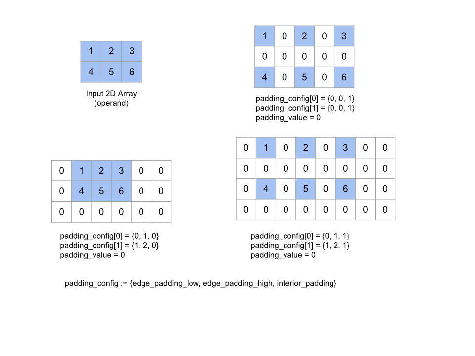
ขยายอาร์เรย์ operand ที่ระบุด้วยการเพิ่มระยะห่างจากขอบรอบอาร์เรย์ รวมถึงระหว่างองค์ประกอบของอาร์เรย์ด้วย padding_value ที่กำหนด padding_config จะระบุระยะห่างจากขอบและระยะห่างภายในของแต่ละมิติข้อมูล
PaddingConfig คือช่องที่ซ้ำของ PaddingConfigDimension ซึ่งมี 3 ช่องสำหรับแต่ละมิติข้อมูล ได้แก่ edge_padding_low, edge_padding_high และ interior_padding
edge_padding_low และ edge_padding_high จะระบุจำนวนระยะห่างจากขอบที่เพิ่มขึ้นในส่วนล่าง (ถัดจากดัชนี 0) และระดับไฮเอนด์ (ถัดจากดัชนีสูงสุด) ของแต่ละมิติข้อมูลตามลำดับ จำนวนระยะห่างจากขอบอาจเป็นค่าลบได้ ค่าสัมบูรณ์ของระยะห่างจากขอบเชิงลบจะระบุจำนวนองค์ประกอบที่จะนำออกจากมิติข้อมูลที่ระบุ
interior_padding ระบุระยะห่างจากขอบที่เพิ่มระหว่างองค์ประกอบ 2 รายการในแต่ละมิติข้อมูล โดยต้องไม่เป็นค่าลบ ระยะห่างจากขอบภายในเกิดขึ้นเชิงตรรกะก่อนระยะห่างจากขอบของขอบ ดังนั้นในกรณีที่มีระยะห่างจากขอบที่เป็นลบ องค์ประกอบจะถูกนำออกจากตัวถูกดำเนินการแบบบุนวมภายใน
การดำเนินการนี้จะไม่ดำเนินการหากคู่ระยะห่างจากขอบเป็นทั้งหมด (0, 0) และค่าระยะห่างจากขอบภายในเป็น 0 ทั้งหมด รูปด้านล่างแสดงตัวอย่างค่า edge_padding และ interior_padding ที่แตกต่างกันสำหรับอาร์เรย์ 2 มิติ
Recv
ดู XlaBuilder::Recv เพิ่มเติม
Recv(shape, channel_handle)
| อาร์กิวเมนต์ | ประเภท | อรรถศาสตร์ |
|---|---|---|
shape |
Shape |
รูปแบบของข้อมูลที่จะรับ |
channel_handle |
ChannelHandle |
ตัวระบุที่ไม่ซ้ำกันสำหรับคู่การส่ง/การรับแต่ละคู่ |
รับข้อมูลของรูปร่างที่ระบุจากคำสั่ง Send ในการคำนวณอื่นที่ใช้แฮนเดิลของช่องเดียวกัน แสดงผลเป็น
XlaOp สำหรับข้อมูลที่ได้รับ
API ไคลเอ็นต์ของการดำเนินการ Recv แสดงการสื่อสารพร้อมกัน
อย่างไรก็ตาม ระบบจะแยกวิธีการออกเป็น 2 คำสั่ง HLO (Recv และ RecvDone) ภายในเพื่อเปิดใช้การโอนข้อมูลแบบไม่พร้อมกัน ดูเพิ่มเติมที่ HloInstruction::CreateRecv และ HloInstruction::CreateRecvDone
Recv(const Shape& shape, int64 channel_id)
จัดสรรทรัพยากรที่จำเป็นต่อการรับข้อมูลจากคำสั่ง Send ที่มี channel_id เดียวกัน แสดงผลบริบทสำหรับทรัพยากรที่จัดสรรโดยใช้คำสั่ง RecvDone ต่อไปนี้เพื่อรอให้การโอนข้อมูลเสร็จสมบูรณ์ บริบทเป็น Tuple ของ {receiveทางธุรกิจ (รูปร่าง), ตัวระบุคำขอ (U32)} และสามารถใช้ได้โดยคำสั่ง RecvDone เท่านั้น
RecvDone(HloInstruction context)
ต้องรอให้การโอนข้อมูลเสร็จสมบูรณ์และส่งกลับข้อมูลที่ได้รับเมื่อมีบริบทที่คำสั่ง Recv สร้างขึ้น
ลด
ดู XlaBuilder::Reduce เพิ่มเติม
ใช้ฟังก์ชันการลดกับอาร์เรย์อย่างน้อย 1 รายการพร้อมกัน
Reduce(operands..., init_values..., computation, dimensions)
| อาร์กิวเมนต์ | ประเภท | อรรถศาสตร์ |
|---|---|---|
operands |
ลำดับของ N XlaOp |
N อาร์เรย์ประเภท T_0, ..., T_{N-1} |
init_values |
ลำดับของ N XlaOp |
สเกลาร์ N ของประเภท T_0, ..., T_{N-1} |
computation |
XlaComputation |
การคำนวณประเภท T_0, ..., T_{N-1}, T_0, ..., T_{N-1} -> Collate(T_0, ..., T_{N-1}) |
dimensions |
int64 อาร์เรย์ |
อาร์เรย์ที่ไม่เรียงลำดับของมิติข้อมูลที่จะลด |
โดยที่
- ต้องมี N มากกว่าหรือเท่ากับ 1
- การคำนวณจะต้องเชื่อมโยงกัน "คร่าวๆ" (ดูด้านล่าง)
- อาร์เรย์อินพุตทั้งหมดต้องมีขนาดเท่ากัน
- ค่าเริ่มต้นทั้งหมดต้องสร้างข้อมูลประจำตัวภายใต้
computation - หากเป็น
N = 1Collate(T)จะเท่ากับT - หากเป็น
N > 1Collate(T_0, ..., T_{N-1})จะเป็น Tuple ของNองค์ประกอบประเภทT
การดำเนินการนี้จะลดขนาดของอาร์เรย์อินพุตแต่ละรายการเป็นสเกลาร์
อันดับของอาร์เรย์ที่แสดงผลแต่ละรายการคือ rank(operand) - len(dimensions) เอาต์พุตของ op คือ Collate(Q_0, ..., Q_N) โดยที่ Q_i เป็นอาร์เรย์ของประเภท T_i โดยมีมิติข้อมูลที่อธิบายอยู่ด้านล่างนี้
แบ็กเอนด์ที่แตกต่างกันได้รับอนุญาตให้เชื่อมโยงการคำนวณการลดกลับเข้าไปใหม่ได้ ซึ่งอาจนำไปสู่ความแตกต่างด้านตัวเลข เนื่องจากฟังก์ชันการลดบางอย่าง เช่น การบวก ไม่เกี่ยวข้องกับการลอยตัว แต่หากช่วงของข้อมูลมีจำกัด การเพิ่มจุดลอยตัวก็ใกล้เคียงมากพอที่จะเชื่อมโยงสำหรับการใช้งานจริงส่วนใหญ่
ตัวอย่าง
เมื่อลดขนาดลงหนึ่งมิติข้อมูลในอาร์เรย์ 1D เดียวที่มีค่า [10, 11,
12, 13] ด้วยฟังก์ชันการลด f (คือ computation) อาจคํานวณเป็น
f(10, f(11, f(12, f(init_value, 13)))
แต่ก็ยังมีความเป็นไปได้อื่นๆ อีกมากมาย เช่น
f(init_value, f(f(10, f(init_value, 11)), f(f(init_value, 12), f(init_value, 13))))
ต่อไปนี้เป็นตัวอย่างรหัสเทียมแบบคร่าวๆ ว่าจะใช้การลดอย่างไร โดยใช้ผลรวมเป็นการคำนวณการลดที่มีค่าเริ่มต้นเป็น 0
result_shape <- remove all dims in dimensions from operand_shape

# Iterate over all elements in result_shape. The number of r's here is equal
# to the rank of the result
for r0 in range(result_shape[0]), r1 in range(result_shape[1]), ...:
  # Initialize this result element
  result[r0, r1...] <- 0

  # Iterate over all the reduction dimensions
  for d0 in range(dimensions[0]), d1 in range(dimensions[1]), ...:
    # Increment the result element with the value of the operand's element.
    # The index of the operand's element is constructed from all ri's and di's
    # in the right order (by construction ri's and di's together index over the
    # whole operand shape).
    result[r0, r1...] += operand[ri... di]
ต่อไปนี้เป็นตัวอย่างของการลดอาร์เรย์ 2 มิติ (เมทริกซ์) รูปร่างมีอันดับ 2 ขนาดที่ 2 และขนาดที่ 1 เท่ากับ 3
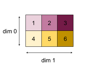
ผลลัพธ์ของการลดขนาด 0 หรือ 1 ด้วยฟังก์ชัน "เพิ่ม":
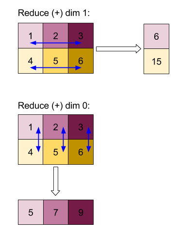
โปรดทราบว่าผลลัพธ์การลดทั้งสองเป็นอาร์เรย์ 1D แผนภาพนี้แสดงมุมมองหนึ่งเป็นคอลัมน์ และส่วนอีกแถวเป็นแถวเพื่อความสะดวก
สำหรับตัวอย่างที่ซับซ้อนยิ่งขึ้น นี่คืออาร์เรย์ 3 มิติ อันดับคือ 3 มิติข้อมูลขนาด 0 ของขนาด 4 มิติข้อมูลที่ 1 ของขนาด 2 และมิติข้อมูลที่ 2 ของขนาด 3 เพื่อให้เข้าใจได้ง่าย ระบบจะคัดลอกค่า 1 ถึง 6 ข้ามมิติข้อมูล 0
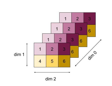
เช่นเดียวกับตัวอย่าง 2 มิติ เราสามารถลดมิติข้อมูลได้เพียงรายการเดียว เช่น หากเราลดมิติข้อมูล 0 เราจะได้อาร์เรย์อันดับ 2 ที่ค่าทั้งหมดในมิติข้อมูล 0 ถูกพับเป็นสเกลาร์ ดังนี้
|  4   8  12 |
| 16  20  24 |
หากเราลดมิติข้อมูล 2 เรายังได้รับอาร์เรย์อันดับ 2 ที่ค่าทั้งหมดในมิติข้อมูล 2 จะพับเป็นสเกลาร์ด้วย ดังนี้
| 6  15 |
| 6  15 |
| 6  15 |
| 6  15 |
โปรดทราบว่าระบบจะรักษาลำดับที่สัมพันธ์กันระหว่างมิติข้อมูลที่เหลือในอินพุต ไว้ในเอาต์พุต แต่มิติข้อมูลบางรายการอาจกำหนดตัวเลขใหม่ (เนื่องจากอันดับ มีการเปลี่ยนแปลง)
และยังสามารถลดขนาดลงได้หลายแบบ มิติข้อมูลการลดการเพิ่ม 0 และ 1 จะสร้างอาร์เรย์ 1 มิติ [20, 28, 36]
การลดอาร์เรย์ 3 มิติในมิติข้อมูลทั้งหมดจะสร้างสเกลาร์ 84
วาเรียดิก Reduce (Variadic Reduce)
เมื่อ N > 1 แอปพลิเคชันการลดฟังก์ชันจะซับซ้อนขึ้นเล็กน้อย เนื่องจากเป็นการนำไปใช้พร้อมกันกับอินพุตทั้งหมด ตัวถูกดำเนินการจะได้รับการจัดสรรสำหรับการคํานวณตามลำดับต่อไปนี้
- การเรียกใช้ค่าที่ลดลงสำหรับตัวถูกดำเนินการแรก
- ...
- การเรียกใช้ค่าที่ลดลงสำหรับตัวถูกดำเนินการ N
- ค่าที่ป้อนสำหรับตัวถูกดำเนินการแรก
- ...
- ค่าที่ป้อนสำหรับตัวถูกดำเนินการ N
ตัวอย่างเช่น ลองพิจารณาฟังก์ชันการลดต่อไปนี้ ซึ่งใช้ในการคำนวณค่าสูงสุดและ argmax ของอาร์เรย์ 1-D แบบขนานได้
f: (Float, Int, Float, Int) -> Float, Int
f(max, argmax, value, index):
  if value >= max:
    return (value, index)
  else:
    return (max, argmax)
สำหรับอาร์เรย์อินพุต 1-D ที่มี V = Float[N], K = Int[N] และค่าเริ่มต้น I_V = Float, I_K = Int ผลของการลด f_(N-1) ในมิติข้อมูลอินพุตเดียวจะเท่ากับแอปพลิเคชันแบบวนซ้ำต่อไปนี้
f_0 = f(I_V, I_K, V_0, K_0)
f_1 = f(f_0.first, f_0.second, V_1, K_1)
...
f_(N-1) = f(f_(N-2).first, f_(N-2).second, V_(N-1), K_(N-1))
การใช้การลดนี้กับอาร์เรย์ของค่า และอาร์เรย์ของดัชนีตามลำดับ (เช่น iota) จะทำซ้ำบนอาร์เรย์ และแสดง tuple ที่มีค่าสูงสุดและดัชนีที่ตรงกัน
ReducePrecision
ดู XlaBuilder::ReducePrecision เพิ่มเติม
สร้างแบบจำลองผลของการแปลงค่าจุดลอยตัวเป็นรูปแบบที่มีความแม่นยำต่ำกว่า (เช่น IEEE-FP16) และกลับไปเป็นรูปแบบเดิม สามารถระบุจำนวนบิตของเลขชี้กำลังและบิตแมนทิสซาในรูปแบบความแม่นยำต่ำกว่าได้ตามต้องการ แม้ว่าการใช้งานฮาร์ดแวร์บางรายการอาจไม่รองรับขนาดบิตทั้งหมด
ReducePrecision(operand, mantissa_bits, exponent_bits)
| อาร์กิวเมนต์ | ประเภท | อรรถศาสตร์ |
|---|---|---|
operand |
XlaOp |
อาร์เรย์ของประเภทจุดลอยตัว T |
exponent_bits |
int32 |
จำนวนบิตของเลขชี้กำลังในรูปแบบที่มีความแม่นยำต่ำ |
mantissa_bits |
int32 |
จำนวนบิตของ Mantissa ในรูปแบบที่มีความแม่นยำต่ำ |
ผลลัพธ์จะเป็นอาร์เรย์ประเภท T ระบบจะปัดเศษค่าอินพุตให้เป็นค่าที่ใกล้เคียงที่สุดที่แสดงด้วยจำนวนบิตของมันติสซาที่ระบุ (โดยใช้ความหมายของ "ที่เท่ากับคู่") และค่าที่เกินช่วงที่ระบุโดยจำนวนบิตของเลขชี้กำลังจะถูกบีบให้เป็นค่าอนันต์ที่เป็นบวกหรือลบ ค่า NaN จะยังคงอยู่ แม้ว่าระบบอาจแปลงเป็นค่า NaN ตามรูปแบบบัญญัติก็ตาม
รูปแบบที่มีความแม่นยำต่ำกว่าต้องมีเลขชี้กำลังอย่างน้อย 1 บิต (เพื่อแยกค่าศูนย์ออกจากค่าอนันต์ เนื่องจากทั้งสองค่ามีแมนติสซาเป็นศูนย์) และต้องมีจำนวนบิตของมันติสซาที่ไม่เป็นลบ จำนวนบิตของเลขชี้กำลังหรือไขมัน อาจเกินค่าที่เกี่ยวข้องสำหรับประเภท T ส่วนที่เกี่ยวข้องของ Conversion จะเป็นเพียงค่าที่ไม่มีตรงข้าม
ReduceScatter
ดู XlaBuilder::ReduceScatter เพิ่มเติม
ReduceScatter เป็นการดำเนินการร่วมที่ทำได้กับ AllReduce อย่างมีประสิทธิภาพ จากนั้นจะกระจายผลลัพธ์ด้วยการแยกผลลัพธ์เป็น shard_count บล็อกตาม
scatter_dimension และตัวจำลอง i ในกลุ่มตัวจำลองจะได้รับ
ชาร์ด ith
ReduceScatter(operand, computation, scatter_dim, shard_count,
replica_group_ids, channel_id)
| อาร์กิวเมนต์ | ประเภท | อรรถศาสตร์ |
|---|---|---|
operand |
XlaOp |
อาร์เรย์หรือ Tuple ของอาร์เรย์ที่ไม่ว่างเปล่าที่จะลดข้อมูลจำลอง |
computation |
XlaComputation |
การคํานวณการลด |
scatter_dimension |
int64 |
มิติข้อมูลที่จะกระจาย |
shard_count |
int64 |
จำนวนบล็อกที่จะแยก scatter_dimension |
replica_groups |
เวกเตอร์ของเวกเตอร์ของ int64 |
กลุ่มที่จะทำการลด |
channel_id |
ไม่บังคับ int64 |
รหัสแชแนลที่ไม่บังคับสำหรับการสื่อสารข้ามโมดูล |
- เมื่อ
operandเป็น Tuple ของอาร์เรย์ ระบบจะใช้การลดการกระจายกับแต่ละองค์ประกอบของ Tuple replica_groupsคือรายการของกลุ่มตัวจำลองที่ใช้ทำการลด (คุณจะเรียกข้อมูลรหัสการจำลองสำหรับตัวจำลองปัจจุบันได้โดยใช้ReplicaId) ลำดับของตัวจำลองในแต่ละกลุ่มจะกำหนดลำดับที่จะกระจายผลลัพธ์การลดทั้งหมดreplica_groupsต้องว่างเปล่า (ในกรณีนี้ตัวจำลองทั้งหมดจะเป็นของกลุ่มเดียว) หรือมีองค์ประกอบจำนวนเท่ากับจำนวนตัวจำลอง เมื่อมีกลุ่มตัวจำลองมากกว่า 1 กลุ่ม ทุกกลุ่มต้องมีขนาดเท่ากัน เช่นreplica_groups = {0, 2}, {1, 3}จะลดจำนวนตัวจำลอง0กับ2รวมถึง1และ3แล้วกระจายผลลัพธ์shard_countคือขนาดของกลุ่มตัวจำลองแต่ละกลุ่ม เราต้องการข้อมูลนี้ในกรณีที่replica_groupsว่างเปล่า หากreplica_groupsมีข้อมูลอยู่shard_countต้องเท่ากับขนาดของกลุ่มตัวจำลองแต่ละกลุ่มchannel_idใช้สำหรับการสื่อสารข้ามโมดูล: มีเพียงreduce-scatterการดำเนินการที่มีchannel_idเดียวกันเท่านั้นที่สามารถสื่อสารกันได้
รูปร่างเอาต์พุตคือรูปร่างอินพุตที่มี scatter_dimension ทำให้เล็กลง shard_count เท่า เช่น หากมีตัวจำลอง 2 รายการและตัวถูกดำเนินการมีค่า [1.0, 2.25] และ [3.0, 5.25] ในตัวจำลอง 2 ตัวตามลำดับ ค่าเอาต์พุตจากตัวจำลองนี้ที่ scatter_dim คือ 0 จะเป็น [4.0] สำหรับตัวจำลองแรก และ [7.5] สำหรับตัวจำลองที่ 2
ReduceWindow
ดู XlaBuilder::ReduceWindow เพิ่มเติม
ใช้ฟังก์ชันการลดรูปกับองค์ประกอบทั้งหมดในแต่ละหน้าต่างของอาร์เรย์ N หลายมิติข้อมูลตามลำดับ โดยสร้างอาร์เรย์หลายมิติ N เดี่ยวหรือ 1 ชุดเป็นเอาต์พุต อาร์เรย์เอาต์พุตแต่ละรายการมีจำนวนองค์ประกอบเท่ากับจำนวนตำแหน่งที่ถูกต้องของหน้าต่าง เลเยอร์พูลสามารถแสดงเป็น ReduceWindow เช่นเดียวกับ Reduce computationที่ใช้จะส่งผ่าน init_values ทางด้านซ้ายเสมอ
ReduceWindow(operands..., init_values..., computation, window_dimensions,
window_strides, padding)
| อาร์กิวเมนต์ | ประเภท | อรรถศาสตร์ |
|---|---|---|
operands |
N XlaOps |
ลำดับของอาร์เรย์หลายมิติ N ของประเภท T_0,..., T_{N-1} โดยแต่ละอาร์เรย์จะแสดงพื้นที่ฐานที่มีการวางหน้าต่าง |
init_values |
N XlaOps |
ค่าเริ่มต้นของ N สำหรับการลด 1 ค่าต่อตัวถูกดำเนินการ N แต่ละค่า ดูรายละเอียดได้ที่ลด |
computation |
XlaComputation |
ฟังก์ชันการลดประเภท T_0, ..., T_{N-1}, T_0, ..., T_{N-1} -> Collate(T_0, ..., T_{N-1}) เพื่อใช้กับองค์ประกอบในแต่ละหน้าต่างของตัวถูกดำเนินการอินพุตทั้งหมด |
window_dimensions |
ArraySlice<int64> |
อาร์เรย์ของจำนวนเต็มสำหรับค่ามิติข้อมูลหน้าต่าง |
window_strides |
ArraySlice<int64> |
อาร์เรย์ของจำนวนเต็มสำหรับค่าการก้าวหน้าต่าง |
base_dilations |
ArraySlice<int64> |
อาร์เรย์ของจำนวนเต็มสำหรับค่าการขยายฐาน |
window_dilations |
ArraySlice<int64> |
อาร์เรย์ของจำนวนเต็มสำหรับค่าการขยายหน้าต่าง |
padding |
Padding |
ประเภทระยะห่างจากขอบสำหรับหน้าต่าง (ระยะห่างจากขอบ::kSame ซึ่งเป็นแพดที่ทำให้มีรูปร่างเอาต์พุตเดียวกันกับอินพุตในกรณีที่การก้าวเป็น 1 หรือ Padding::kValid ซึ่งไม่มีระยะห่างจากขอบและ "หยุด" หน้าต่างเมื่อไม่พอดีกับหน้าอีกต่อไป) |
โดยที่
- ต้องมี N มากกว่าหรือเท่ากับ 1
- อาร์เรย์อินพุตทั้งหมดต้องมีขนาดเท่ากัน
- หากเป็น
N = 1Collate(T)จะเท่ากับT - หากเป็น
N > 1Collate(T_0, ..., T_{N-1})จะเป็น Tuple ของNองค์ประกอบประเภท(T0,...T{N-1})
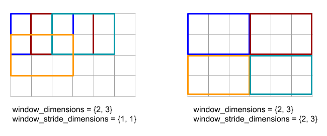
โค้ดและรูปด้านล่างแสดงตัวอย่างการใช้ ReduceWindow อินพุตคือเมทริกซ์ขนาด [4x6] และทั้ง window_dimensions และ window_stride_dimensions คือ [2x3]
// Create a computation for the reduction (maximum).
XlaComputation max;
{
  XlaBuilder builder(client_, "max");
  auto y = builder.Parameter(0, ShapeUtil::MakeShape(F32, {}), "y");
  auto x = builder.Parameter(1, ShapeUtil::MakeShape(F32, {}), "x");
  builder.Max(y, x);
  max = builder.Build().value();
}

// Create a ReduceWindow computation with the max reduction computation.
XlaBuilder builder(client_, "reduce_window_2x3");
auto shape = ShapeUtil::MakeShape(F32, {4, 6});
auto input = builder.Parameter(0, shape, "input");
builder.ReduceWindow(
    input,
    /*init_val=*/builder.ConstantLiteral(LiteralUtil::MinValue(F32)),
    *max,
    /*window_dimensions=*/{2, 3},
    /*window_stride_dimensions=*/{2, 3},
    Padding::kValid);
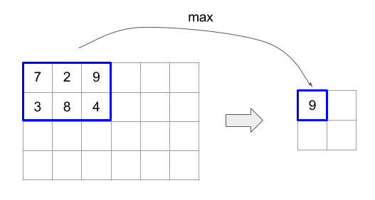
จังหวะของ 1 ในมิติข้อมูลเป็นการระบุว่าตำแหน่งของหน้าต่างในมิติข้อมูลอยู่ห่างจากหน้าต่างที่อยู่ติดกัน 1 องค์ประกอบ ในการระบุว่าไม่มีหน้าต่างใดซ้อนทับกัน หน้าต่าง_stride_dimensions ควรเท่ากับwindow_dimensions รูปด้านล่างแสดงให้เห็นการใช้ ค่าพัฒนาการที่แตกต่างกัน 2 ค่า การเพิ่มระยะห่างจากขอบจะใช้กับมิติข้อมูลแต่ละรายการของอินพุต และการคำนวณจะเหมือนกับอินพุตที่มาพร้อมกับมิติข้อมูลที่มีหลังระยะห่างจากขอบ
สำหรับตัวอย่างระยะห่างจากขอบที่ไม่สำคัญ ลองพิจารณาการประมวลผลการลดหน้าต่างขั้นต่ำ
(ค่าเริ่มต้นคือ MAX_FLOAT) ด้วยมิติข้อมูล 3 และก้าว 2 เหนืออาร์เรย์อินพุต [10000, 1000, 100, 10, 1] การเพิ่มระยะห่างจากขอบของ kValid จะคำนวณต่ำสุดใน 2 กรอบเวลาที่ถูกต้อง ได้แก่ [10000, 1000, 100] และ [100, 10, 1] ซึ่งทําให้เอาต์พุตเป็น [100, 1] ก่อนอื่น ระยะห่างจากขอบของ kSame จะแพ็คอาร์เรย์เพื่อให้รูปร่างหลังหน้าต่างการลดเป็นเดียวกับอินพุตสำหรับจังหวะการก้าวด้วยการเพิ่มองค์ประกอบเริ่มต้นทั้ง 2 ด้าน จะได้ [MAX_VALUE, 10000, 1000, 100, 10, 1,
MAX_VALUE] การเรียกใช้กรอบเวลาการลดบนอาร์เรย์เบาะจะทำงานบน 3 หน้าต่าง [MAX_VALUE, 10000, 1000], [1000, 100, 10], [10, 1, MAX_VALUE] และผลตอบแทน [1000, 10, 1]
ลำดับการประเมินของฟังก์ชันการลดเป็นกฎเกณฑ์และอาจไม่ได้กำหนด ดังนั้น ฟังก์ชันการลดจึงไม่ควรคำนึงถึง
การเชื่อมโยงใหม่มากเกินไป ดูรายละเอียดเพิ่มเติมได้ที่การสนทนาเกี่ยวกับการเชื่อมโยงในบริบทของ Reduce
ReplicaId
ดู XlaBuilder::ReplicaId เพิ่มเติม
แสดงผลรหัสที่ไม่ซ้ำกัน (สเกลาร์ U32) ของตัวจำลอง
ReplicaId()
รหัสที่ไม่ซ้ำกันของตัวจำลองแต่ละรายการคือจำนวนเต็มที่ไม่มีเครื่องหมายในช่วง [0, N) โดย N คือจำนวนตัวจำลอง เนื่องจากตัวจำลองทั้งหมดเรียกใช้โปรแกรมเดียวกัน การเรียก ReplicaId() ในโปรแกรมจะแสดงผลค่าที่แตกต่างกันบนตัวจำลองแต่ละตัว
ปรับรูปร่าง
โปรดดูเพิ่มเติมที่ XlaBuilder::Reshape และการดําเนินการ Collapse
เปลี่ยนรูปร่างของอาร์เรย์เป็นการกำหนดค่าใหม่
Reshape(operand, new_sizes)
Reshape(operand, dimensions, new_sizes)
| อาร์กิวเมนต์ | ประเภท | อรรถศาสตร์ |
|---|---|---|
operand |
XlaOp |
อาร์เรย์ประเภท T |
dimensions |
int64 เวกเตอร์ |
ลำดับการยุบมิติข้อมูล |
new_sizes |
int64 เวกเตอร์ |
เวกเตอร์ของขนาดของมิติข้อมูลใหม่ |
โดยหลักการแล้ว ปรับรูปร่างให้แบนอาร์เรย์เป็นเวกเตอร์ 1 มิติของค่าข้อมูลก่อน แล้วจึงปรับแต่งเวกเตอร์นี้เป็นรูปร่างใหม่ อาร์กิวเมนต์อินพุตคืออาร์เรย์ที่กำหนดเองของประเภท T ซึ่งเป็นเวกเตอร์ค่าคงที่เวลาคอมไพล์ของดัชนีมิติข้อมูล และเวกเตอร์คงที่เวลาคอมไพล์ของขนาดมิติข้อมูลสำหรับผลลัพธ์
ค่าในเวกเตอร์ dimension หากมีค่า จะต้องเป็นการเรียงสับเปลี่ยนมิติข้อมูลของ T ทั้งหมด ค่าเริ่มต้นหากไม่ได้กำหนดคือ {0, ..., rank - 1} ลำดับของมิติข้อมูลใน dimensions คือจากมิติข้อมูลที่เปลี่ยนแปลงช้าที่สุด (สำคัญที่สุด) ไปจนถึงมิติข้อมูลที่เปลี่ยนแปลงเร็วที่สุด (มีน้อยสุด) ใน Nest Loop ซึ่งยุบอาร์เรย์อินพุตเป็นมิติข้อมูลเดียว เวกเตอร์ new_sizes จะเป็นตัวกำหนดขนาดของอาร์เรย์เอาต์พุต ค่าที่ดัชนี 0 ใน new_sizes คือขนาดมิติข้อมูล 0 ค่าที่ดัชนี 1 คือขนาดของมิติข้อมูล 1 เป็นต้น ผลลัพธ์ของมิติข้อมูล new_size ต้องเท่ากับผลคูณของขนาดตัวถูกดำเนินการ เมื่อปรับแต่งอาร์เรย์ที่ยุบเป็นอาร์เรย์หลายมิติที่กำหนดโดย new_sizes มิติข้อมูลใน new_sizes จะเรียงลำดับจากหลายมิติช้าที่สุด (ใหญ่ที่สุด) ไปจนถึงแปรผันเร็วที่สุด (น้อยที่สุด)
ตัวอย่างเช่น กำหนดให้ v เป็นอาร์เรย์ขององค์ประกอบ 24 รายการ
let v = f32[4x2x3] { { {10, 11, 12}, {15, 16, 17} },
                    { {20, 21, 22}, {25, 26, 27} },
                    { {30, 31, 32}, {35, 36, 37} },
                    { {40, 41, 42}, {45, 46, 47} } };

In-order collapse:
let v012_24 = Reshape(v, {0,1,2}, {24});
then v012_24 == f32[24] {10, 11, 12, 15, 16, 17, 20, 21, 22, 25, 26, 27,
                         30, 31, 32, 35, 36, 37, 40, 41, 42, 45, 46, 47};

let v012_83 = Reshape(v, {0,1,2}, {8,3});
then v012_83 == f32[8x3] { {10, 11, 12}, {15, 16, 17},
                          {20, 21, 22}, {25, 26, 27},
                          {30, 31, 32}, {35, 36, 37},
                          {40, 41, 42}, {45, 46, 47} };

Out-of-order collapse:
let v021_24 = Reshape(v, {1,2,0}, {24});
then v012_24 == f32[24]  {10, 20, 30, 40, 11, 21, 31, 41, 12, 22, 32, 42,
                          15, 25, 35, 45, 16, 26, 36, 46, 17, 27, 37, 47};

let v021_83 = Reshape(v, {1,2,0}, {8,3});
then v021_83 == f32[8x3] { {10, 20, 30}, {40, 11, 21},
                          {31, 41, 12}, {22, 32, 42},
                          {15, 25, 35}, {45, 16, 26},
                          {36, 46, 17}, {27, 37, 47} };


let v021_262 = Reshape(v, {1,2,0}, {2,6,2});
then v021_262 == f32[2x6x2] { { {10, 20}, {30, 40},
                              {11, 21}, {31, 41},
                              {12, 22}, {32, 42} },
                             { {15, 25}, {35, 45},
                              {16, 26}, {36, 46},
                              {17, 27}, {37, 47} } };
ในบางกรณีพิเศษ การปรับรูปร่างสามารถเปลี่ยนอาร์เรย์องค์ประกอบเดียวเป็นสเกลาร์ได้ และในทางกลับกันด้วย ตัวอย่างเช่น
Reshape(f32[1x1] { {5} }, {0,1}, {}) == 5;
Reshape(5, {}, {1,1}) == f32[1x1] { {5} };
รายได้ (ย้อนกลับ)
ดู XlaBuilder::Rev เพิ่มเติม
Rev(operand, dimensions)
| อาร์กิวเมนต์ | ประเภท | อรรถศาสตร์ |
|---|---|---|
operand |
XlaOp |
อาร์เรย์ประเภท T |
dimensions |
ArraySlice<int64> |
มิติข้อมูลที่จะย้อนกลับ |
ย้อนลำดับองค์ประกอบในอาร์เรย์ operand ตาม dimensions ที่ระบุ เพื่อสร้างอาร์เรย์เอาต์พุตที่มีรูปทรงเดียวกัน องค์ประกอบแต่ละรายการของอาร์เรย์ตัวถูกดำเนินการในดัชนีหลายมิติจะได้รับการจัดเก็บไว้ในอาร์เรย์เอาต์พุตในดัชนีที่มีการเปลี่ยนรูปแบบ ดัชนีหลายมิติจะเปลี่ยนรูปแบบโดยการกลับดัชนีในแต่ละมิติข้อมูลเพื่อกลับด้าน (กล่าวคือ หากมิติข้อมูลขนาด N เป็นหนึ่งในมิติข้อมูลกลับด้าน ดัชนี i ของดัชนี i จะเปลี่ยนเป็น N - 1 - i)
การใช้งานอย่างหนึ่งสำหรับการดำเนินการ Rev คือการกลับอาร์เรย์น้ำหนักคอนโวลูชันตามมิติข้อมูลของหน้าต่าง 2 ด้านระหว่างการคำนวณการไล่ระดับสีในโครงข่ายระบบประสาทเทียม
RngNormal
ดู XlaBuilder::RngNormal เพิ่มเติม
สร้างเอาต์พุตของรูปร่างที่กำหนดด้วยตัวเลขสุ่มที่สร้างขึ้นตาม \(N(\mu, \sigma)\) การกระจายปกติ พารามิเตอร์ \(\mu\) และ \(\sigma\)และรูปร่างเอาต์พุตต้องมีประเภทองค์ประกอบที่เป็นจุดลอยตัว พารามิเตอร์อื่นๆ ต้องมีค่าแบบสเกลาร์ด้วย
RngNormal(mu, sigma, shape)
| อาร์กิวเมนต์ | ประเภท | อรรถศาสตร์ |
|---|---|---|
mu |
XlaOp |
สเกลาร์ของประเภท T ที่ระบุค่าเฉลี่ยของตัวเลขที่สร้างขึ้น |
sigma |
XlaOp |
สเกลาร์ของประเภท T ที่ระบุส่วนเบี่ยงเบนมาตรฐานของประเภท T |
shape |
Shape |
รูปร่างเอาต์พุตประเภท T |
RngUniform
ดู XlaBuilder::RngUniform เพิ่มเติม
สร้างเอาต์พุตของรูปร่างที่กำหนดด้วยตัวเลขสุ่มที่สร้างขึ้นหลังจากการกระจายที่สม่ำเสมอในช่วง \([a,b)\)พารามิเตอร์และประเภทองค์ประกอบเอาต์พุตต้องเป็นประเภทบูลีน ประเภทปริพันธ์หรือประเภทจุดลอยตัว และประเภทต้องสอดคล้องกัน ปัจจุบันแบ็กเอนด์ของ CPU และ GPU รองรับเฉพาะ F64, F32, F16, BF16, S64, U64, S32 และ U32 เท่านั้น นอกจากนี้ พารามิเตอร์ต้องมีค่าแบบสเกลาร์ ถ้า \(b <= a\) ผลลัพธ์ที่ได้คือ มีการกำหนดการใช้งาน
RngUniform(a, b, shape)
| อาร์กิวเมนต์ | ประเภท | อรรถศาสตร์ |
|---|---|---|
a |
XlaOp |
สเกลาร์ของประเภท T ที่ระบุขีดจำกัดต่ำสุดของช่วงเวลา |
b |
XlaOp |
สเกลาร์ของประเภท T ที่ระบุขีดจำกัดบนของช่วง |
shape |
Shape |
รูปร่างเอาต์พุตประเภท T |
RngBitGenerator
สร้างเอาต์พุตด้วยรูปร่างที่กำหนดซึ่งเต็มไปด้วยบิตแบบสุ่มที่สม่ำเสมอโดยใช้อัลกอริทึมที่ระบุ (หรือค่าเริ่มต้นของแบ็กเอนด์) และแสดงผลสถานะที่อัปเดต (โดยมีรูปร่างเดียวกันกับสถานะเริ่มต้น) รวมถึงข้อมูลแบบสุ่มที่สร้างขึ้น
สถานะเริ่มต้นคือสถานะเริ่มต้นของการสร้างหมายเลขสุ่มในปัจจุบัน โดยรูปร่างที่กำหนดและค่าที่ถูกต้องจะขึ้นอยู่กับอัลกอริทึมที่ใช้
เอาต์พุตเหล่านี้รับประกันได้ว่าเป็นฟังก์ชันเชิงกำหนดของสถานะเริ่มต้น แต่ก็ไม่รับประกันว่าจะมีการกำหนดระหว่างแบ็กเอนด์และเวอร์ชันคอมไพเลอร์ที่แตกต่างกัน
RngBitGenerator(algorithm, key, shape)
| อาร์กิวเมนต์ | ประเภท | อรรถศาสตร์ |
|---|---|---|
algorithm |
RandomAlgorithm |
อัลกอริทึม PRNG ที่จะใช้ |
initial_state |
XlaOp |
สถานะเริ่มต้นสำหรับอัลกอริทึม PRNG |
shape |
Shape |
รูปร่างเอาต์พุตสำหรับข้อมูลที่สร้างขึ้น |
ค่าที่ใช้ได้สำหรับ algorithm:
rng_default: อัลกอริทึมเฉพาะของแบ็กเอนด์ที่มีข้อกำหนดรูปร่างที่เจาะจงของแบ็กเอนด์rng_three_fry: อัลกอริทึม PRNG แบบอิงตามตัวนับ ThreeFry รูปร่างinitial_stateคือu64[2]ที่มีค่าที่กำหนดเอง Salmon et al. SC 2011 เลขสุ่มคู่ขนาน: ง่ายเหมือนนับ 1, 2, 3rng_philox: อัลกอริทึม Philox ในการสร้างตัวเลขสุ่มคู่ขนาน รูปร่างinitial_stateคือu64[3]ที่มีค่าที่กำหนดเอง Salmon et al. SC 2011 เลขสุ่มคู่ขนาน: ง่ายเหมือนนับ 1, 2, 3
แผนภูมิกระจาย
การดำเนินการกระจาย XLA จะสร้างผลลัพธ์ตามลำดับซึ่งเป็นค่าของอาร์เรย์อินพุต operands โดยหลายชิ้นส่วน (ที่ดัชนีที่ระบุโดย scatter_indices) อัปเดตลำดับของค่าใน updates โดยใช้ update_computation
ดู XlaBuilder::Scatter เพิ่มเติม
scatter(operands..., scatter_indices, updates..., update_computation,
index_vector_dim, update_window_dims, inserted_window_dims,
scatter_dims_to_operand_dims)
| อาร์กิวเมนต์ | ประเภท | อรรถศาสตร์ |
|---|---|---|
operands |
ลำดับของ N XlaOp |
อาร์เรย์ N อาร์เรย์ของประเภท T_0, ..., T_N ที่จะกระจายไปยัง |
scatter_indices |
XlaOp |
อาร์เรย์ที่มีดัชนีเริ่มต้นของชิ้นส่วนที่ต้องกระจายอยู่ |
updates |
ลำดับของ N XlaOp |
N อาร์เรย์ประเภท T_0, ..., T_N updates[i] มีค่าที่ต้องใช้สำหรับการกระจาย operands[i] |
update_computation |
XlaComputation |
การคำนวณที่จะใช้ในการรวมค่าที่มีอยู่ในอาร์เรย์อินพุตและการอัปเดตระหว่างการกระจาย การคำนวณนี้ควรเป็นประเภท T_0, ..., T_N, T_0, ..., T_N -> Collate(T_0, ..., T_N) |
index_vector_dim |
int64 |
มิติข้อมูลใน scatter_indices ที่มีดัชนีเริ่มต้น |
update_window_dims |
ArraySlice<int64> |
ชุดของมิติข้อมูลในรูปร่าง updates ที่เป็นมิติข้อมูลหน้าต่าง |
inserted_window_dims |
ArraySlice<int64> |
ชุดขนาดหน้าต่างที่ต้องแทรกในรูปร่าง updates |
scatter_dims_to_operand_dims |
ArraySlice<int64> |
การจับคู่มิติข้อมูลจากดัชนีกระจายไปยังพื้นที่ดัชนีตัวถูกดำเนินการ ระบบตีความอาร์เรย์นี้เป็นการแมป i กับ scatter_dims_to_operand_dims[i] ซึ่งจะต้องเป็นแบบ 1 ต่อ 1 และทั้งหมด |
indices_are_sorted |
bool |
ดูว่าผู้โทรน่าจะจัดเรียงดัชนีหรือไม่ |
โดยที่
- ต้องมี N มากกว่าหรือเท่ากับ 1
operands[0], ...,operands[N-1] ทั้งหมดต้องมีมิติข้อมูลเดียวกันupdates[0], ...,updates[N-1] ทั้งหมดต้องมีมิติข้อมูลเดียวกัน- หากเป็น
N = 1Collate(T)จะเท่ากับT - หาก
N > 1Collate(T_0, ..., T_N)เป็น Tuple ของNองค์ประกอบประเภทT
หาก index_vector_dim เท่ากับ scatter_indices.rank เราจะถือว่า scatter_indices มีมิติข้อมูล 1 ต่อท้าย
เราให้คำจำกัดความ update_scatter_dims ของประเภท ArraySlice<int64> เป็นชุดมิติข้อมูลในรูปร่าง updates ที่ไม่ได้อยู่ใน update_window_dims โดยเรียงลำดับจากน้อยไปหามาก
อาร์กิวเมนต์ของการกระจายควรเป็นไปตามข้อจำกัดต่อไปนี้
อาร์เรย์
updatesแต่ละอาร์เรย์ต้องมีอันดับupdate_window_dims.size + scatter_indices.rank - 1ขอบเขตของมิติข้อมูล
iในอาร์เรย์updatesแต่ละรายการต้องสอดคล้องกับข้อมูลต่อไปนี้- หาก
iอยู่ในupdate_window_dims(นั่นคือ เท่ากับupdate_window_dims[k] สำหรับkบางส่วน) ขอบเขตของมิติข้อมูลiในupdatesต้องไม่เกินขอบเขตที่เกี่ยวข้องของoperandหลังจากคำนวณinserted_window_dims(นั่นคือadjusted_window_bounds[k] โดยที่adjusted_window_boundsมีขอบเขตของoperandโดยมีขอบเขตของดัชนีinserted_window_dimsถูกนำออก) - หาก
iแสดงในupdate_scatter_dims(นั่นคือ เท่ากับupdate_scatter_dims[k] สําหรับkบางส่วน) ขอบเขตของมิติข้อมูลiในupdatesจะต้องเท่ากับขอบเขตที่สัมพันธ์กันของscatter_indicesซึ่งจะข้ามindex_vector_dim(กล่าวคือscatter_indices.shape.dims[k] แต่หากเป็นk<index_vector_dimและscatter_indices.shape.dims[k+1] ในกรณีอื่นๆ)
- หาก
update_window_dimsต้องเรียงจากน้อยไปมาก ไม่มีหมายเลขมิติข้อมูลซ้ำ และอยู่ในช่วง[0, updates.rank)inserted_window_dimsต้องเรียงจากน้อยไปมาก ไม่มีหมายเลขมิติข้อมูลซ้ำ และอยู่ในช่วง[0, operand.rank)operand.rankต้องเท่ากับผลรวมของupdate_window_dims.sizeและinserted_window_dims.sizescatter_dims_to_operand_dims.sizeต้องเท่ากับscatter_indices.shape.dims[index_vector_dim] และค่าต้องอยู่ในช่วง[0, operand.rank)
สำหรับดัชนี U ที่ระบุในอาร์เรย์ updates แต่ละอาร์เรย์ ระบบจะคำนวณดัชนีที่เกี่ยวข้อง I ในอาร์เรย์ operands ที่เกี่ยวข้องซึ่งใช้การอัปเดตนี้ดังนี้
- ให้
G= {U[k] สำหรับkในupdate_scatter_dims} ใช้Gเพื่อค้นหาเวกเตอร์ดัชนีSในอาร์เรย์scatter_indicesที่S[i] =scatter_indices[รวม(G,i)] โดยที่ "รวม(A, b) จะแทรก b ในตำแหน่งindex_vector_dimลงใน A - สร้างดัชนี
Sinลงในoperandโดยใช้SโดยการกระจายSโดยใช้แมปscatter_dims_to_operand_dimsเป็นทางการมากขึ้นSin[scatter_dims_to_operand_dims[k]] =S[k] หากk<scatter_dims_to_operand_dims.sizeSin[_] =0หากไม่ใช่
- สร้างดัชนี
Winลงในอาร์เรย์operandsแต่ละอาร์เรย์โดยกระจายดัชนีที่update_window_dimsในUตามinserted_window_dimsเป็นทางการมากขึ้นWin[window_dims_to_operand_dims(k)] =U[k] หากkอยู่ในupdate_window_dimsโดยที่window_dims_to_operand_dimsเป็นฟังก์ชันโมโนโทนิกที่มีโดเมน [0,update_window_dims.size) และ ช่วง [0,operand.rank) \inserted_window_dims(เช่น หากupdate_window_dims.sizeคือ4,operand.rankคือ6และinserted_window_dimsคือ {0,2} ดังนั้นwindow_dims_to_operand_dimsจะเป็น {0→1,1→3,2→4,3→5})Win[_] =0หากไม่ใช่
IคือWin+Sinโดยที่ + คือส่วนเพิ่มตามองค์ประกอบ
โดยสรุปแล้ว การกระจายดังกล่าวจะกำหนดได้ดังนี้
- เริ่มต้น
outputด้วยoperandsนั่นคือ สำหรับดัชนีทั้งหมดJสำหรับดัชนีทั้งหมดOในอาร์เรย์operands[J]:
output[J][O] =operands[J][O] - สำหรับดัชนี
Uทุกรายการในอาร์เรย์updates[J] และดัชนีที่สัมพันธ์กันOในอาร์เรย์operand[J] หากOเป็นดัชนีที่ถูกต้องสำหรับoutput:
(output[0][O], ...,output[N-1][O]) =update_computation(output[0][O], ..., ,output[N-1][O],updates[0][U], ...,updates[N-1][U])
ไม่สามารถกำหนดลำดับการอัปเดตได้ ดังนั้น เมื่อดัชนีหลายรายการใน updates อ้างอิงดัชนีเดียวกันใน operands จะไม่มีการกำหนดค่าที่ตรงกันใน output
โปรดทราบว่าพารามิเตอร์แรกที่ส่งเข้าไปใน update_computation จะเป็นค่าปัจจุบันจากอาร์เรย์ output เสมอ และพารามิเตอร์ที่ 2 จะเป็นค่าจากอาร์เรย์ updates เสมอ ซึ่งสำคัญโดยเฉพาะอย่างยิ่งในกรณีที่ update_computation ใช้สลับกันได้
หากตั้งค่า indices_are_sorted เป็น "จริง" XLA จะถือว่าผู้ใช้จัดเรียง start_indices (ตามลำดับจากน้อยไปมาก start_index_map) หากไม่เป็นเช่นนั้น ความหมายคือ "การนำไปใช้งาน"
อย่างไม่เป็นทางการ จะมองว่าการกระจายข้อมูลเป็นผกผันของ op ของการรวม กล่าวคือ การประมวลผลของการกระจายจะอัปเดตองค์ประกอบในอินพุตที่แยกโดย op ของการรวบรวมที่เกี่ยวข้อง
ดูคำอธิบายและตัวอย่างแบบไม่เป็นทางการโดยละเอียดที่
ส่วน "คำอธิบายอย่างไม่เป็นทางการ" ใต้ Gather
เลือก
ดู XlaBuilder::Select เพิ่มเติม
สร้างอาร์เรย์เอาต์พุตจากองค์ประกอบของอาร์เรย์อินพุต 2 รายการ โดยอิงตามค่าของอาร์เรย์เพรดิเคต
Select(pred, on_true, on_false)
| อาร์กิวเมนต์ | ประเภท | อรรถศาสตร์ |
|---|---|---|
pred |
XlaOp |
อาร์เรย์ประเภท PRED |
on_true |
XlaOp |
อาร์เรย์ประเภท T |
on_false |
XlaOp |
อาร์เรย์ประเภท T |
อาร์เรย์ on_true และ on_false ต้องมีรูปทรงเดียวกัน นี่เป็นรูปร่างของอาร์เรย์เอาต์พุตด้วย อาร์เรย์ pred ต้องมีมิติข้อมูลเดียวกันกับ on_true และ on_false โดยมีประเภทองค์ประกอบ PRED
สำหรับองค์ประกอบ P แต่ละรายการของ pred องค์ประกอบที่สอดคล้องของอาร์เรย์เอาต์พุตจะนำมาจาก on_true หากค่าของ P คือ true และจาก on_false หากค่าของ P คือ false ในรูปแบบที่จำกัดของการออกอากาศ pred อาจเป็นสเกลาร์ประเภท PRED ในกรณีนี้ อาร์เรย์เอาต์พุตจะมาจาก on_true ทั้งหมดหาก pred คือ true และจาก on_false หาก pred คือ false
ตัวอย่างที่มี pred ที่ไม่ใช่สเกลาร์
let pred: PRED[4] = {true, false, false, true};
let v1: s32[4] = {1, 2, 3, 4};
let v2: s32[4] = {100, 200, 300, 400};
==>
Select(pred, v1, v2) = s32[4]{1, 200, 300, 4};
ตัวอย่างที่มีสเกลาร์ pred
let pred: PRED = true;
let v1: s32[4] = {1, 2, 3, 4};
let v2: s32[4] = {100, 200, 300, 400};
==>
Select(pred, v1, v2) = s32[4]{1, 2, 3, 4};
ระบบรองรับตัวเลือก Tuple ด้วย Tuple ถือเป็นประเภทสเกลาร์สำหรับจุดประสงค์นี้ หาก on_true และ on_false เป็น Tuples (ซึ่งต้องมีรูปร่างเหมือนกัน) pred จะต้องเป็นสเกลาร์ประเภท PRED
SelectAndScatter
ดู XlaBuilder::SelectAndScatter เพิ่มเติม
การดำเนินการนี้ถือเป็นการดำเนินการแบบผสมที่จะคำนวณ ReduceWindow ในอาร์เรย์ operand เพื่อเลือกองค์ประกอบจากแต่ละหน้าต่างก่อน จากนั้นกระจายอาร์เรย์ source ไปยังดัชนีขององค์ประกอบที่เลือกเพื่อสร้างอาร์เรย์เอาต์พุตที่มีรูปร่างเดียวกันกับอาร์เรย์โอเปอแรนด์ ฟังก์ชัน select สำหรับไบนารีนั้นใช้เพื่อเลือกองค์ประกอบจากแต่ละหน้าต่างโดยนำไปใช้กับแต่ละหน้าต่าง และมีการเรียกใช้ด้วยคุณสมบัติว่าเวกเตอร์ดัชนีของพารามิเตอร์แรกน้อยกว่าเวกเตอร์ดัชนีแบบพจนานุกรม ฟังก์ชัน select จะแสดงผล true หากเลือกพารามิเตอร์แรกและแสดงผล false หากเลือกพารามิเตอร์ที่ 2 และฟังก์ชันต้องคงการรับส่ง (เช่น หาก select(a, b) และ select(b, c) เป็น true แล้ว select(a, c) จะเป็น true ด้วย) เพื่อให้องค์ประกอบที่เลือกไม่ขึ้นอยู่กับลำดับขององค์ประกอบที่ข้ามผ่านสำหรับหน้าต่างที่ระบุ
ระบบจะใช้ฟังก์ชัน scatter ที่ดัชนีที่เลือกแต่ละรายการในอาร์เรย์เอาต์พุต ต้องใช้พารามิเตอร์สเกลาร์ 2 ตัว ได้แก่
- ค่าปัจจุบันที่ดัชนีที่เลือกในอาร์เรย์เอาต์พุต
- ค่ากระจายจาก
sourceที่ใช้กับดัชนีที่เลือก
โดยจะรวมพารามิเตอร์ 2 ตัวเข้าด้วยกันและแสดงผลค่าสเกลาร์ที่ใช้เพื่ออัปเดตค่าในดัชนีที่เลือกในอาร์เรย์เอาต์พุต ในช่วงแรก ดัชนีทั้งหมดของอาร์เรย์เอาต์พุตจะตั้งค่าเป็น init_value
อาร์เรย์เอาต์พุตมีรูปร่างเดียวกันกับอาร์เรย์ operand และอาร์เรย์ source ต้องมีรูปร่างเดียวกันกับการใช้การดำเนินการ ReduceWindow ในอาร์เรย์ operand SelectAndScatter สามารถใช้เพื่อ
เผยแพร่ค่าการไล่ระดับสีสำหรับเลเยอร์การร่วมในโครงข่ายประสาท
SelectAndScatter(operand, select, window_dimensions, window_strides,
padding, source, init_value, scatter)
| อาร์กิวเมนต์ | ประเภท | อรรถศาสตร์ |
|---|---|---|
operand |
XlaOp |
อาร์เรย์ประเภท T ซึ่งจะเลื่อนหน้าต่าง |
select |
XlaComputation |
การคํานวณไบนารีประเภท T, T -> PRED เพื่อใช้กับองค์ประกอบทั้งหมดในแต่ละหน้าต่าง แสดงผล true หากเลือกพารามิเตอร์แรก และแสดงผล false หากเลือกพารามิเตอร์ที่ 2 |
window_dimensions |
ArraySlice<int64> |
อาร์เรย์ของจำนวนเต็มสำหรับค่ามิติข้อมูลหน้าต่าง |
window_strides |
ArraySlice<int64> |
อาร์เรย์ของจำนวนเต็มสำหรับค่าการก้าวหน้าต่าง |
padding |
Padding |
ประเภท Padding สำหรับหน้าต่าง (Padding::kSame หรือ Padding::kValid) |
source |
XlaOp |
อาร์เรย์ประเภท T โดยมีค่าที่จะกระจาย |
init_value |
XlaOp |
ค่าสเกลาร์ประเภท T สำหรับค่าเริ่มต้นของอาร์เรย์เอาต์พุต |
scatter |
XlaComputation |
การคำนวณไบนารีประเภท T, T -> T เพื่อใช้องค์ประกอบต้นทางแบบกระจายแต่ละรายการกับองค์ประกอบปลายทาง |
รูปด้านล่างแสดงตัวอย่างการใช้ SelectAndScatter โดย select จะคำนวณค่าสูงสุดจากพารามิเตอร์ โปรดทราบว่าเมื่อหน้าต่างทับซ้อนกันดังที่แสดงในรูป (2) ด้านล่าง ระบบอาจเลือกดัชนีของอาร์เรย์ operand หลายครั้งในแต่ละหน้าต่าง ในรูปนี้ ระบบจะเลือกองค์ประกอบของค่า 9 ในหน้าต่างด้านบน (สีฟ้าและสีแดง) และฟังก์ชัน scatter การเพิ่มไบนารีจะสร้างองค์ประกอบเอาต์พุตที่เป็นค่า 8 (2 + 6)
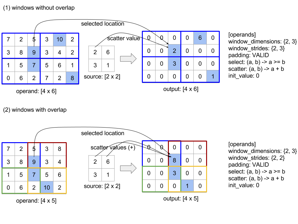
ลำดับการประเมินของฟังก์ชัน scatter เป็นกฎเกณฑ์และอาจไม่ได้มีคำจำกัดความ ดังนั้น ฟังก์ชัน scatter จึงไม่ควรให้ความสำคัญเกินไปกับการเชื่อมโยงใหม่ ดูรายละเอียดเพิ่มเติมได้ที่การสนทนาเกี่ยวกับการเชื่อมโยงในบริบทของ Reduce
ส่ง
ดู XlaBuilder::Send เพิ่มเติม
Send(operand, channel_handle)
| อาร์กิวเมนต์ | ประเภท | อรรถศาสตร์ |
|---|---|---|
operand |
XlaOp |
ข้อมูลที่จะส่ง (อาร์เรย์ประเภท T) |
channel_handle |
ChannelHandle |
ตัวระบุที่ไม่ซ้ำกันสำหรับคู่การส่ง/การรับแต่ละคู่ |
ส่งข้อมูลโอเปอแรนด์ที่ระบุไปยังคำสั่ง Recv ในการคำนวณอื่นที่ใช้แฮนเดิลของช่องเดียวกัน ไม่แสดงข้อมูลใดๆ
เช่นเดียวกับการดำเนินการ Recv ไคลเอ็นต์ API ของการดำเนินการ Send จะแทนการสื่อสารแบบซิงโครนัสและจะถูกแยกย่อยออกเป็นคำสั่ง HLO แบบ 2 แบบ (Send และ SendDone) เพื่อเปิดใช้การโอนข้อมูลแบบไม่พร้อมกัน ดูเพิ่มเติมที่ HloInstruction::CreateSend และ HloInstruction::CreateSendDone
Send(HloInstruction operand, int64 channel_id)
เริ่มการโอนตัวถูกดำเนินการแบบไม่พร้อมกันไปยังทรัพยากรที่จัดสรรโดยคำสั่ง Recv ที่มีรหัสแชแนลเดียวกัน แสดงผลบริบทซึ่งใช้โดยคำสั่ง SendDone ต่อไปนี้เพื่อรอให้การโอนข้อมูลเสร็จสมบูรณ์ บริบทประกอบด้วย {เครื่องหมาย (รูปร่าง), ตัวระบุคำขอ (U32)} และสามารถใช้ได้โดยคำสั่ง SendDone เท่านั้น
SendDone(HloInstruction context)
ต้องรอให้การโอนข้อมูลเสร็จสมบูรณ์เมื่อมีบริบทที่คำสั่ง Send สร้างขึ้น คำสั่งจะไม่แสดงข้อมูลใดๆ
การกำหนดเวลาสำหรับวิธีการของช่อง
คำสั่งดำเนินการของวิธีการ 4 อย่างสำหรับแต่ละช่องทาง (Recv, RecvDone, Send, SendDone) มีดังนี้
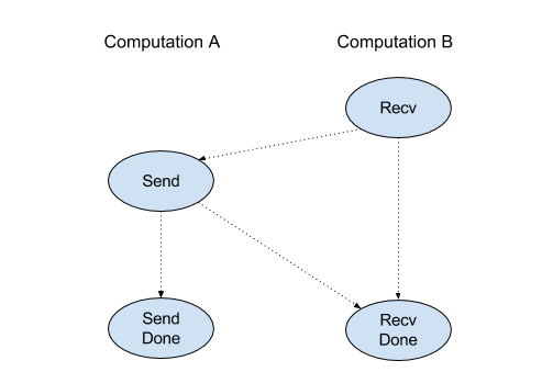
Recvจะเกิดขึ้นก่อนSendSendจะเกิดขึ้นก่อนRecvDoneRecvจะเกิดขึ้นก่อนRecvDoneSendจะเกิดขึ้นก่อนSendDone
เมื่อคอมไพเลอร์แบ็กเอนด์สร้างกำหนดการเชิงเส้นสำหรับการประมวลผลแต่ละรายการที่สื่อสารผ่านคำสั่งแชแนล การประมวลผลนั้นต้องไม่มีรอบ ตัวอย่างเช่น กำหนดการด้านล่างอาจนำไปสู่การติดตาย
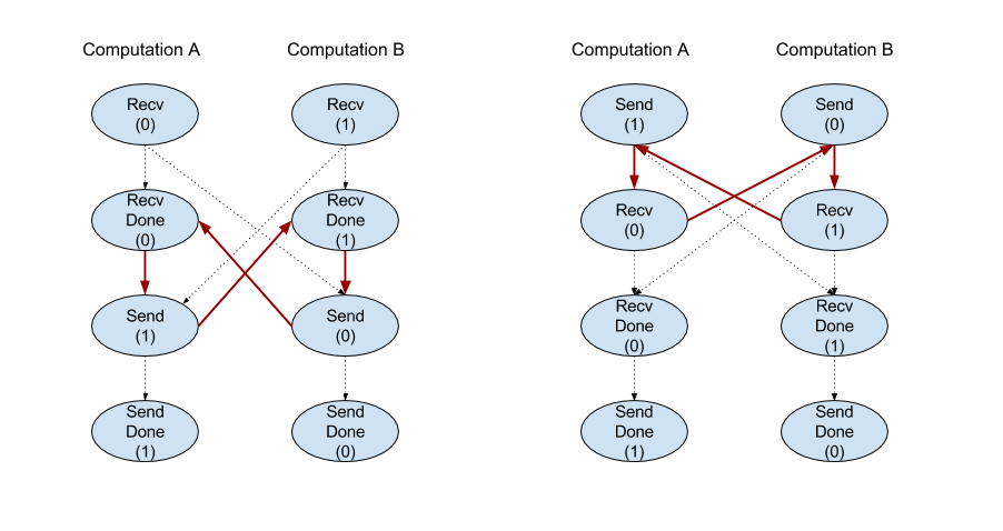
Slice
ดู XlaBuilder::Slice เพิ่มเติม
การแบ่งส่วนจะแยกอาร์เรย์ย่อยจากอาร์เรย์อินพุต อาร์เรย์ย่อยอยู่ในอันดับเดียวกับอินพุต และมีค่าภายในกรอบล้อมรอบภายในอาร์เรย์อินพุตที่ระบุมิติข้อมูลและดัชนีของกรอบล้อมรอบเป็นอาร์กิวเมนต์ของการดำเนินการสไลซ์
Slice(operand, start_indices, limit_indices, strides)
| อาร์กิวเมนต์ | ประเภท | อรรถศาสตร์ |
|---|---|---|
operand |
XlaOp |
อาร์เรย์มิติ N ของประเภท T |
start_indices |
ArraySlice<int64> |
รายการจำนวนเต็ม N ที่มีดัชนีเริ่มต้นของส่วนแบ่งสำหรับแต่ละมิติข้อมูล ค่าต้องมากกว่าหรือเท่ากับ 0 |
limit_indices |
ArraySlice<int64> |
รายการจำนวนเต็ม N ที่มีดัชนีสิ้นสุด (แยกเฉพาะ) ของสไลซ์ของแต่ละมิติข้อมูล แต่ละค่าต้องมากกว่าหรือเท่ากับค่า start_indices ที่เกี่ยวข้องสําหรับมิติข้อมูล และน้อยกว่าหรือเท่ากับขนาดของมิติข้อมูล |
strides |
ArraySlice<int64> |
รายการจำนวนเต็ม N ตัวที่กำหนดอัตราก้าวของอินพุตของส่วน ชิ้นส่วนจะเลือกองค์ประกอบ strides[d] ทุกองค์ประกอบในมิติข้อมูล d |
ตัวอย่าง 1 มิติ:
let a = {0.0, 1.0, 2.0, 3.0, 4.0}
Slice(a, {2}, {4}) produces:
  {2.0, 3.0}
ตัวอย่าง 2 มิติ:
let b =
 { {0.0,  1.0,  2.0},
   {3.0,  4.0,  5.0},
   {6.0,  7.0,  8.0},
   {9.0, 10.0, 11.0} }

Slice(b, {2, 1}, {4, 3}) produces:
  { { 7.0,  8.0},
    {10.0, 11.0} }
จัดเรียง
ดู XlaBuilder::Sort เพิ่มเติม
Sort(operands, comparator, dimension, is_stable)
| อาร์กิวเมนต์ | ประเภท | อรรถศาสตร์ |
|---|---|---|
operands |
ArraySlice<XlaOp> |
ตัวถูกดำเนินการที่จะจัดเรียง |
comparator |
XlaComputation |
การคำนวณของตัวเปรียบเทียบที่จะใช้ |
dimension |
int64 |
มิติข้อมูลที่จะจัดเรียง |
is_stable |
bool |
ควรใช้การจัดเรียงที่เสถียรหรือไม่ |
หากระบุตัวถูกดำเนินการรายการเดียว:
ถ้าตัวถูกดำเนินการเป็น Tensor อันดับ 1 (อาร์เรย์) ผลลัพธ์จะเป็นอาร์เรย์ที่จัดเรียง หากต้องการจัดเรียงอาร์เรย์ตามลำดับจากน้อยไปมาก เครื่องมือเปรียบเทียบควรเปรียบเทียบน้อยกว่า หลังจากจัดเรียงอาร์เรย์อย่างเป็นทางการแล้ว อาร์เรย์จะคงตำแหน่งดัชนีทั้งหมด
i, jที่มีi < jไว้ที่comparator(value[i], value[j]) = comparator(value[j], value[i]) = falseหรือcomparator(value[i], value[j]) = trueหากตัวถูกดำเนินการมีอันดับสูงกว่า ตัวถูกดำเนินการจะได้รับการจัดเรียงตามมิติข้อมูลที่ให้ไว้ เช่น สำหรับ Tensor ระดับ 2 (เมทริกซ์) ค่ามิติข้อมูล
0จะจัดเรียงทุกคอลัมน์อย่างอิสระ และค่ามิติข้อมูล1จะจัดเรียงแต่ละแถวเอง หากไม่ได้ระบุหมายเลขมิติข้อมูล ระบบจะเลือกมิติข้อมูลสุดท้ายโดยค่าเริ่มต้น สำหรับมิติข้อมูลที่มีการจัดเรียง ระบบจะใช้ลำดับการจัดเรียงแบบเดียวกันกับกรณีอันดับที่ 1
หากมีตัวถูกดำเนินการ n > 1 รายการ
ตัวถูกดำเนินการ
nทั้งหมดต้องเป็น Tensor ที่มีขนาดเท่ากัน ประเภทองค์ประกอบ ของ Tensor อาจแตกต่างกันตัวถูกดำเนินการทั้งหมดจะจัดเรียงไว้ด้วยกัน ไม่ใช่แยกทีละรายการ โดยหลักการแล้ว ตัวถูกดำเนินการ จะได้รับการปฏิบัติเสมือนเป็น Tuple เมื่อตรวจสอบว่าจำเป็นต้องสลับองค์ประกอบของตัวถูกดำเนินการแต่ละรายการที่ตำแหน่งดัชนี
iและjหรือไม่ ระบบจะเรียกตัวเปรียบเทียบด้วยพารามิเตอร์สเกลาร์2 * nโดยที่พารามิเตอร์2 * kจะสอดคล้องกับค่าที่ตำแหน่งiจากตัวถูกดำเนินการk-thและพารามิเตอร์2 * k + 1จะสอดคล้องกับค่าที่ตำแหน่งjจากตัวถูกดำเนินการk-thโดยปกติแล้ว เครื่องมือเปรียบเทียบจะเปรียบเทียบพารามิเตอร์2 * kและ2 * k + 1เข้าด้วยกัน และอาจใช้คู่พารามิเตอร์อื่นเป็นตัวตัดค่าเสมอผลลัพธ์ที่ได้คือ Tuple ที่ประกอบด้วยตัวถูกดำเนินการตามลำดับที่จัดเรียง (พร้อมด้วยมิติข้อมูลที่ให้ไว้ตามด้านบน) ตัวถูกดำเนินการ
i-thของ Tuple สอดคล้องกับตัวถูกดำเนินการi-thของการจัดเรียง
เช่น หากมีตัวถูกดำเนินการ 3 รายการ ได้แก่ operand0 = [3, 1], operand1 = [42, 50], operand2 = [-3.0, 1.1] และตัวเปรียบเทียบจะเปรียบเทียบเฉพาะค่าของ operand0 ที่มีน้อยกว่า เอาต์พุตของการจัดเรียงจะเป็น Tuple ([1, 3], [50, 42], [1.1, -3.0])
หากตั้งค่า is_stable เป็น "จริง" การจัดเรียงจะคงที่ กล่าวคือ หากมีองค์ประกอบที่เครื่องมือเปรียบเทียบถือว่าเท่ากัน ลำดับสัมพัทธ์ของค่าที่เท่ากันจะยังคงอยู่ องค์ประกอบ 2 รายการ e1 และ e2 จะมีค่าเท่ากันก็ต่อเมื่อเป็น comparator(e1, e2) = comparator(e2, e1) = false โดยค่าเริ่มต้น is_stable จะตั้งค่าเป็น "เท็จ"
สลับ
โปรดดูการดำเนินการ tf.reshape ด้วย
Transpose(operand)
| อาร์กิวเมนต์ | ประเภท | อรรถศาสตร์ |
|---|---|---|
operand |
XlaOp |
ตัวถูกดำเนินการที่จะสลับสับเปลี่ยน |
permutation |
ArraySlice<int64> |
วิธีจำกัดมิติข้อมูล |
เรียงสับเปลี่ยนมิติข้อมูลตัวถูกดำเนินการด้วยการเรียงสับเปลี่ยนที่กำหนด ดังนั้น ∀ i . 0 ≤ i < rank ⇒ input_dimensions[permutation[i]] = output_dimensions[i]
กรณีนี้เหมือนกับ Reshape(โอเปอแรนด์ การเรียงสับเปลี่ยน การเรียงสับเปลี่ยน(การเรียงสับเปลี่ยน โอเปร่า) รูปร่าง.dimensions)
TriangularSolve
ดู XlaBuilder::TriangularSolve เพิ่มเติม
แก้ระบบสมการเชิงเส้นที่มีค่าสัมประสิทธิ์สามเหลี่ยมล่างหรือบน
ด้วยการแทนค่าไปข้างหน้าหรือถอยหลัง กิจวัตรนี้จะประกาศตามมิติข้อมูลนําทางระบบเมทริกซ์ op(a) * x =
b หรือ x * op(a) = b สําหรับตัวแปร x ที่ระบุ a และ b โดยที่ op(a) เป็น op(a) = a หรือ op(a) = Transpose(a) หรือ op(a) = Conj(Transpose(a))
TriangularSolve(a, b, left_side, lower, unit_diagonal, transpose_a)
| อาร์กิวเมนต์ | ประเภท | อรรถศาสตร์ |
|---|---|---|
a |
XlaOp |
อาร์เรย์อันดับ > 2 ของประเภทเชิงซ้อนหรือจุดลอยตัวที่มีรูปร่าง [..., M, M] |
b |
XlaOp |
อาร์เรย์อันดับ > 2 ประเภทเดียวกันที่มีรูปร่าง [..., M, K] หาก left_side เป็นจริง [..., K, M] ในกรณีอื่นๆ |
left_side |
bool |
ระบุว่าจะแก้ระบบในรูปแบบ op(a) * x = b (true) หรือ x * op(a) = b (false) |
lower |
bool |
จะใช้สามเหลี่ยมบนหรือล่างของ a |
unit_diagonal |
bool |
หาก true จะถือว่าองค์ประกอบแนวทแยงของ a เป็น 1 และไม่มีการเข้าถึง |
transpose_a |
Transpose |
จะใช้ a ตามเดิม สลับสับเปลี่ยนหรือสลับสังยุค |
ข้อมูลที่ป้อนจะอ่านจากสามเหลี่ยมล่าง/บนของ a เท่านั้น โดยขึ้นอยู่กับค่าของ lower และจะไม่สนใจค่าจากสามเหลี่ยมอื่นๆ ข้อมูลเอาต์พุตจะแสดงในสามเหลี่ยมเดียวกัน ค่าในสามเหลี่ยมอีกรูปหนึ่งเป็นตัวกำหนดการใช้งานและอาจเป็นอะไรก็ได้
หากอันดับของ a และ b มากกว่า 2 ระบบจะถือว่ามีกลุ่มของเมทริกซ์ โดยทั้งหมดยกเว้นมิติข้อมูลรอง 2 คือมิติข้อมูลกลุ่ม a และ b ต้องมีมิติข้อมูลกลุ่มเท่าๆ กัน
กระโปรงบัลเลต์
ดู XlaBuilder::Tuple เพิ่มเติม
Tuple ที่มีจำนวนแฮนเดิลข้อมูลตัวแปร แต่ละแฮนเดิลมีรูปร่างของตัวเอง
ค่านี้คล้ายกับ std::tuple ใน C++ โดยหลักการแล้วคือ
let v: f32[10] = f32[10]{0, 1, 2, 3, 4, 5, 6, 7, 8, 9};
let s: s32 = 5;
let t: (f32[10], s32) = tuple(v, s);
สามารถแตกโครงสร้าง (เข้าถึง) ผ่านการดำเนินการ GetTupleElement ได้
ในขณะที่
ดู XlaBuilder::While เพิ่มเติม
While(condition, body, init)
| อาร์กิวเมนต์ | ประเภท | อรรถศาสตร์ |
|---|---|---|
condition |
XlaComputation |
XlaComputation ของประเภท T -> PRED ซึ่งกำหนดเงื่อนไขการสิ้นสุดของลูป |
body |
XlaComputation |
XlaComputation ของประเภท T -> T ซึ่งกำหนดเนื้อหาของลูป |
init |
T |
ค่าเริ่มต้นสำหรับพารามิเตอร์ของ condition และ body |
เรียกใช้ body ตามลำดับจนกระทั่ง condition ล้มเหลว ซึ่งคล้ายกับกรณีทั่วไปที่วนซ้ำในภาษาอื่นๆ หลายภาษา ยกเว้นความแตกต่างและข้อจำกัดที่ระบุไว้ด้านล่าง
- โหนด
Whileแสดงผลค่าประเภทTซึ่งเป็นผลลัพธ์จากการดำเนินการล่าสุดของbody - รูปร่างของประเภท
Tจะกำหนดแบบคงที่และต้องเหมือนกันในทุกการทำซ้ำ
พารามิเตอร์ T ของการคำนวณจะเริ่มด้วยค่า init ในการทำซ้ำครั้งแรก และจะอัปเดตเป็นผลลัพธ์ใหม่โดยอัตโนมัติจาก body ในการทำซ้ำแต่ละครั้ง
กรณีการใช้งานหลักอย่างหนึ่งของโหนด While คือการดำเนินการฝึกซ้ำในโครงข่ายระบบประสาทเทียม ซูโดโค้ดอย่างง่ายจะแสดงที่ด้านล่างพร้อมกับกราฟที่แสดงถึงการคำนวณ ดูโค้ดได้ใน while_test.cc
ประเภท T ในตัวอย่างนี้คือ Tuple ที่ประกอบด้วย int32 สำหรับจำนวนการปรับปรุง และ vector[10] สำหรับ Accumulator สำหรับการทำซ้ำ 1, 000 ครั้ง ลูปจะใส่เวกเตอร์คงที่ลงในแอคคิวมูเลเตอร์เสมอ
// Pseudocode for the computation.
init = {0, zero_vector[10]} // Tuple of int32 and float[10].
result = init;
while (result(0) < 1000) {
  iteration = result(0) + 1;
  new_vector = result(1) + constant_vector[10];
  result = {iteration, new_vector};
}