Phần sau đây mô tả ngữ nghĩa của các thao tác được xác định trong giao diện XlaBuilder. Thông thường, các thao tác này sẽ ánh xạ một với một với các thao tác được xác định trong giao diện RPC trong xla_data.proto.
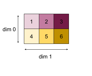
Lưu ý về thuật ngữ: loại dữ liệu khái quát hoá XLA liên quan đến là một mảng N chiều (N-dimensional array) chứa các phần tử thuộc một số loại đồng nhất (chẳng hạn như số thực 32 bit). Trong suốt tài liệu, mảng được dùng để biểu thị một mảng phương diện tuỳ ý. Để thuận tiện, các trường hợp đặc biệt sẽ có tên cụ thể và quen thuộc hơn; ví dụ: vectơ là mảng 1 chiều và ma trận là mảng 2 chiều.
AfterAll
Hãy xem thêm XlaBuilder::AfterAll.
Sau tất cả sẽ lấy một số lượng mã thông báo đa dạng và tạo ra một mã thông báo duy nhất. Mã thông báo là các loại nguyên hàm có thể được tạo luồng giữa các hoạt động có hiệu ứng phụ để thực thi thứ tự. Bạn có thể dùng AfterAll làm mã kết hợp để yêu cầu một toán tử sau một thao tác đã đặt.
AfterAll(operands)
| Đối số | Loại | Ngữ nghĩa |
|---|---|---|
operands |
XlaOp |
số lượng mã thông báo biến thiên |
AllGather
Hãy xem thêm XlaBuilder::AllGather.
Thực hiện việc nối các bản sao.
AllGather(operand, all_gather_dim, shard_count, replica_group_ids,
channel_id)
| Đối số | Loại | Ngữ nghĩa |
|---|---|---|
operand
|
XlaOp
|
Mảng để nối trên các bản sao |
all_gather_dim |
int64 |
Phương diện nối |
replica_groups
|
vectơ của các vectơ của int64 |
Các nhóm thực hiện việc nối |
channel_id
|
int64 không bắt buộc
|
Mã nhận dạng kênh không bắt buộc để giao tiếp nhiều mô-đun |
replica_groupslà danh sách các nhóm bản sao dùng để thực hiện việc nối (bạn có thể truy xuất mã bản sao của bản sao hiện tại bằng cách sử dụngReplicaId). Thứ tự của các bản sao trong mỗi nhóm sẽ xác định thứ tự chứa dữ liệu đầu vào của các bản sao đó trong kết quả.replica_groupsphải trống (trong trường hợp đó, mọi bản sao thuộc về một nhóm duy nhất, được sắp xếp theo thứ tự từ0đếnN - 1) hoặc chứa cùng số phần tử với số lượng bản sao. Ví dụ:replica_groups = {0, 2}, {1, 3}thực hiện việc nối giữa các bản sao0với2, cũng như1và3.shard_countlà kích thước của mỗi nhóm bản sao. Chúng ta cần điều này trong trường hợpreplica_groupstrống.channel_idđược dùng để giao tiếp trên nhiều mô-đun: chỉ các thao tácall-gathercó cùngchannel_idmới có thể giao tiếp với nhau.
Hình dạng đầu ra là hình dạng đầu vào với all_gather_dim có kích thước lớn hơn shard_count lần. Ví dụ: nếu có 2 bản sao và toán hạng có giá trị [1.0, 2.5] và [3.0, 5.25] tương ứng trên 2 bản sao, thì giá trị đầu ra từ op này, trong đó all_gather_dim là 0 sẽ là [1.0, 2.5, 3.0,
5.25] trên cả hai bản sao.
AllReduce
Hãy xem thêm XlaBuilder::AllReduce.
Thực hiện phép tính tuỳ chỉnh trên các bản sao.
AllReduce(operand, computation, replica_group_ids, channel_id)
| Đối số | Loại | Ngữ nghĩa |
|---|---|---|
operand
|
XlaOp
|
Mảng hoặc một bộ dữ liệu không trống gồm các mảng để giảm thiểu trên các bản sao |
computation |
XlaComputation |
Tính toán rút gọn |
replica_groups
|
vectơ của các vectơ của int64 |
Các nhóm thực hiện rút gọn |
channel_id
|
int64 không bắt buộc
|
Mã nhận dạng kênh không bắt buộc để giao tiếp nhiều mô-đun |
- Khi
operandlà một bộ dữ liệu của mảng, việc giảm tất cả sẽ được thực hiện trên từng phần tử của bộ dữ liệu. replica_groupslà danh sách các nhóm bản sao được thực hiện trong quá trình rút gọn (mã bản sao của bản sao hiện tại có thể được truy xuất bằngReplicaId).replica_groupsphải để trống (trong trường hợp đó, tất cả các bản sao đều thuộc một nhóm) hoặc chứa cùng số lượng phần tử với số lượng bản sao. Ví dụ:replica_groups = {0, 2}, {1, 3}thực hiện giảm thiểu giữa các bản sao0và2, cũng như1và3.channel_idđược dùng để giao tiếp trên nhiều mô-đun: chỉ các thao tácall-reducecó cùngchannel_idmới có thể giao tiếp với nhau.
Hình dạng đầu ra giống với hình dạng đầu vào. Ví dụ: nếu có 2 bản sao và toán hạng có giá trị [1.0, 2.5] và [3.0, 5.25] tương ứng trên 2 bản sao, thì giá trị đầu ra của phép tính tổng hợp và vận hành này sẽ là [4.0, 7.75] trên cả hai bản sao. Nếu dữ liệu đầu vào là một bộ dữ liệu, thì dữ liệu đầu ra cũng sẽ là một bộ dữ liệu.
Việc tính toán kết quả của AllReduce cần có một dữ liệu đầu vào từ mỗi bản sao. Vì vậy, nếu một bản sao thực thi một nút AllReduce nhiều lần hơn một bản sao khác, thì bản sao cũ sẽ đợi vĩnh viễn. Vì các bản sao đều đang chạy cùng một chương trình, nên không có nhiều cách để điều đó xảy ra. Tuy nhiên, có thể xảy ra khi điều kiện của vòng lặp while phụ thuộc vào dữ liệu từ nguồn cấp dữ liệu và dữ liệu được truyền khiến vòng lặp while lặp lại nhiều lần trên một bản sao hơn so với bản sao khác.
AllToAll
Hãy xem thêm XlaBuilder::AllToAll.
AllToAll là một hoạt động tập hợp gửi dữ liệu từ tất cả các lõi đến tất cả các lõi. Quy trình này có 2 giai đoạn:
- Giai đoạn tán xạ. Trên mỗi lõi, toán hạng được chia thành số khối
split_countdọc theosplit_dimensionsvà các khối được phân tán đến tất cả các lõi, ví dụ: khối thứ i được gửi đến lõi thứ i. - Giai đoạn thu thập. Mỗi lõi sẽ nối các khối đã nhận với
concat_dimension.
Các lõi tham gia có thể được định cấu hình bằng cách:
replica_groups: mỗi ReplicaGroup chứa một danh sách các mã nhận dạng bản sao tham gia vào việc tính toán (mã bản sao của bản sao hiện tại có thể được truy xuất bằngReplicaId). AllToAll sẽ được áp dụng trong các nhóm con theo thứ tự đã chỉ định. Ví dụ:replica_groups = { {1,2,3}, {4,5,0} }có nghĩa là AllToAll sẽ được áp dụng trong các bản sao{1, 2, 3}và trong giai đoạn thu thập, đồng thời các khối đã nhận sẽ được nối theo cùng thứ tự 1, 2, 3. Sau đó, một AllToAll khác sẽ được áp dụng trong các bản sao 4, 5, 0 và thứ tự nối cũng là 4, 5, 0. Nếureplica_groupstrống, tất cả các bản sao đều thuộc về một nhóm, theo thứ tự nối xuất hiện của các bản sao đó.
Điều kiện tiên quyết:
- Kích thước kích thước của toán hạng trên
split_dimensioncó thể chia hết chosplit_count. - Hình dạng của toán hạng không phải là bộ dữ liệu.
AllToAll(operand, split_dimension, concat_dimension, split_count,
replica_groups)
| Đối số | Loại | Ngữ nghĩa |
|---|---|---|
operand |
XlaOp |
mảng đầu vào thứ n |
split_dimension
|
int64
|
Một giá trị trong khoảng [0,
n) đặt tên cho nhóm mà theo đó toán hạng được phân tách |
concat_dimension
|
int64
|
Một giá trị trong khoảng [0,
n) đặt tên cho chiều mà các khối phân tách được nối với nhau |
split_count
|
int64
|
Số lượng lõi tham gia hoạt động này. Nếu replica_groups trống, thì đó phải là số lượng bản sao; nếu không, giá trị này phải bằng số lượng bản sao trong mỗi nhóm. |
replica_groups
|
Vectơ ReplicaGroup
|
Mỗi nhóm chứa một danh sách các mã bản sao. |
Dưới đây là một ví dụ về Alltoall.
XlaBuilder b("alltoall");
auto x = Parameter(&b, 0, ShapeUtil::MakeShape(F32, {4, 16}), "x");
AllToAll(x, /*split_dimension=*/1, /*concat_dimension=*/0, /*split_count=*/4);
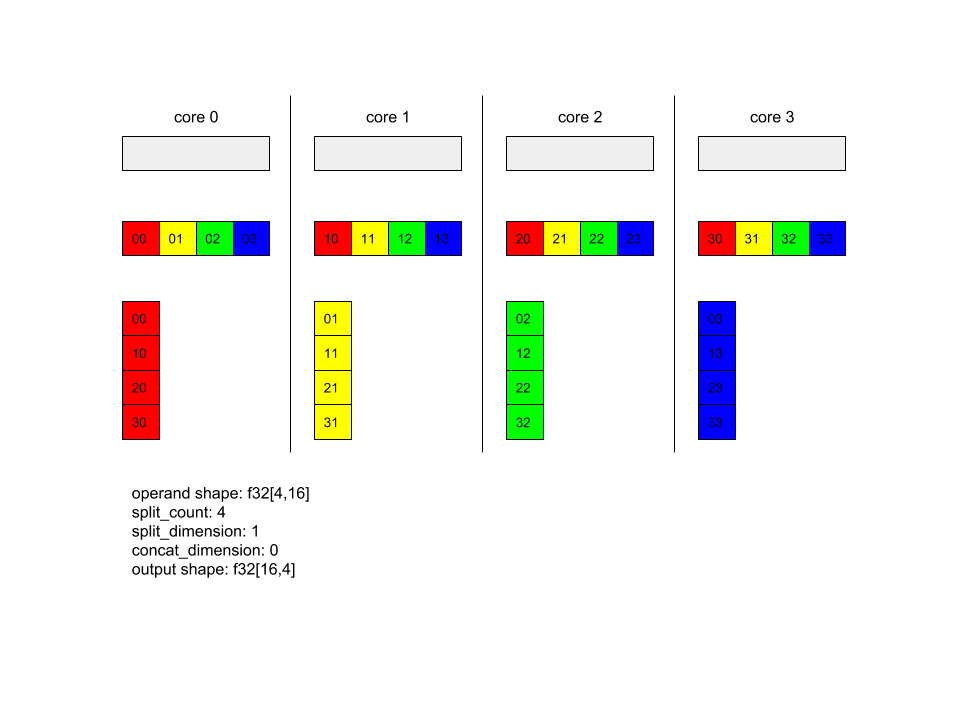
Trong ví dụ này, có 4 lõi tham gia vào Alltoall. Trên mỗi lõi, toán hạng được chia thành 4 phần dọc theo chiều 0, vì vậy mỗi phần có hình dạng f32[4,4]. 4 phần này nằm rải rác đến tất cả các lõi. Sau đó, mỗi lõi nối các phần đã nhận dọc theo chiều 1, theo thứ tự lõi 0-4. Vì vậy, đầu ra trên mỗi lõi có hình dạng f32[16,4].
BatchNormGrad
Ngoài ra, hãy xem XlaBuilder::BatchNormGrad và tài liệu chuẩn hoá lô ban đầu để biết nội dung mô tả chi tiết về thuật toán.
Tính toán độ dốc của tiêu chuẩn lô.
BatchNormGrad(operand, scale, mean, variance, grad_output, epsilon, feature_index)
| Đối số | Loại | Ngữ nghĩa |
|---|---|---|
operand |
XlaOp |
n mảng phương diện cần được chuẩn hoá (x) |
scale |
XlaOp |
Mảng 1 phương diện (\(\gamma\)) |
mean |
XlaOp |
Mảng 1 phương diện (\(\mu\)) |
variance |
XlaOp |
Mảng 1 phương diện (\(\sigma^2\)) |
grad_output |
XlaOp |
Đã chuyển màu cho BatchNormTraining (\(\nabla y\)) |
epsilon |
float |
Giá trị Epsilon (\(\epsilon\)) |
feature_index |
int64 |
Chỉ mục để làm nổi bật phương diện trong operand |
Đối với mỗi tính năng trong phương diện tính năng (feature_index là chỉ mục cho phương diện tính năng trong operand), thao tác này sẽ tính toán độ chuyển màu tương ứng với operand, offset và scale trên tất cả các phương diện khác. feature_index phải là một chỉ mục hợp lệ cho phương diện tính năng trong operand.
Ba độ dốc được xác định bằng các công thức sau (giả sử một mảng 4 chiều là operand và có chỉ mục kích thước tính năng l, kích thước lô m cũng như kích thước không gian w và h):
\[ \begin{split} c_l&= \frac{1}{mwh}\sum_{i=1}^m\sum_{j=1}^w\sum_{k=1}^h \left( \nabla y_{ijkl} \frac{x_{ijkl} - \mu_l}{\sigma^2_l+\epsilon} \right) \\\\ d_l&= \frac{1}{mwh}\sum_{i=1}^m\sum_{j=1}^w\sum_{k=1}^h \nabla y_{ijkl} \\\\ \nabla x_{ijkl} &= \frac{\gamma_{l} }{\sqrt{\sigma^2_{l}+\epsilon} } \left( \nabla y_{ijkl} - d_l - c_l (x_{ijkl} - \mu_{l}) \right) \\\\ \nabla \gamma_l &= \sum_{i=1}^m\sum_{j=1}^w\sum_{k=1}^h \left( \nabla y_{ijkl} \frac{x_{ijkl} - \mu_l}{\sqrt{\sigma^2_{l}+\epsilon} } \right) \\\\\ \nabla \beta_l &= \sum_{i=1}^m\sum_{j=1}^w\sum_{k=1}^h \nabla y_{ijkl} \end{split} \]
Dữ liệu đầu vào mean và variance biểu thị các giá trị khoảnh khắc trên các phương diện theo lô và không gian.
Loại đầu ra là một bộ dữ liệu gồm 3 ô điều khiển:
| Kết quả đầu ra | Loại | Ngữ nghĩa |
|---|---|---|
grad_operand
|
XlaOp
|
độ dốc tương ứng với dữ liệu đầu vào operand ($\nabla x$) |
grad_scale
|
XlaOp
|
độ dốc tương ứng với dữ liệu đầu vào scale ($\nabla
\gamma$) |
grad_offset
|
XlaOp
|
độ dốc tương ứng với dữ liệu đầu vào offset($\nabla
\beta$) |
BatchNormInference
Ngoài ra, hãy xem XlaBuilder::BatchNormInference và tài liệu chuẩn hoá lô ban đầu để biết nội dung mô tả chi tiết về thuật toán.
Chuẩn hoá một mảng trên các kích thước theo lô và không gian.
BatchNormInference(operand, scale, offset, mean, variance, epsilon, feature_index)
| Đối số | Loại | Ngữ nghĩa |
|---|---|---|
operand |
XlaOp |
n mảng thứ nguyên cần được chuẩn hoá |
scale |
XlaOp |
Mảng 1 phương diện |
offset |
XlaOp |
Mảng 1 phương diện |
mean |
XlaOp |
Mảng 1 phương diện |
variance |
XlaOp |
Mảng 1 phương diện |
epsilon |
float |
Giá trị epsilon |
feature_index |
int64 |
Chỉ mục để làm nổi bật phương diện trong operand |
Đối với mỗi tính năng trong phương diện tính năng (feature_index là chỉ mục cho phương diện tính năng trong operand), phép toán này sẽ tính giá trị trung bình và phương sai trên tất cả các phương diện khác, đồng thời sử dụng giá trị trung bình và phương sai để chuẩn hoá từng phần tử trong operand. feature_index phải là một chỉ mục hợp lệ cho nhóm tính năng trong operand.
BatchNormInference tương đương với việc gọi BatchNormTraining mà không tính toán mean và variance cho từng lô. Phương thức này sử dụng dữ liệu đầu vào mean và variance dưới dạng giá trị ước tính. Mục đích của thao tác này là giảm độ trễ trong suy luận, do đó có tên là BatchNormInference.
Đầu ra là một mảng n chiều được chuẩn hoá có hình dạng giống như đầu vào operand.
BatchNormTraining
Hãy xem thêm XlaBuilder::BatchNormTraining và the original batch normalization paper để biết nội dung mô tả chi tiết về thuật toán.
Chuẩn hoá một mảng trên các kích thước theo lô và không gian.
BatchNormTraining(operand, scale, offset, epsilon, feature_index)
| Đối số | Loại | Ngữ nghĩa |
|---|---|---|
operand |
XlaOp |
n mảng phương diện cần được chuẩn hoá (x) |
scale |
XlaOp |
Mảng 1 phương diện (\(\gamma\)) |
offset |
XlaOp |
Mảng 1 phương diện (\(\beta\)) |
epsilon |
float |
Giá trị Epsilon (\(\epsilon\)) |
feature_index |
int64 |
Chỉ mục để làm nổi bật phương diện trong operand |
Đối với mỗi tính năng trong phương diện tính năng (feature_index là chỉ mục cho phương diện tính năng trong operand), phép toán này sẽ tính giá trị trung bình và phương sai trên tất cả các phương diện khác, đồng thời sử dụng giá trị trung bình và phương sai để chuẩn hoá từng phần tử trong operand. feature_index phải là một chỉ mục hợp lệ cho nhóm tính năng trong operand.
Thuật toán diễn ra như sau đối với mỗi lô trong operand \(x\) chứa các phần tử m với w và h là kích thước của các kích thước không gian (giả sử operand là một mảng 4 chiều):
Tính toán giá trị trung bình theo lô \(\mu_l\) cho mỗi tính năng
ltrong kích thước tính năng:\(\mu_l=\frac{1}{mwh}\sum_{i=1}^m\sum_{j=1}^w\sum_{k=1}^h x_{ijkl}\)Tính toán phương sai của lô \(\sigma^2_l\): $\sigma^2l=\frac{1}{mWH}\sum{i=1}^m\sum{j=1}^w\sum{k=1}^h (x_{ijkl} - \mu_l)^2$
Chuẩn hoá, điều chỉnh theo tỷ lệ và thay đổi: \(y_{ijkl}=\frac{\gamma_l(x_{ijkl}-\mu_l)}{\sqrt[2]{\sigma^2_l+\epsilon} }+\beta_l\)
Giá trị epsilon (thường là một số nhỏ) được thêm vào để tránh lỗi chia cho 0.
Loại đầu ra là một bộ dữ liệu gồm ba XlaOp:
| Kết quả đầu ra | Loại | Ngữ nghĩa |
|---|---|---|
output
|
XlaOp
|
mảng thứ nguyên n có cùng hình dạng với dữ liệu đầu vào operand (y) |
batch_mean |
XlaOp |
Mảng 1 phương diện (\(\mu\)) |
batch_var |
XlaOp |
Mảng 1 phương diện (\(\sigma^2\)) |
batch_mean và batch_var là các khoảnh khắc được tính toán trên các kích thước lô và kích thước không gian bằng các công thức ở trên.
BitcastConvertType
Hãy xem thêm XlaBuilder::BitcastConvertType.
Tương tự như một tf.bitcast trong TensorFlow, thực hiện một thao tác truyền bit liên quan đến phần tử, từ hình dạng dữ liệu đến hình dạng mục tiêu. Kích thước đầu vào và đầu ra phải khớp nhau, ví dụ: các phần tử s32 trở thành phần tử f32 thông qua quy trình bitcast và một phần tử s32 sẽ trở thành bốn phần tử s8. Bitcast được triển khai dưới dạng truyền cấp thấp, vì vậy, các máy có các cách biểu diễn dấu phẩy động khác nhau sẽ cho kết quả khác nhau.
BitcastConvertType(operand, new_element_type)
| Đối số | Loại | Ngữ nghĩa |
|---|---|---|
operand |
XlaOp |
mảng loại T có mờ D |
new_element_type |
PrimitiveType |
loại U |
Kích thước của toán hạng và hình dạng mục tiêu phải khớp nhau, ngoài kích thước cuối cùng sẽ thay đổi theo tỷ lệ kích thước gốc trước và sau khi chuyển đổi.
Loại thành phần nguồn và đích không được là bộ giá trị.
Bitcast chuyển đổi sang kiểu gốc có chiều rộng khác
Lệnh HLO BitcastConvert hỗ trợ trường hợp kích thước của loại phần tử đầu ra T' không bằng kích thước của phần tử đầu vào T. Về mặt lý thuyết, toàn bộ thao tác là một phương thức bit và không thay đổi byte cơ bản, nên hình dạng của phần tử đầu ra sẽ phải thay đổi. Đối với B = sizeof(T), B' =
sizeof(T'), có hai trường hợp có thể xảy ra.
Trước tiên, khi B > B', hình dạng đầu ra sẽ có kích thước nhỏ nhất là B/B'. Ví dụ:
f16[10,2]{1,0} %output = f16[10,2]{1,0} bitcast-convert(f32[10]{0} %input)
Quy tắc này giữ nguyên đối với những đại lượng vô hướng hiệu lực:
f16[2]{0} %output = f16[2]{0} bitcast-convert(f32[] %input)
Ngoài ra, đối với B' > B, lệnh yêu cầu chiều logic cuối cùng của hình dạng nhập phải bằng B'/B và chiều này sẽ bị loại bỏ trong quá trình chuyển đổi:
f32[10]{0} %output = f32[10]{0} bitcast-convert(f16[10,2]{1,0} %input)
Lưu ý rằng việc chuyển đổi giữa các bitwidth khác nhau không theo nguyên tố.
Truyền
Hãy xem thêm XlaBuilder::Broadcast.
Thêm phương diện vào một mảng bằng cách sao chép dữ liệu trong mảng đó.
Broadcast(operand, broadcast_sizes)
| Đối số | Loại | Ngữ nghĩa |
|---|---|---|
operand |
XlaOp |
Mảng cần sao chép |
broadcast_sizes |
ArraySlice<int64> |
Kích thước của các phương diện mới |
Các kích thước mới được chèn vào bên trái, tức là nếu broadcast_sizes có giá trị {a0, ..., aN} và hình dạng toán hạng có kích thước {b0, ..., bM} thì hình dạng đầu ra có kích thước {a0, ..., aN, b0, ..., bM}.
Việc lập chỉ mục phương diện mới thành các bản sao của toán hạng, tức là
output[i0, ..., iN, j0, ..., jM] = operand[j0, ..., jM]
Ví dụ: nếu operand là f32 vô hướng có giá trị 2.0f và broadcast_sizes là {2, 3}, thì kết quả sẽ là một mảng có hình dạng f32[2, 3] và tất cả giá trị trong kết quả sẽ là 2.0f.
BroadcastInDim
Hãy xem thêm XlaBuilder::BroadcastInDim.
Mở rộng kích thước và thứ hạng của một mảng bằng cách sao chép dữ liệu trong mảng.
BroadcastInDim(operand, out_dim_size, broadcast_dimensions)
| Đối số | Loại | Ngữ nghĩa |
|---|---|---|
operand |
XlaOp |
Mảng cần sao chép |
out_dim_size |
ArraySlice<int64> |
Kích thước của kích thước của hình dạng mục tiêu |
broadcast_dimensions |
ArraySlice<int64> |
Kích thước nào trong hình dạng mục tiêu, mỗi chiều của hình dạng toán hạng tương ứng với |
Tương tự như Broadcast, nhưng cho phép thêm kích thước ở bất kỳ đâu và mở rộng các kích thước hiện có với kích thước 1.
operand được truyền tin đến hình dạng được out_dim_size mô tả.
broadcast_dimensions ánh xạ các kích thước của operand đến kích thước của hình dạng mục tiêu, tức là chiều thứ i của toán hạng được ánh xạ tới kích thước broadcast_dimension[i] của hình dạng đầu ra. Kích thước của operand phải có kích thước 1 hoặc có cùng kích thước với kích thước trong hình dạng đầu ra mà chúng được ánh xạ đến. Các kích thước còn lại được điền bằng các tham số có kích thước 1. Sau đó, truyền phát theo phương diện thoái hoá sẽ truyền dọc theo các phương diện thoái hoá này để đạt được hình dạng đầu ra. Ngữ nghĩa được mô tả chi tiết trên trang thông báo.
Gọi
Hãy xem thêm XlaBuilder::Call.
Gọi một phép tính với các đối số đã cho.
Call(computation, args...)
| Đối số | Loại | Ngữ nghĩa |
|---|---|---|
computation |
XlaComputation |
tính toán kiểu T_0, T_1, ..., T_{N-1} -> S với N tham số thuộc kiểu tuỳ ý |
args |
chuỗi N XlaOp giây |
N đối số thuộc kiểu tuỳ ý |
Tính chất và loại của args phải khớp với các tham số của computation. Không được phép không có args.
Cholesky
Hãy xem thêm XlaBuilder::Cholesky.
Tính toán quá trình phân ly Cholesky của một loạt ma trận xác định dương đối xứng (Hermitian).
Cholesky(a, lower)
| Đối số | Loại | Ngữ nghĩa |
|---|---|---|
a |
XlaOp |
một hạng > 2 mảng của một kiểu dấu phẩy động hoặc phức tạp. |
lower |
bool |
liệu sử dụng tam giác trên hay tam giác dưới của a. |
Nếu lower là true, tính toán ma trận tam giác thấp hơn l sao cho $a = l .
l^T$. Nếu lower là false, tính toán ma trận tam giác trên u sao cho\(a = u^T . u\).
Dữ liệu đầu vào chỉ được đọc từ tam giác dưới/trên của a, tuỳ thuộc vào giá trị của lower. Các giá trị từ tam giác khác sẽ bị bỏ qua. Dữ liệu đầu ra được trả về trong cùng một tam giác; các giá trị trong tam giác khác được xác định theo phương thức triển khai và có thể là bất kỳ giá trị nào.
Nếu thứ hạng của a lớn hơn 2, thì a được coi là một lô ma trận, trong đó tất cả ngoại trừ 2 kích thước nhỏ đều là kích thước lô.
Nếu a không phải là xác định dương đối xứng (Hermitian), kết quả sẽ được xác định dựa trên phương thức triển khai.
Kẹp
Hãy xem thêm XlaBuilder::Clamp.
Gắn một toán hạng trong phạm vi từ giá trị tối thiểu đến tối đa.
Clamp(min, operand, max)
| Đối số | Loại | Ngữ nghĩa |
|---|---|---|
min |
XlaOp |
mảng loại T |
operand |
XlaOp |
mảng loại T |
max |
XlaOp |
mảng loại T |
Cho sẵn một toán hạng cũng như các giá trị tối thiểu và tối đa, trả về toán hạng nếu nằm trong khoảng từ giá trị tối thiểu đến tối đa, nếu không sẽ trả về giá trị tối thiểu nếu toán hạng nằm dưới phạm vi này hoặc giá trị lớn nhất nếu toán hạng nằm trên phạm vi này. Tức là clamp(a, x, b) = min(max(a, x), b).
Cả 3 mảng phải có cùng hình dạng. Ngoài ra, ở dạng thông báo truyền tin hạn chế, min và/hoặc max có thể là đại lượng vô hướng thuộc kiểu T.
Ví dụ với min và max vô hướng:
let operand: s32[3] = {-1, 5, 9};
let min: s32 = 0;
let max: s32 = 6;
==>
Clamp(min, operand, max) = s32[3]{0, 5, 6};
Thu gọn
Hãy xem thêm XlaBuilder::Collapse và toán tử tf.reshape.
Thu gọn các phương diện của một mảng thành một phương diện.
Collapse(operand, dimensions)
| Đối số | Loại | Ngữ nghĩa |
|---|---|---|
operand |
XlaOp |
mảng loại T |
dimensions |
Vectơ int64 |
tập con liên tiếp, theo thứ tự của các tham số T. |
Thao tác thu gọn sẽ thay thế tập hợp con các phương diện của toán hạng đã cho bằng một phương diện duy nhất. Các đối số đầu vào là một mảng loại T tuỳ ý và vectơ hằng số tại thời gian biên dịch của các chỉ mục kích thước. Các chỉ mục kích thước phải là một thứ tự (số kích thước từ thấp đến cao), tập hợp con liên tiếp của các tham số T. Do đó, {0, 1, 2}, {0, 1} hoặc {1, 2} đều là các tập hợp phương diện hợp lệ, nhưng {1, 0} hoặc {0, 2} thì không. Các kích thước này được thay thế bằng một phương diện mới duy nhất, ở cùng vị trí trong trình tự phương diện khi các phương diện đó thay thế, với kích thước phương diện mới bằng với tích của kích thước kích thước ban đầu. Số phương diện thấp nhất trong dimensions là phương diện có tốc độ thay đổi chậm nhất (chính nhất) trong vòng lặp lồng nhau, thu gọn các phương diện này, và số kích thước cao nhất sẽ thay đổi nhanh nhất (hầu hết nhỏ nhất). Hãy xem toán tử tf.reshape nếu cần thêm thứ tự thu gọn chung.
Ví dụ: giả sử v là một mảng gồm 24 phần tử:
let v = f32[4x2x3] { { {10, 11, 12},  {15, 16, 17} },
{ {20, 21, 22},  {25, 26, 27} },
{ {30, 31, 32},  {35, 36, 37} },
{ {40, 41, 42},  {45, 46, 47} } };

// Collapse to a single dimension, leaving one dimension.
let v012 = Collapse(v, {0,1,2});
then v012 == f32[24] {10, 11, 12, 15, 16, 17,
20, 21, 22, 25, 26, 27,
30, 31, 32, 35, 36, 37,
40, 41, 42, 45, 46, 47};

// Collapse the two lower dimensions, leaving two dimensions.
let v01 = Collapse(v, {0,1});
then v01 == f32[4x6] { {10, 11, 12, 15, 16, 17},
{20, 21, 22, 25, 26, 27},
{30, 31, 32, 35, 36, 37},
{40, 41, 42, 45, 46, 47} };

// Collapse the two higher dimensions, leaving two dimensions.
let v12 = Collapse(v, {1,2});
then v12 == f32[8x3] { {10, 11, 12},
{15, 16, 17},
{20, 21, 22},
{25, 26, 27},
{30, 31, 32},
{35, 36, 37},
{40, 41, 42},
{45, 46, 47} };
CollectivePermute
Hãy xem thêm XlaBuilder::CollectivePermute.
CollectivePermute là một toán tử tập thể sẽ gửi và nhận các bản sao của dữ liệu trên nhiều nền tảng.
CollectivePermute(operand, source_target_pairs)
| Đối số | Loại | Ngữ nghĩa |
|---|---|---|
operand |
XlaOp |
mảng đầu vào thứ n |
source_target_pairs |
Vectơ <int64, int64> |
Danh sách các cặp (source_replica_id, target_replica_id). Đối với mỗi cặp, toán hạng được gửi từ bản sao nguồn đến bản sao đích. |
Lưu ý rằng source_target_pair có các hạn chế sau:
- Hai cặp bất kỳ không được có cùng một mã nhận dạng bản sao mục tiêu và không được có cùng một mã bản sao nguồn.
- Nếu mã bản sao không phải là mục tiêu trong bất kỳ cặp nào, thì đầu ra trên bản sao đó là một tensor bao gồm 0(các) có cùng hình dạng với đầu vào.
Nối
Hãy xem thêm XlaBuilder::ConcatInDim.
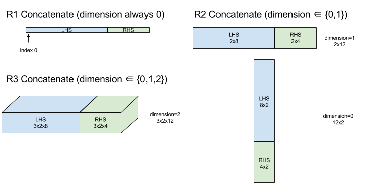
Phép nối sẽ tạo một mảng từ nhiều toán hạng mảng. Mảng có cùng thứ hạng với mỗi toán hạng mảng đầu vào (phải cùng hạng với nhau) và chứa các đối số theo thứ tự đã được chỉ định.
Concatenate(operands..., dimension)
| Đối số | Loại | Ngữ nghĩa |
|---|---|---|
operands |
chuỗi N XlaOp |
N mảng loại T có kích thước [L0, L1, ...]. Yêu cầu N >= 1. |
dimension |
int64 |
Một giá trị trong khoảng [0, N) đặt tên cho phương diện cần liên kết giữa operands. |
Ngoại trừ dimension, tất cả phương diện phải giống nhau. Điều này là do XLA không hỗ trợ các mảng "xuất hiện trên màn hình". Ngoài ra, xin lưu ý rằng bạn không thể nối các giá trị hạng-0 (vì không thể đặt tên cho kích thước xảy ra quá trình nối).
Ví dụ về 1 phương diện:
Concat({ {2, 3}, {4, 5}, {6, 7} }, 0)
>>> {2, 3, 4, 5, 6, 7}
Ví dụ về 2 chiều:
let a = {
{1, 2},
{3, 4},
{5, 6},
};
let b = {
{7, 8},
};
Concat({a, b}, 0)
>>> {
{1, 2},
{3, 4},
{5, 6},
{7, 8},
}
Biểu đồ:
Câu lệnh có điều kiện
Hãy xem thêm XlaBuilder::Conditional.
Conditional(pred, true_operand, true_computation, false_operand,
false_computation)
| Đối số | Loại | Ngữ nghĩa |
|---|---|---|
pred |
XlaOp |
Giá trị vô hướng của kiểu PRED |
true_operand |
XlaOp |
Đối số thuộc loại \(T_0\) |
true_computation |
XlaComputation |
Tính năng XlaComputation thuộc loại \(T_0 \to S\) |
false_operand |
XlaOp |
Đối số thuộc loại \(T_1\) |
false_computation |
XlaComputation |
Tính năng XlaComputation thuộc loại \(T_1 \to S\) |
Thực thi true_computation nếu pred là true, false_computation nếu pred là false, và trả về kết quả.
true_computation phải nhận một đối số duy nhất thuộc loại \(T_0\) và sẽ
được gọi bằng true_operand phải cùng loại. false_computation phải nhận một đối số duy nhất thuộc loại \(T_1\) và sẽ được gọi bằng false_operand. Đối số này phải cùng loại. Loại giá trị được trả về của true_computation và false_computation phải giống nhau.
Xin lưu ý rằng chỉ một trong số true_computation và false_computation sẽ được thực thi tuỳ thuộc vào giá trị của pred.
Conditional(branch_index, branch_computations, branch_operands)
| Đối số | Loại | Ngữ nghĩa |
|---|---|---|
branch_index |
XlaOp |
Giá trị vô hướng của kiểu S32 |
branch_computations |
chuỗi N XlaComputation |
Phép tính toán học thuộc loại \(T_0 \to S , T_1 \to S , ..., T_{N-1} \to S\) |
branch_operands |
chuỗi N XlaOp |
Đối số thuộc kiểu \(T_0 , T_1 , ..., T_{N-1}\) |
Thực thi branch_computations[branch_index] và trả về kết quả. Nếu branch_index là một S32 < 0 hoặc >= N, thì branch_computations[N-1] sẽ được thực thi dưới dạng nhánh mặc định.
Mỗi branch_computations[b] phải nhận một đối số duy nhất thuộc loại \(T_b\) và
sẽ được gọi bằng branch_operands[b] phải cùng loại. Loại giá trị trả về của mỗi branch_computations[b] phải giống nhau.
Xin lưu ý rằng chỉ một trong các branch_computations sẽ được thực thi tuỳ thuộc vào giá trị của branch_index.
Lượt chuyển đổi (kết hợp)
Hãy xem thêm XlaBuilder::Conv.
Là ConvWithGeneralPadding, nhưng khoảng đệm được chỉ định theo cách ngắn gọn là SAME hoặc hợp lệ. Tương tự khoảng đệm cho đầu vào (lhs) bằng các số 0 để đầu ra có hình dạng giống với đầu vào khi không tính đến. Khoảng đệm KHÔNG HỢP LỆ đơn giản có nghĩa là không có khoảng đệm.
ConvWithGeneralPadding (tích chập)
Hãy xem thêm XlaBuilder::ConvWithGeneralPadding.
Tính toán tích chập của kiểu dùng trong mạng nơron. Ở đây, tích chập có thể được coi là một cửa sổ n chiều di chuyển qua vùng cơ sở n chiều và phép tính được thực hiện cho từng vị trí có thể có của cửa sổ.
| Đối số | Loại | Ngữ nghĩa |
|---|---|---|
lhs |
XlaOp |
xếp hạng n+2 mảng đầu vào |
rhs |
XlaOp |
hạng n+2 mảng trọng số hạt nhân |
window_strides |
ArraySlice<int64> |
mảng n-d của sải hạt nhân |
padding |
ArraySlice< pair<int64,int64>> |
Mảng n-d khoảng đệm (thấp, cao) |
lhs_dilation |
ArraySlice<int64> |
Mảng hệ số giãn nở n-d lhs |
rhs_dilation |
ArraySlice<int64> |
Mảng hệ số giãn nở n-d rhs |
feature_group_count |
int64 | số lượng nhóm tính năng |
batch_group_count |
int64 | số lượng nhóm lô |
n là số lượng kích thước không gian. Đối số lhs là một mảng xếp hạng n+2 mô tả vùng cơ sở. Đây được gọi là dữ liệu đầu vào, mặc dù tất nhiên rhs cũng là dữ liệu đầu vào. Trong mạng nơron, đây là những hoạt động kích hoạt dữ liệu đầu vào.
Các chiều n+2 theo thứ tự sau:
batch: Mỗi toạ độ trong chiều này đại diện cho một đầu vào độc lập thực hiện phép tích chập.z/depth/features: Mỗi vị trí (y,x) trong khu vực cơ sở có một vectơ liên kết với vectơ này. Vectơ này đi vào phương diện này.spatial_dims: Mô tả các kích thước không giannxác định khu vực cơ sở mà cửa sổ di chuyển qua.
Đối số rhs là một mảng xếp hạng n+2 mô tả bộ lọc tích chập/nhân/cửa sổ. Các kích thước theo thứ tự sau:
output-z: Phương diệnzcủa đầu ra.input-z: Kích thước của kích thước này nhân vớifeature_group_countphải bằng kích thước của kích thướcztính bằng lhs.spatial_dims: Mô tả các kích thước không giannxác định cửa sổ n-d di chuyển qua khu vực cơ sở.
Đối số window_strides chỉ định sải bước của cửa sổ tích chập trong kích thước không gian. Ví dụ: nếu sải chân trong phương diện không gian đầu tiên là 3, thì bạn chỉ có thể đặt cửa sổ tại các toạ độ mà chỉ mục không gian đầu tiên chia hết cho 3.
Đối số padding chỉ định khoảng đệm bằng 0 sẽ áp dụng cho vùng cơ sở. Số lượng khoảng đệm có thể là số âm – giá trị tuyệt đối của khoảng đệm âm cho biết số phần tử cần xoá khỏi phương diện được chỉ định trước khi tích chập. padding[0] chỉ định khoảng đệm cho phương diện y và padding[1] chỉ định khoảng đệm cho phương diện x. Mỗi cặp có khoảng đệm thấp là phần tử đầu tiên và khoảng đệm cao là phần tử thứ hai. Khoảng đệm thấp được áp dụng theo hướng của chỉ mục thấp hơn trong khi khoảng đệm cao được áp dụng theo hướng của chỉ mục cao hơn. Ví dụ: nếu padding[1] là (2,3), thì sẽ có một khoảng đệm là 2 số 0 ở bên trái và thêm 3 số 0 ở bên phải trong chiều không gian thứ hai. Việc sử dụng khoảng đệm tương đương với việc chèn cùng một giá trị 0 đó vào dữ liệu đầu vào (lhs) trước khi thực hiện tích chập.
Các đối số lhs_dilation và rhs_dilation chỉ định hệ số giãn nở được áp dụng tương ứng cho lhs và rhs trong mỗi kích thước không gian. Nếu hệ số giãn nở trong một chiều không gian là d, thì các lỗ d-1 sẽ được ngầm đặt giữa mỗi mục trong chiều đó, làm tăng kích thước của mảng. Các lỗ hổng được lấp đầy bằng một giá trị không hoạt động, mà đối với tích chập có nghĩa là các số 0.
Sự giãn nở của rhs còn được gọi là tích chập tà. Để biết thêm thông tin chi tiết, hãy xem tf.nn.atrous_conv2d. Sự giãn nở của lhs còn được gọi là tích chập hoán vị. Để biết thêm thông tin, hãy xem tf.nn.conv2d_transpose.
Bạn có thể sử dụng đối số feature_group_count (giá trị mặc định 1) cho các kết hợp được nhóm. feature_group_count cần phải là số chia của cả phương diện tính năng đầu vào và đầu ra. Nếu feature_group_count lớn hơn 1, điều đó có nghĩa là về mặt lý thuyết, nhóm tính năng đầu vào và đầu ra cũng như nhóm tính năng đầu ra rhs được chia đồng đều thành nhiều nhóm feature_group_count, mỗi nhóm bao gồm một chuỗi con liên tiếp của các tính năng. Phương diện tính năng đầu vào của rhs phải bằng với phương diện tính năng đầu vào lhs chia cho feature_group_count (nên kích thước này đã có kích thước của một nhóm các tính năng đầu vào). Các nhóm thứ i được dùng cùng nhau để tính toán feature_group_count cho nhiều tích chập riêng biệt. Kết quả của những phép tích chập này được nối với nhau trong chiều tính năng đầu ra.
Để tích chập theo chiều sâu, đối số feature_group_count sẽ được đặt thành kích thước của tính năng đầu vào và bộ lọc sẽ được định hình lại từ [filter_height, filter_width, in_channels, channel_multiplier] thành [filter_height, filter_width, 1, in_channels * channel_multiplier]. Để biết thêm thông tin chi tiết, hãy xem tf.nn.depthwise_conv2d.
Bạn có thể dùng đối số batch_group_count (giá trị mặc định 1) cho các bộ lọc đã nhóm trong quá trình truyền ngược. batch_group_count cần phải là số chia cho kích thước của nhóm lhs (đầu vào). Nếu batch_group_count lớn hơn 1, điều đó có nghĩa là kích thước lô đầu ra phải có kích thước input batch
/ batch_group_count. batch_group_count phải là một số chia của kích thước tính năng đầu ra.
Hình dạng đầu ra có các kích thước sau theo thứ tự sau:
batch: Kích thước của kích thước này nhân vớibatch_group_countphải bằng kích thước của kích thướcbatchtính bằng lhs.z: Cùng kích thước vớioutput-ztrên kernel (rhs).spatial_dims: Một giá trị cho mỗi vị trí hợp lệ của cửa sổ tích chập.

Hình trên cho thấy cách hoạt động của trường batch_group_count. Cách hiệu quả là chúng tôi chia từng lô lhs thành các nhóm batch_group_count và làm tương tự cho các tính năng đầu ra. Sau đó, đối với mỗi nhóm này, chúng tôi thực hiện phép tích chập theo cặp và nối đầu ra dọc theo kích thước tính năng đầu ra. Ngữ nghĩa hoạt động của tất cả các phương diện khác (tính năng và không gian) vẫn như cũ.
Vị trí hợp lệ của cửa sổ tích chập được xác định bằng các sải chân và kích thước của vùng cơ sở sau khoảng đệm.
Để mô tả tích chập, hãy xem xét tích chập 2d và chọn một số toạ độ batch, z, y, x cố định trong kết quả. Khi đó, (y,x) là một vị trí của một góc của cửa sổ trong khu vực cơ sở (ví dụ: góc trên bên trái, tuỳ thuộc vào cách bạn diễn giải kích thước không gian). Bây giờ, chúng ta có một cửa sổ 2d, được lấy từ vùng cơ sở, trong đó mỗi điểm 2d liên kết với một vectơ 1d, vì vậy, chúng ta sẽ có một hộp 3d. Từ hạt nhân tích chập, vì đã sửa toạ độ đầu ra z, nên chúng ta cũng có một hộp 3d. Hai hộp có cùng kích thước, vì vậy, chúng ta có thể lấy tổng các tích của các phần tử tương ứng giữa hai hộp (tương tự như tích dấu chấm). Đó là giá trị đầu ra.
Lưu ý rằng nếu output-z là ví dụ: 5, sau đó mỗi vị trí của cửa sổ sẽ tạo ra 5 giá trị trong dữ liệu đầu ra thành kích thước z của đầu ra. Các giá trị này khác nhau ở phần nào của hạt nhân tích chập được dùng – có một hộp giá trị 3d riêng biệt dùng cho mỗi toạ độ output-z. Bạn có thể coi đây là 5 tích chập riêng biệt với một bộ lọc khác nhau cho mỗi tích chập.
Dưới đây là mã giả cho phép tích chập 2d có khoảng đệm và tạo điểm nối:
for (b, oz, oy, ox) {  // output coordinates
  value = 0;
  for (iz, ky, kx) {  // kernel coordinates and input z
    iy = oy*stride_y + ky - pad_low_y;
    ix = ox*stride_x + kx - pad_low_x;
    if ((iy, ix) inside the base area considered without padding) {
      value += input(b, iz, iy, ix) * kernel(oz, iz, ky, kx);
    }
  }
  output(b, oz, oy, ox) = value;
}
ConvertElementType
Hãy xem thêm XlaBuilder::ConvertElementType.
Tương tự như static_cast theo phần tử trong C++, thực hiện thao tác chuyển đổi theo phần tử từ hình dạng dữ liệu sang hình dạng mục tiêu. Phương diện phải khớp và lượt chuyển đổi cũng là lượt chuyển đổi theo phần tử; ví dụ: các phần tử s32 trở thành phần tử f32 thông qua quy trình chuyển đổi từ s32 sang f32.
ConvertElementType(operand, new_element_type)
| Đối số | Loại | Ngữ nghĩa |
|---|---|---|
operand |
XlaOp |
mảng loại T có mờ D |
new_element_type |
PrimitiveType |
loại U |
Kích thước của toán hạng và hình dạng mục tiêu phải khớp nhau. Loại phần tử nguồn và đích không được là bộ giá trị.
Một lượt chuyển đổi như T=s32 thành U=f32 sẽ thực hiện quy trình chuyển đổi int-to-float chuẩn hoá, chẳng hạn như làm tròn đến gần nhất.
let a: s32[3] = {0, 1, 2};
let b: f32[3] = convert(a, f32);
then b == f32[3]{0.0, 1.0, 2.0}
CrossReplicaSum
Thực hiện AllReduce với phép tính tổng.
CustomCall
Hãy xem thêm XlaBuilder::CustomCall.
Gọi một hàm do người dùng cung cấp trong một phép tính.
CustomCall(target_name, args..., shape)
| Đối số | Loại | Ngữ nghĩa |
|---|---|---|
target_name |
string |
Tên hàm. Một lệnh gọi sẽ được đưa ra để nhắm mục tiêu vào tên biểu tượng này. |
args |
chuỗi N XlaOp giây |
N đối số kiểu tuỳ ý sẽ được truyền vào hàm. |
shape |
Shape |
Hình dạng đầu ra của hàm |
Chữ ký hàm là giống nhau, bất kể tính tương đồng hoặc loại đối số:
extern "C" void target_name(void* out, void** in);
Ví dụ: nếu CustomCall được sử dụng như sau:
let x = f32[2] {1,2};
let y = f32[2x3] { {10, 20, 30}, {40, 50, 60} };

CustomCall("myfunc", {x, y}, f32[3x3])
Dưới đây là ví dụ về cách triển khai myfunc:
extern "C" void myfunc(void* out, void** in) {
  float (&x)[2] = *static_cast<float(*)[2]>(in[0]);
  float (&y)[2][3] = *static_cast<float(*)[2][3]>(in[1]);
  EXPECT_EQ(1, x[0]);
  EXPECT_EQ(2, x[1]);
  EXPECT_EQ(10, y[0][0]);
  EXPECT_EQ(20, y[0][1]);
  EXPECT_EQ(30, y[0][2]);
  EXPECT_EQ(40, y[1][0]);
  EXPECT_EQ(50, y[1][1]);
  EXPECT_EQ(60, y[1][2]);
  float (&z)[3][3] = *static_cast<float(*)[3][3]>(out);
  z[0][0] = x[1] + y[1][0];
  // ...
}
Hàm do người dùng cung cấp không được có tác dụng phụ và việc thực thi hàm phải không thay đổi.
Chấm
Hãy xem thêm XlaBuilder::Dot.
Dot(lhs, rhs)
| Đối số | Loại | Ngữ nghĩa |
|---|---|---|
lhs |
XlaOp |
mảng loại T |
rhs |
XlaOp |
mảng loại T |
Ngữ nghĩa chính xác của toán tử này phụ thuộc vào thứ hạng của toán hạng:
| Đầu vào | Đầu ra | Ngữ nghĩa |
|---|---|---|
vectơ [n] vectơ dot [n] |
đại lượng vô hướng | tích chấm vectơ |
ma trận [m x k] vectơ dot [k] |
vectơ [m] | phép nhân vectơ |
ma trận [m x k] ma trận dot [k x n] |
ma trận [m x n] | phép nhân ma trận |
Toán tử này thực hiện tổng số sản phẩm theo chiều thứ hai của lhs (hoặc chiều đầu tiên nếu có thứ hạng 1) và chiều đầu tiên của rhs. Đây là các kích thước "thu gọn". Kích thước được thu gọn của lhs và rhs phải có cùng kích thước. Trong thực tế, bạn có thể dùng tính năng này để thực hiện các tích chấm giữa các vectơ, phép nhân vectơ/ma trận hoặc phép nhân ma trận/ma trận.
DotGeneral
Hãy xem thêm XlaBuilder::DotGeneral.
DotGeneral(lhs, rhs, dimension_numbers)
| Đối số | Loại | Ngữ nghĩa |
|---|---|---|
lhs |
XlaOp |
mảng loại T |
rhs |
XlaOp |
mảng loại T |
dimension_numbers |
DotDimensionNumbers |
ký hợp đồng và số kích thước lô |
Tương tự như Dot, nhưng cho phép chỉ định số kích thước rút gọn và số kích thước theo lô cho cả lhs và rhs.
| Trường DotDimensionNumbers | Loại | Ngữ nghĩa |
|---|---|---|
lhs_contracting_dimensions
|
int64 lặp lại | lhs số kích thước thu gọn |
rhs_contracting_dimensions
|
int64 lặp lại | rhs số kích thước thu gọn |
lhs_batch_dimensions
|
int64 lặp lại | Số kích thước lô lhs |
rhs_batch_dimensions
|
int64 lặp lại | Số kích thước lô rhs |
DotGeneral thực hiện tổng số sản phẩm so với các kích thước ký kết được chỉ định trong dimension_numbers.
Số kích thước hợp đồng được liên kết từ lhs và rhs không cần phải giống nhau nhưng phải có cùng kích thước kích thước.
Ví dụ về số phương diện thu gọn:
lhs = { {1.0, 2.0, 3.0},
{4.0, 5.0, 6.0} }

rhs = { {1.0, 1.0, 1.0},
{2.0, 2.0, 2.0} }

DotDimensionNumbers dnums;
dnums.add_lhs_contracting_dimensions(1);
dnums.add_rhs_contracting_dimensions(1);

DotGeneral(lhs, rhs, dnums) -> { {6.0, 12.0},
{15.0, 30.0} }
Số phương diện theo lô được liên kết từ lhs và rhs phải có cùng kích thước phương diện.
Ví dụ với số kích thước lô (kích thước lô 2, ma trận 2x2):
lhs = { { {1.0, 2.0},
{3.0, 4.0} },
{ {5.0, 6.0},
{7.0, 8.0} } }

rhs = { { {1.0, 0.0},
{0.0, 1.0} },
{ {1.0, 0.0},
{0.0, 1.0} } }

DotDimensionNumbers dnums;
dnums.add_lhs_contracting_dimensions(2);
dnums.add_rhs_contracting_dimensions(1);
dnums.add_lhs_batch_dimensions(0);
dnums.add_rhs_batch_dimensions(0);

DotGeneral(lhs, rhs, dnums) -> { { {1.0, 2.0},
{3.0, 4.0} },
{ {5.0, 6.0},
{7.0, 8.0} } }
| Đầu vào | Đầu ra | Ngữ nghĩa |
|---|---|---|
[b0, m, k] dot [b0, k, n] |
[b0, m, n] | lô matmul |
[b0, b1, m, k] dot [b0, b1, k, n] |
[b0, b1, m, n] | lô matmul |
Theo đó, số kích thước thu được bắt đầu bằng nhóm thứ nguyên, sau đó là thứ nguyên lhs không hợp đồng/không theo lô và cuối cùng là thứ nguyên rhs không hợp đồng/không theo lô.
DynamicSlice
Hãy xem thêm XlaBuilder::DynamicSlice.
DynamicSlice trích xuất một mảng con từ mảng đầu vào tại start_indices động. Kích thước của lát cắt trong mỗi phương diện sẽ được truyền vào size_indices. Giá trị này chỉ định điểm kết thúc của các khoảng thời gian lát cắt riêng biệt trong mỗi phương diện: [bắt đầu, bắt đầu + kích thước). Hình dạng của start_indices phải là thứ hạng ==1, với kích thước kích thước bằng với thứ hạng của operand.
DynamicSlice(operand, start_indices, size_indices)
| Đối số | Loại | Ngữ nghĩa |
|---|---|---|
operand |
XlaOp |
Mảng thứ nguyên loại T |
start_indices |
chuỗi N XlaOp |
Danh sách N số nguyên vô hướng chứa các chỉ mục bắt đầu của lát cắt cho mỗi chiều. Giá trị phải lớn hơn hoặc bằng 0. |
size_indices |
ArraySlice<int64> |
Danh sách N số nguyên chứa kích thước lát cắt cho mỗi chiều. Mỗi giá trị phải lớn hơn 0 và bắt đầu + kích thước phải nhỏ hơn hoặc bằng kích thước của phương diện để tránh gói kích thước mô-đun. |
Các chỉ mục lát cắt hiệu quả được tính toán bằng cách áp dụng phép biến đổi sau đây cho từng chỉ mục i trong [1, N) trước khi thực hiện lát cắt:
start_indices[i] = clamp(start_indices[i], 0, operand.dimension_size[i] - size_indices[i])
Điều này đảm bảo lát cắt được trích xuất luôn trong giới hạn đối với mảng toán tử. Nếu lát cắt nằm trong giới hạn trước khi áp dụng phép biến đổi, phép biến đổi sẽ không có hiệu lực.
Ví dụ về 1 phương diện:
let a = {0.0, 1.0, 2.0, 3.0, 4.0}
let s = {2}

DynamicSlice(a, s, {2}) produces:
{2.0, 3.0}
Ví dụ về 2 chiều:
let b =
{ {0.0,  1.0,  2.0},
{3.0,  4.0,  5.0},
{6.0,  7.0,  8.0},
{9.0, 10.0, 11.0} }
let s = {2, 1}

DynamicSlice(b, s, {2, 2}) produces:
{ { 7.0,  8.0},
{10.0, 11.0} }
DynamicUpdateSlice
Hãy xem thêm XlaBuilder::DynamicUpdateSlice.
DynamicUpdateSlice tạo ra kết quả là giá trị của mảng đầu vào operand, trong đó một lát cắt update được ghi đè tại start_indices.
Hình dạng của update xác định hình dạng của mảng con của kết quả được cập nhật.
Hình dạng của start_indices phải là Rank == 1, với kích thước kích thước bằng với operand.
DynamicUpdateSlice(operand, update, start_indices)
| Đối số | Loại | Ngữ nghĩa |
|---|---|---|
operand |
XlaOp |
Mảng thứ nguyên loại T |
update |
XlaOp |
Mảng thứ nguyên loại T chứa bản cập nhật lát cắt. Mỗi chiều của hình dạng cập nhật phải lớn hơn 0 và bắt đầu + cập nhật phải nhỏ hơn hoặc bằng kích thước toán hạng cho từng chiều để tránh tạo chỉ mục cập nhật nằm ngoài giới hạn. |
start_indices |
chuỗi N XlaOp |
Danh sách N số nguyên vô hướng chứa các chỉ mục bắt đầu của lát cắt cho mỗi chiều. Giá trị phải lớn hơn hoặc bằng 0. |
Các chỉ mục lát cắt hiệu quả được tính toán bằng cách áp dụng phép biến đổi sau đây cho từng chỉ mục i trong [1, N) trước khi thực hiện lát cắt:
start_indices[i] = clamp(start_indices[i], 0, operand.dimension_size[i] - update.dimension_size[i])
Điều này đảm bảo lát cắt đã cập nhật luôn trong giới hạn đối với mảng toán tử. Nếu lát cắt nằm trong giới hạn trước khi áp dụng phép biến đổi, phép biến đổi sẽ không có hiệu lực.
Ví dụ về 1 phương diện:
let a = {0.0, 1.0, 2.0, 3.0, 4.0}
let u = {5.0, 6.0}
let s = {2}

DynamicUpdateSlice(a, u, s) produces:
{0.0, 1.0, 5.0, 6.0, 4.0}
Ví dụ về 2 chiều:
let b =
{ {0.0,  1.0,  2.0},
{3.0,  4.0,  5.0},
{6.0,  7.0,  8.0},
{9.0, 10.0, 11.0} }
let u =
{ {12.0,  13.0},
{14.0,  15.0},
{16.0,  17.0} }

let s = {1, 1}

DynamicUpdateSlice(b, u, s) produces:
{ {0.0,  1.0,  2.0},
{3.0, 12.0, 13.0},
{6.0, 14.0, 15.0},
{9.0, 16.0, 17.0} }
Toán tử số học nhị phân trên phần tử
Hãy xem thêm XlaBuilder::Add.
Một tập hợp các phép tính số học nhị phân theo phần tử được hỗ trợ.
Op(lhs, rhs)
Trong đó Op là một trong các giá trị Add (cộng), Sub (phép trừ), Mul ( phép nhân), Div (chia), Rem (số dư), Max (tối đa), Min (tối thiểu), LogicalAnd (hàm logic AND) hoặc LogicalOr (hàm logic OR).
| Đối số | Loại | Ngữ nghĩa |
|---|---|---|
lhs |
XlaOp |
toán hạng bên trái: mảng loại T |
rhs |
XlaOp |
toán hạng bên phải: mảng thuộc loại T |
Hình dạng của đối số phải tương tự hoặc tương thích. Xem tài liệu thông báo về ý nghĩa của các hình dạng tương thích. Kết quả của một toán tử sẽ có hình dạng là kết quả của việc truyền tin 2 mảng đầu vào. Trong biến thể này, toán tử giữa các mảng có thứ hạng khác nhau không được hỗ trợ, trừ khi một trong các toán hạng là đại lượng vô hướng.
Khi Op là Rem, dấu của kết quả được lấy từ số bị chia và giá trị tuyệt đối của kết quả luôn nhỏ hơn giá trị tuyệt đối của số chia.
Tràn số nguyên chia (số chia có ký/không ký/số còn lại cho 0 hoặc chia/số còn lại đã ký của INT_SMIN bằng -1) tạo ra một giá trị do phương thức triển khai xác định.
Còn một biến thể thay thế có hỗ trợ tính năng truyền tin theo thứ hạng khác cho các toán tử sau:
Op(lhs, rhs, broadcast_dimensions)
Trong đó Op giống như trên. Bạn nên sử dụng biến thể này của toán tử cho các phép tính số học giữa các mảng có thứ hạng khác nhau (chẳng hạn như thêm ma trận vào vectơ).
Toán hạng broadcast_dimensions bổ sung là một lát số nguyên dùng để mở rộng thứ hạng của toán hạng bậc thấp lên đến thứ hạng của toán tử bậc cao hơn. broadcast_dimensions ánh xạ kích thước của hình dạng bậc thấp với kích thước của hình dạng bậc cao. Kích thước chưa được liên kết của hình dạng mở rộng sẽ được điền bằng các phương diện có kích thước 1. Sau đó, truyền phát phương diện thoái hoá sẽ truyền các hình dạng dọc theo các chiều thoái hoá này để cân bằng hình dạng của cả hai toán hạng. Ngữ nghĩa được mô tả chi tiết trên trang thông báo.
Toán tử so sánh tương ứng với các phần tử
Hãy xem thêm XlaBuilder::Eq.
Một tập hợp các toán tử so sánh nhị phân theo phần tử chuẩn được hỗ trợ. Xin lưu ý rằng ngữ nghĩa so sánh dấu phẩy động tiêu chuẩn của IEEE 754 sẽ áp dụng khi so sánh các loại dấu phẩy động.
Op(lhs, rhs)
Trong đó Op là một trong các giá trị Eq (bằng), Ne (không bằng), Ge (lớn hơn hoặc bằng), Gt (lớn hơn), Le (nhỏ hơn hoặc bằng), Lt (nhỏ hơn). Một tập hợp toán tử khác, EqTotalOrder, NeTotalOrder, GeTotalOrder, GtTotalOrder, LeTotalOrder, và LtTotalOrder, cung cấp các chức năng tương tự, ngoại trừ việc chúng hỗ trợ thêm tổng đơn đặt hàng trên các số dấu phẩy động, bằng cách thực thi -NaN < -Inf < -Finite < -0 < +0 < +Infnite +N < +N
| Đối số | Loại | Ngữ nghĩa |
|---|---|---|
lhs |
XlaOp |
toán hạng bên trái: mảng loại T |
rhs |
XlaOp |
toán hạng bên phải: mảng thuộc loại T |
Hình dạng của đối số phải tương tự hoặc tương thích. Xem tài liệu thông báo về ý nghĩa của các hình dạng tương thích. Kết quả của một toán tử có hình dạng là kết quả của việc thông báo hai mảng đầu vào với loại phần tử PRED. Trong biến thể này, không hỗ trợ thao tác giữa các mảng có thứ hạng khác nhau, trừ khi một trong các toán hạng là đại lượng vô hướng.
Còn một biến thể thay thế có hỗ trợ tính năng truyền tin theo thứ hạng khác cho các toán tử sau:
Op(lhs, rhs, broadcast_dimensions)
Trong đó Op giống như trên. Bạn nên sử dụng biến thể này của toán tử cho các phép so sánh giữa các mảng có thứ hạng khác nhau (chẳng hạn như thêm ma trận vào vectơ).
Toán hạng broadcast_dimensions bổ sung là một phần số nguyên chỉ định kích thước để sử dụng để truyền phát các toán hạng. Ngữ nghĩa được mô tả chi tiết trên trang thông báo.
Hàm một phần tử
XlaBuilder hỗ trợ các hàm đơn phân dựa trên phần tử sau đây:
Abs(operand) x -> |x| tuyệt vời của phần tử.
Ceil(operand) Định dạng x -> ⌈x⌉ dựa trên phần tử.
Cos(operand) Cosin x -> cos(x) trên phần tử.
Exp(operand) Hàm mũ tự nhiên x -> e^x trên phần tử.
Floor(operand) Tầng tương ứng x -> ⌊x⌋.
Imag(operand) Phần ảo trên phần tử của một hình dạng phức tạp (hoặc thực). x -> imag(x). Nếu toán hạng là một kiểu dấu phẩy động, hãy trả về 0.
IsFinite(operand) Kiểm tra xem mỗi phần tử của operand có hữu hạn hay không, tức là không phải là vô cực dương hoặc âm và cũng không phải là NaN. Trả về một mảng các giá trị PRED có cùng hình dạng với dữ liệu đầu vào, trong đó mỗi phần tử là true nếu và chỉ khi phần tử đầu vào tương ứng là hữu hạn.
Log(operand) Lôgarit tự nhiên trên phần tử x -> ln(x).
LogicalNot(operand) Logic thông minh của phần tử không phải là x -> !(x).
Logistic(operand) Tính toán hàm logistic trên phần tử x ->
logistic(x).
PopulationCount(operand) Tính toán số bit được đặt trong mỗi phần tử của operand.
Neg(operand) Phủ định trên phần tử x -> -x.
Real(operand) Phần thực của một phần tử của một hình dạng phức tạp (hoặc thực).
x -> real(x). Nếu toán hạng là một kiểu dấu phẩy động, hãy trả về cùng một giá trị.
Rsqrt(operand) nghịch đảo của phép toán căn bậc hai trên phần tử x -> 1.0 / sqrt(x).
Sign(operand) Thao tác ký trên phần tử x -> sgn(x), trong đó
\[\text{sgn}(x) = \begin{cases} -1 & x < 0\\ -0 & x = -0\\ NaN & x = NaN\\ +0 & x = +0\\ 1 & x > 0 \end{cases}\]
bằng cách sử dụng toán tử so sánh của loại phần tử operand.
Sqrt(operand) Toán tử căn bậc hai dựa trên phần tử x -> sqrt(x).
Cbrt(operand) Toán tử căn bậc ba x -> cbrt(x) của phần tử.
Tanh(operand) Tang hyperbol theo phần tử x -> tanh(x).
Round(operand) Làm tròn theo phần tử, nối với 0.
RoundNearestEven(operand) Làm tròn theo phần tử, liên kết với số chẵn gần nhất.
| Đối số | Loại | Ngữ nghĩa |
|---|---|---|
operand |
XlaOp |
Toán hạng cho hàm |
Hàm được áp dụng cho từng phần tử trong mảng operand, tạo ra một mảng có cùng hình dạng. operand được phép là đại lượng vô hướng (thứ hạng 0).
Fft
Toán tử XLA FFT triển khai Biến đổi Fourier tiến và nghịch đảo cho đầu vào/đầu ra thực và phức tạp. Hỗ trợ FFT đa chiều trên tối đa 3 trục.
Hãy xem thêm XlaBuilder::Fft.
| Đối số | Loại | Ngữ nghĩa |
|---|---|---|
operand |
XlaOp |
Mảng mà chúng ta đang biến đổi Fourier. |
fft_type |
FftType |
Hãy xem bảng bên dưới. |
fft_length |
ArraySlice<int64> |
Độ dài miền thời gian của các trục được biến đổi. Điều này đặc biệt cần thiết để IRFFT điều chỉnh kích thước cho phù hợp trục trong cùng, vì RFFT(fft_length=[16]) có cùng hình dạng đầu ra với RFFT(fft_length=[17]). |
FftType |
Ngữ nghĩa |
|---|---|
FFT |
Chuyển tiếp FFT từ phức tạp đến phức tạp. Hình dạng không thay đổi. |
IFFT |
FFT từ phức tạp đến phức tạp. Hình dạng không thay đổi. |
RFFT |
Chuyển tiếp FFT từ thực đến phức tạp. Hình dạng của trục trong cùng được giảm thành fft_length[-1] // 2 + 1 nếu fft_length[-1] là một giá trị khác 0, bỏ qua phần liên hợp đảo ngược của tín hiệu được biến đổi vượt quá tần số Nyquist. |
IRFFT |
Đảo ngược FFT từ thực đến phức (tức là lấy phức tạp, trả về thực). Hình dạng của trục trong cùng được mở rộng thành fft_length[-1] nếu fft_length[-1] là một giá trị khác 0, suy ra phần tín hiệu đã biến đổi vượt quá tần số Nyquist từ liên hợp ngược của 1 đến fft_length[-1] // 2 + 1 mục nhập. |
FFT đa chiều
Khi có nhiều hơn 1 fft_length, điều này tương đương với việc áp dụng một tầng các hoạt động FFT cho từng trục trong cùng. Xin lưu ý rằng đối với các trường hợp thực -> phức tạp và phức tạp -> thực, phép biến đổi trục trong cùng được thực hiện trước (RFFT; sau cùng đối với IRFFT). Đó là lý do trục trong cùng là trục trong cùng thay đổi kích thước. Sau đó, các phép biến đổi trục khác sẽ phức tạp->phức tạp.
Thông tin triển khai
CPU FFT được hỗ trợ bởi TensorFFT của Eigen. GPU FFT sử dụng cuFFT.
Thu thập
XLA thu thập thao tác sẽ ghép nhiều lát cắt với nhau (mỗi lát cắt có độ lệch thời gian chạy có thể khác nhau) của một mảng đầu vào.
Ngữ nghĩa chung
Hãy xem thêm XlaBuilder::Gather.
Để có mô tả trực quan hơn, hãy xem phần "Mô tả trang trọng" bên dưới.
gather(operand, start_indices, offset_dims, collapsed_slice_dims, slice_sizes, start_index_map)
| Đối số | Loại | Ngữ nghĩa |
|---|---|---|
operand |
XlaOp |
Mảng mà chúng tôi đang thu thập từ đó. |
start_indices |
XlaOp |
Mảng chứa các chỉ mục bắt đầu của các lát cắt mà chúng tôi thu thập. |
index_vector_dim |
int64 |
Phương diện trong start_indices "chứa" các chỉ mục bắt đầu. Hãy xem nội dung mô tả chi tiết ở bên dưới. |
offset_dims |
ArraySlice<int64> |
Tập hợp kích thước trong hình dạng đầu ra bù vào một mảng được cắt từ toán hạng. |
slice_sizes |
ArraySlice<int64> |
slice_sizes[i] là giới hạn cho lát cắt trên kích thước i. |
collapsed_slice_dims |
ArraySlice<int64> |
Tập hợp phương diện trong mỗi lát được thu gọn. Các kích thước này phải có kích thước 1. |
start_index_map |
ArraySlice<int64> |
Bản đồ mô tả cách ánh xạ các chỉ mục trong start_indices đến các chỉ mục pháp lý thành toán hạng. |
indices_are_sorted |
bool |
Liệu các chỉ mục có được đảm bảo sắp xếp theo phương thức gọi hay không. |
unique_indices |
bool |
Liệu chỉ mục có được đảm bảo là duy nhất bởi phương thức gọi hay không. |
Để thuận tiện, chúng tôi gắn nhãn các kích thước trong mảng đầu ra không phải trong offset_dims là batch_dims.
Kết quả là một mảng xếp hạng batch_dims.size + offset_dims.size.
operand.rank phải bằng tổng của offset_dims.size và collapsed_slice_dims.size. Ngoài ra, slice_sizes.size phải bằng operand.rank.
Nếu index_vector_dim bằng start_indices.rank, chúng ta ngầm coi start_indices là có chiều 1 theo sau (tức là nếu start_indices có hình dạng [6,7] và index_vector_dim là 2, thì chúng ta ngầm xem xét hình dạng của start_indices là [6,7,1]).
Các giới hạn cho mảng đầu ra cùng với kích thước i được tính như sau:
Nếu
icó trongbatch_dims(tức là bằngbatch_dims[k]đối với một sốk), thì chúng tôi sẽ chọn giới hạn phương diện tương ứng trong sốstart_indices.shape, bỏ quaindex_vector_dim(tức là chọnstart_indices.shape.dims[k] nếuk<index_vector_dimvàstart_indices.shape.dims[k+1] nếu không).Nếu
icó trongoffset_dims(tức là bằngoffset_dims[k] đối với một sốk) thì chúng tôi sẽ chọn giới hạn tương ứng trongslice_sizessau khi tính đếncollapsed_slice_dims(tức là chúng ta sẽ chọnadjusted_slice_sizes[k], trong đóadjusted_slice_sizeslàslice_sizesvới giới hạn tại các chỉ mụccollapsed_slice_dimsđã bị xoá).
Chính thức, chỉ mục toán hạng In tương ứng với một chỉ mục đầu ra nhất định Out được tính như sau:
Đặt
G= {Out[k] choktrongbatch_dims}. Sử dụngGđể cắt vectơSsao choS[i] =start_indices[Kết hợp(G,i)] trong đó Kết hợp(A, b) chèn b tại vị tríindex_vector_dimvào A. Xin lưu ý rằng điều này được xác định rõ ngay cả khiGtrống: NếuGtrống thìS=start_indices.Tạo chỉ mục bắt đầu,
Sin, trongoperandbằngSbằng cách phân tánSbằngstart_index_map. Chính xác hơn:Sin[start_index_map[k]] =S[k] nếuk<start_index_map.size.Sin[_] =0nếu không.
Tạo chỉ mục
Oinvàooperandbằng cách phân tán các chỉ mục ở kích thước chênh lệch trongOuttheo tập hợpcollapsed_slice_dims. Chính xác hơn:Oin[remapped_offset_dims(k)] =Out[offset_dims[k]] nếuk<offset_dims.size(remapped_offset_dimsđược định nghĩa bên dưới).Oin[_] =0nếu không.
InlàOin+Sin, trong đó + là phép cộng theo phần tử.
remapped_offset_dims là một hàm đơn điệu có miền [0, offset_dims.size) và dải ô [0, operand.rank) \ collapsed_slice_dims. Vì vậy, nếu, ví dụ: offset_dims.size là 4, operand.rank là 6 và collapsed_slice_dims là {0, 2} sau đó remapped_offset_dims là {0→1,
1→3, 2→4, 3→5}.
Nếu bạn đặt indices_are_sorted thành true (đúng), thì XLA có thể giả định rằng start_indices được người dùng sắp xếp (theo thứ tự start_index_map tăng dần). Nếu không thì ngữ nghĩa sẽ được xác định.
Nếu bạn đặt unique_indices thành true (đúng), thì XLA có thể giả định rằng tất cả các phần tử được phân tán đều là duy nhất. Vì vậy, XLA có thể sử dụng các hoạt động phi nguyên tử. Nếu bạn đặt unique_indices thành true (đúng) và các chỉ mục đang được phân tán không phải là duy nhất, thì ngữ nghĩa sẽ được xác định.
Nội dung mô tả không chính thức và ví dụ
Một cách không chính thức, mọi chỉ mục Out trong mảng đầu ra đều tương ứng với một phần tử E trong mảng toán hạng, được tính như sau:
Chúng tôi sử dụng các phương diện của lô trong
Outđể tra cứu chỉ mục bắt đầu từstart_indices.Chúng tôi sử dụng
start_index_mapđể liên kết chỉ mục bắt đầu (có kích thước có thể nhỏ hơn toán hạng.rank) với chỉ mục bắt đầu "đầy đủ" vàooperand.Chúng tôi tự động lát một lát cắt có kích thước
slice_sizesbằng cách sử dụng chỉ mục bắt đầu đầy đủ.Chúng ta sẽ định dạng lại lát cắt bằng cách thu gọn các kích thước
collapsed_slice_dims. Vì tất cả các kích thước lát cắt thu gọn phải có giới hạn là 1, nên việc đổi hình dạng này luôn hợp lệ.Chúng tôi sử dụng các kích thước chênh lệch trong
Outđể lập chỉ mục vào lát cắt này nhằm lấy phần tử đầu vào,E, tương ứng với chỉ mục đầu raOut.
index_vector_dim được đặt thành start_indices.rank – 1 trong tất cả các ví dụ tiếp theo. Về cơ bản, các giá trị thú vị hơn cho index_vector_dim không thay đổi thao tác, nhưng làm cho việc trình bày hình ảnh trở nên cồng kềnh hơn.
Để hiểu cách tất cả những yếu tố trên khớp với nhau, hãy xem ví dụ tập hợp 5 lát hình dạng [8,6] từ một mảng [16,11]. Vị trí của một lát cắt trong mảng [16,11] có thể được biểu thị dưới dạng vectơ chỉ mục có hình dạng S64[2], do đó, tập hợp 5 vị trí có thể được biểu thị dưới dạng mảng S64[5,2].
Sau đó,hành vi của hoạt động thu thập có thể được mô tả dưới dạng biến đổi chỉ mục lấy [G,O0,O1], một chỉ mục trong hình dạng đầu ra và ánh xạ chỉ mục đó đến một phần tử trong mảng đầu vào theo cách sau:

Trước tiên, chúng ta chọn một vectơ (X,Y) từ mảng chỉ mục thu thập bằng G.
Phần tử trong mảng đầu ra tại chỉ mục [G,O0,O1] sau đó sẽ là phần tử trong mảng đầu vào tại chỉ mục [X+O0,Y+O1].
slice_sizes là [8,6], quyết định phạm vi của O0 và O1, từ đó quyết định giới hạn của lát cắt.
Thao tác thu thập này hoạt động dưới dạng một lát cắt động hàng loạt, trong đó G là thứ nguyên của lô.
Các chỉ số được thu thập có thể đa chiều. Ví dụ: một phiên bản chung hơn của ví dụ ở trên sử dụng mảng hình dạng "chỉ mục thu thập" [4,5,2] sẽ dịch các chỉ mục như sau:

Xin nhắc lại, đây là một lát cắt động của lô G0 và G1 đóng vai trò là kích thước của lô. Kích thước lát cắt vẫn là [8,6].
Thao tác thu thập trong XLA tổng quát hoá ngữ nghĩa không chính thức nêu trên theo các cách sau:
Chúng ta có thể định cấu hình kích thước trong hình dạng đầu ra là kích thước chênh lệch (kích thước chứa
O0,O1trong ví dụ cuối cùng). Các phương diện của lô đầu ra (các phương diện chứaG0,G1trong ví dụ trước) được xác định là các phương diện đầu ra không phải là các phương diện bù trừ.Số lượng kích thước chênh lệch đầu ra thể hiện rõ ràng trong hình dạng đầu ra có thể nhỏ hơn thứ hạng đầu vào. Các tham số "thiếu" này (được liệt kê rõ ràng là
collapsed_slice_dims) phải có kích thước một lát cắt1. Vì các tập hợp này có kích thước lát cắt là1, nên chỉ mục hợp lệ duy nhất cho chúng là0và việc loại bỏ chúng không gây ra sự không rõ ràng.Lát cắt được trích xuất từ mảng "Thu thập các chỉ số" ((
X,Y) trong ví dụ cuối cùng) có thể có ít phần tử hơn so với thứ hạng mảng đầu vào, đồng thời một mục ánh xạ rõ ràng sẽ cho biết cách mở rộng chỉ mục để có cùng thứ hạng với đầu vào.
Ví dụ cuối cùng là (2) và (3) để triển khai tf.gather_nd:

G0 và G1 được dùng để chia chỉ mục ban đầu từ mảng chỉ mục thu thập như bình thường, ngoại trừ chỉ mục bắt đầu chỉ có một phần tử là X. Tương tự, chỉ có một chỉ số chênh lệch đầu ra có giá trị O0. Tuy nhiên, trước khi được dùng làm chỉ mục trong mảng đầu vào, các chỉ mục này được mở rộng tương ứng với {1/]# Mapping Mapping" (Thu thập ánh xạ chỉ mục) (start_index_map trong phần mô tả chính thức) và "Offset Mapping" (remapped_offset_dims trong nội dung mô tả chính thức) vào [X,0] và [0,O0], cộng với [X,O0], nói cách khác là chỉ mục đầu ra [X,O0 liên kết với chỉ mục đầu ra [G0,G1000OGG1GatherIndicestf.gather_nd
slice_sizes cho trường hợp này là [1,11]. Theo trực quan, điều này có nghĩa là mọi
chỉ mục X trong mảng chỉ mục thu thập sẽ chọn toàn bộ hàng và kết quả là
kết hợp tất cả các hàng này.
GetDimensionSize
Hãy xem thêm XlaBuilder::GetDimensionSize.
Trả về kích thước theo chiều đã cho của toán hạng. Toán hạng phải có hình mảng.
GetDimensionSize(operand, dimension)
| Đối số | Loại | Ngữ nghĩa |
|---|---|---|
operand |
XlaOp |
mảng đầu vào thứ n |
dimension |
int64 |
Một giá trị trong khoảng [0, n) xác định phương diện |
SetDimensionSize
Hãy xem thêm XlaBuilder::SetDimensionSize.
Đặt kích thước động cho phương diện cụ thể của XlaOp. Toán hạng phải có hình mảng.
SetDimensionSize(operand, size, dimension)
| Đối số | Loại | Ngữ nghĩa |
|---|---|---|
operand |
XlaOp |
mảng đầu vào thứ n. |
size |
XlaOp |
int32 biểu thị kích thước động cho thời gian chạy. |
dimension |
int64 |
Một giá trị trong khoảng [0, n) chỉ định phương diện. |
Kết quả là truyền qua toán hạng, với kích thước động do trình biên dịch theo dõi.
Các hoạt động giảm tải tiếp theo sẽ bỏ qua các giá trị có khoảng đệm.
let v: f32[10] = f32[10]{1, 2, 3, 4, 5, 6, 7, 8, 9, 10};
let five: s32 = 5;
let six: s32 = 6;

// Setting dynamic dimension size doesn't change the upper bound of the static
// shape.
let padded_v_five: f32[10] = set_dimension_size(v, five, /*dimension=*/0);
let padded_v_six: f32[10] = set_dimension_size(v, six, /*dimension=*/0);

// sum == 1 + 2 + 3 + 4 + 5
let sum:f32[] = reduce_sum(padded_v_five);
// product == 1 * 2 * 3 * 4 * 5
let product:f32[] = reduce_product(padded_v_five);

// Changing padding size will yield different result.
// sum == 1 + 2 + 3 + 4 + 5 + 6
let sum:f32[] = reduce_sum(padded_v_six);
GetTupleElement
Hãy xem thêm XlaBuilder::GetTupleElement.
Lập chỉ mục thành một bộ dữ liệu có giá trị không đổi tại thời gian biên dịch.
Giá trị phải là hằng số thời gian biên dịch để dự đoán hình dạng có thể xác định loại giá trị thu được.
Hàm này tương tự như std::get<int N>(t) trong C++. Về mặt lý thuyết:
let v: f32[10] = f32[10]{0, 1, 2, 3, 4, 5, 6, 7, 8, 9};
let s: s32 = 5;
let t: (f32[10], s32) = tuple(v, s);
let element_1: s32 = gettupleelement(t, 1);  // Inferred shape matches s32.
Xem thêm tf.tuple.
Nguồn cấp dữ liệu
Hãy xem thêm XlaBuilder::Infeed.
Infeed(shape)
| Đối số | Loại | Ngữ nghĩa |
|---|---|---|
shape |
Shape |
Hình dạng của dữ liệu được đọc từ giao diện Nguồn cấp dữ liệu. Trường bố cục của hình dạng phải được thiết lập để khớp với bố cục của dữ liệu được gửi đến thiết bị; nếu không hành vi của hình dạng không được xác định. |
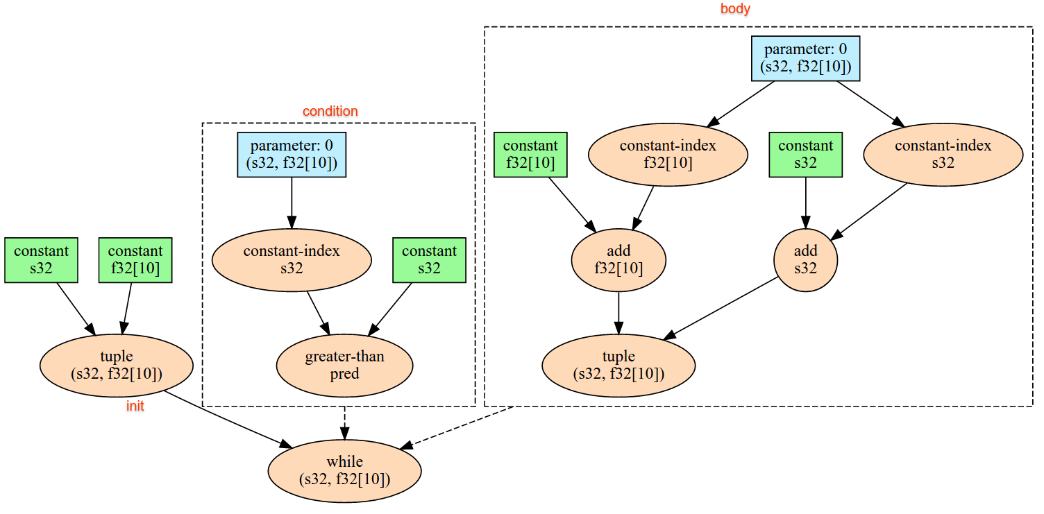
Đọc một mục dữ liệu từ giao diện truyền phát trong nguồn cấp dữ liệu ngầm ẩn của thiết bị, diễn giải dữ liệu dưới dạng hình dạng và bố cục đã cho, đồng thời trả về một XlaOp của dữ liệu. Cho phép nhiều thao tác trong nguồn cấp dữ liệu trong một tính toán, nhưng phải có tổng thứ tự trong số các thao tác trong nguồn cấp dữ liệu. Ví dụ: 2 Nguồn cấp dữ liệu trong mã bên dưới có tổng thứ tự vì có sự phụ thuộc giữa các vòng lặp while.
result1 = while (condition, init = init_value) {
  Infeed(shape)
}

result2 = while (condition, init = result1) {
  Infeed(shape)
}
Không hỗ trợ các hình dạng bộ dữ liệu lồng nhau. Đối với hình dạng bộ dữ liệu trống, thao tác Infeed sẽ không hoạt động và tiếp tục mà không cần đọc bất kỳ dữ liệu nào từ Infeed của thiết bị.
Iota
Hãy xem thêm XlaBuilder::Iota.
Iota(shape, iota_dimension)
Xây dựng một giá trị cố định liên tục trên thiết bị thay vì một hoạt động chuyển máy chủ lưu trữ lớn. Tạo một mảng có hình dạng đã chỉ định, đồng thời giữ các giá trị bắt đầu từ 0 và tăng dần từng giá trị một theo chiều được chỉ định. Đối với các loại dấu phẩy động, mảng được tạo tương đương với ConvertElementType(Iota(...)), trong đó Iota là loại tích phân và hoạt động chuyển đổi sẽ thành loại dấu phẩy động.
| Đối số | Loại | Ngữ nghĩa |
|---|---|---|
shape |
Shape |
Hình dạng của mảng do Iota() tạo |
iota_dimension |
int64 |
Phương diện sẽ tăng dần. |
Ví dụ: Iota(s32[4, 8], 0) trả về
  [[0, 0, 0, 0, 0, 0, 0, 0 ],
   [1, 1, 1, 1, 1, 1, 1, 1 ],
   [2, 2, 2, 2, 2, 2, 2, 2 ],
   [3, 3, 3, 3, 3, 3, 3, 3 ]]
Trả lại hàng với mức phí Iota(s32[4, 8], 1)
  [[0, 1, 2, 3, 4, 5, 6, 7 ],
   [0, 1, 2, 3, 4, 5, 6, 7 ],
   [0, 1, 2, 3, 4, 5, 6, 7 ],
   [0, 1, 2, 3, 4, 5, 6, 7 ]]
Bản đồ
Hãy xem thêm XlaBuilder::Map.
Map(operands..., computation)
| Đối số | Loại | Ngữ nghĩa |
|---|---|---|
operands |
chuỗi N XlaOp giây |
N mảng thuộc loại T0..T{N-1} |
computation |
XlaComputation |
tính toán kiểu T_0, T_1, .., T_{N + M -1} -> S với N tham số thuộc kiểu T và M thuộc kiểu tuỳ ý |
dimensions |
Mảng int64 |
mảng kích thước bản đồ |
Áp dụng hàm vô hướng trên các mảng operands đã cho, tạo ra một mảng có cùng kích thước, trong đó mỗi phần tử là kết quả của hàm được liên kết, áp dụng cho các phần tử tương ứng trong mảng đầu vào.
Hàm được ánh xạ là một phép tính tuỳ ý có giới hạn là hàm này có N đầu vào thuộc kiểu vô hướng T và một đầu ra duy nhất thuộc kiểu S. Kết quả đầu ra có cùng kích thước với toán hạng ngoại trừ việc loại phần tử T được thay thế bằng S.
Ví dụ: Map(op1, op2, op3, computation, par1) liên kết elem_out <-
computation(elem1, elem2, elem3, par1) tại mỗi chỉ mục (đa chiều) trong các mảng đầu vào để tạo ra mảng đầu ra.
OptimizationBarrier
Chặn mọi lượt tối ưu hoá khi di chuyển các phép tính qua rào cản.
Đảm bảo tất cả dữ liệu đầu vào đều được đánh giá trước bất kỳ toán tử nào phụ thuộc vào kết quả của rào cản.
Miếng đệm
Hãy xem thêm XlaBuilder::Pad.
Pad(operand, padding_value, padding_config)
| Đối số | Loại | Ngữ nghĩa |
|---|---|---|
operand |
XlaOp |
mảng thuộc loại T |
padding_value |
XlaOp |
đại lượng vô hướng thuộc kiểu T để lấp đầy khoảng đệm đã thêm |
padding_config |
PaddingConfig |
khoảng đệm ở cả hai cạnh (thấp, cao) và giữa các phần tử của mỗi chiều |
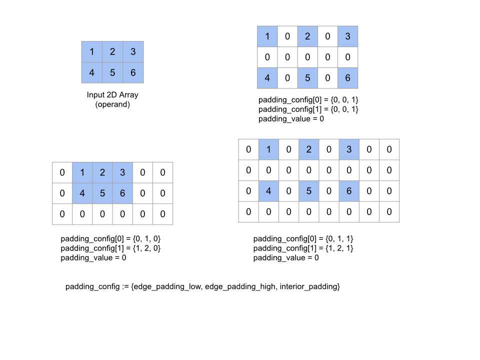
Mở rộng mảng operand đã cho bằng khoảng đệm xung quanh mảng cũng như giữa các phần tử của mảng có padding_value đã cho. padding_config chỉ định số lượng khoảng đệm cạnh và khoảng đệm bên trong cho mỗi kích thước.
PaddingConfig là một trường lặp lại của PaddingConfigDimension, chứa 3 trường cho mỗi chiều: edge_padding_low, edge_padding_high và interior_padding.
edge_padding_low và edge_padding_high chỉ định số lượng khoảng đệm đã thêm ở cấp thấp (bên cạnh chỉ mục 0) và cao cấp (bên cạnh chỉ mục cao nhất) của từng chiều tương ứng. Số lượng khoảng đệm cạnh có thể là số âm – giá trị tuyệt đối của khoảng đệm âm cho biết số phần tử cần xoá khỏi kích thước đã chỉ định.
interior_padding chỉ định khoảng đệm được thêm vào giữa hai phần tử bất kỳ trong mỗi chiều; khoảng đệm này không được là số âm. Khoảng đệm nội thất xảy ra theo logic trước khoảng đệm cạnh. Vì vậy, trong trường hợp khoảng đệm cạnh âm, các phần tử sẽ bị xoá khỏi toán hạng có khoảng đệm bên trong.
Thao tác này không hoạt động nếu các cặp khoảng đệm cạnh đều là (0, 0) và giá trị khoảng đệm bên trong đều là 0. Hình dưới đây cho thấy ví dụ về các giá trị edge_padding và interior_padding khác nhau cho một mảng hai chiều.
Recv
Hãy xem thêm XlaBuilder::Recv.
Recv(shape, channel_handle)
| Đối số | Loại | Ngữ nghĩa |
|---|---|---|
shape |
Shape |
hình dạng của dữ liệu cần nhận |
channel_handle |
ChannelHandle |
mã nhận dạng duy nhất cho mỗi cặp gửi/nhận |
Nhận dữ liệu có hình dạng đã cho từ lệnh Send trong một phép tính khác có cùng tên người dùng kênh. Trả về một XlaOp cho dữ liệu đã nhận.
API ứng dụng khách của hoạt động Recv thể hiện hoạt động giao tiếp đồng bộ.
Tuy nhiên, lệnh này được phân tách nội bộ thành 2 lệnh HLO (Recv và RecvDone) để bật tính năng chuyển dữ liệu không đồng bộ. Hãy xem thêm HloInstruction::CreateRecv và HloInstruction::CreateRecvDone.
Recv(const Shape& shape, int64 channel_id)
Phân bổ tài nguyên cần thiết để nhận dữ liệu từ lệnh Send có cùng channel_id. Trả về ngữ cảnh cho các tài nguyên được phân bổ mà lệnh RecvDone sau đây sẽ sử dụng để chờ hoàn tất quá trình chuyển dữ liệu. Ngữ cảnh này là một bộ dữ liệu của {receive buffer (shape), mã nhận dạng yêu cầu (U32)} và chỉ có thể sử dụng theo lệnh RecvDone.
RecvDone(HloInstruction context)
Với ngữ cảnh được tạo bằng lệnh Recv, hãy chờ quá trình chuyển dữ liệu hoàn tất và trả về dữ liệu đã nhận.
Giảm bớt
Hãy xem thêm XlaBuilder::Reduce.
Áp dụng hàm rút gọn cho một hoặc nhiều mảng song song.
Reduce(operands..., init_values..., computation, dimensions)
| Đối số | Loại | Ngữ nghĩa |
|---|---|---|
operands |
Chuỗi N XlaOp |
N mảng thuộc loại T_0, ..., T_{N-1}. |
init_values |
Chuỗi N XlaOp |
N đại lượng vô hướng thuộc kiểu T_0, ..., T_{N-1}. |
computation |
XlaComputation |
phép tính kiểu T_0, ..., T_{N-1}, T_0, ..., T_{N-1} -> Collate(T_0, ..., T_{N-1}). |
dimensions |
Mảng int64 |
mảng kích thước không theo thứ tự để giảm. |
Trong trường hợp:
- N bắt buộc phải lớn hơn hoặc bằng 1.
- Việc tính toán phải có kết hợp "gần đúng" (xem bên dưới).
- Tất cả mảng đầu vào phải có cùng phương diện.
- Tất cả các giá trị ban đầu phải tạo thành một mã nhận dạng trong
computation. - Nếu
N = 1,Collate(T)sẽ làT. - Nếu
N > 1,Collate(T_0, ..., T_{N-1})là một bộ dữ liệu của phần tửNthuộc loạiT.
Thao tác này giúp giảm một hoặc nhiều kích thước của từng mảng đầu vào thành các đại lượng vô hướng.
Thứ hạng của mỗi mảng được trả về là rank(operand) - len(dimensions). Kết quả
của op là Collate(Q_0, ..., Q_N), trong đó Q_i là một mảng thuộc loại T_i,
kích thước được mô tả ở bên dưới.
Các phần phụ trợ khác nhau được phép liên kết lại phép tính rút gọn. Điều này có thể dẫn đến sự khác biệt về số, vì một số hàm rút gọn như phép cộng không liên kết với số thực. Tuy nhiên, nếu phạm vi dữ liệu bị hạn chế, thì việc thêm dấu phẩy động gần như đủ để kết hợp cho hầu hết các trường hợp sử dụng thực tế.
Ví dụ
Khi giảm trên một phương diện trong một mảng 1D bằng các giá trị [10, 11,
12, 13], với hàm rút gọn f (đây là computation), thì giá trị này có thể được tính như
f(10, f(11, f(12, f(init_value, 13)))
nhưng cũng có nhiều khả năng khác, ví dụ:
f(init_value, f(f(10, f(init_value, 11)), f(f(init_value, 12), f(init_value, 13))))
Sau đây là ví dụ giả mã sơ bộ về cách triển khai rút gọn, sử dụng phép tính tổng làm phép tính rút gọn với giá trị ban đầu là 0.
result_shape <- remove all dims in dimensions from operand_shape

# Iterate over all elements in result_shape. The number of r's here is equal
# to the rank of the result
for r0 in range(result_shape[0]), r1 in range(result_shape[1]), ...:
  # Initialize this result element
  result[r0, r1...] <- 0

  # Iterate over all the reduction dimensions
  for d0 in range(dimensions[0]), d1 in range(dimensions[1]), ...:
    # Increment the result element with the value of the operand's element.
    # The index of the operand's element is constructed from all ri's and di's
    # in the right order (by construction ri's and di's together index over the
    # whole operand shape).
    result[r0, r1...] += operand[ri... di]
Dưới đây là ví dụ về cách giảm mảng 2D (ma trận). Hình dạng có thứ hạng 2, chiều 0 của kích thước 2 và chiều 1 của kích thước 3:
Kết quả của việc giảm phương diện 0 hoặc 1 bằng hàm "thêm":
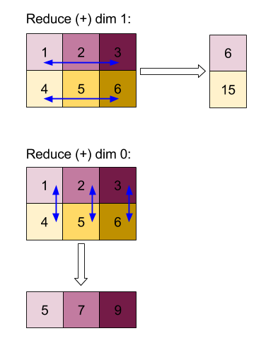
Lưu ý rằng cả hai kết quả rút gọn đều là mảng 1D. Sơ đồ cho thấy một mục ở dạng cột và một mục khác ở dạng hàng để thuận tiện cho hình ảnh.
Để tham khảo ví dụ phức tạp hơn, sau đây là mảng 3D. Thứ hạng của nó là 3, chiều 0 của kích thước 4, chiều 1 của kích thước 2 và chiều 2 của kích thước 3. Để đơn giản, các giá trị từ 1 đến 6 được sao chép trên chiều 0.
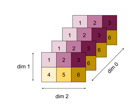
Tương tự như ví dụ 2D, chúng ta có thể chỉ giảm một kích thước. Ví dụ: nếu giảm phương diện 0, chúng ta sẽ nhận được một mảng hạng 2, trong đó tất cả các giá trị trên phương diện 0 được gộp lại thành một đại lượng vô hướng:
|  4   8  12 |
| 16  20  24 |
Nếu giảm chiều 2, chúng tôi cũng nhận được một mảng hạng-2, trong đó tất cả các giá trị trên phương diện 2 được thu gọn thành một đại lượng vô hướng:
| 6  15 |
| 6  15 |
| 6  15 |
| 6  15 |
Lưu ý rằng thứ tự tương đối giữa các kích thước còn lại trong dữ liệu đầu vào được giữ nguyên trong đầu ra, nhưng một số phương diện có thể được chỉ định số mới (do thứ hạng thay đổi).
Chúng ta cũng có thể giảm nhiều phương diện. Bổ sung kích thước 0 và 1 sẽ tạo ra mảng 1D [20, 28, 36].
Việc giảm mảng 3D trên tất cả các kích thước của mảng sẽ tạo ra đại lượng vô hướng 84.
Giảm đa dạng
Khi N > 1, việc áp dụng hàm giảm sẽ phức tạp hơn một chút vì hàm này được áp dụng đồng thời cho mọi dữ liệu đầu vào. Các toán hạng được cung cấp cho phép tính theo thứ tự sau:
- Chạy giá trị giảm cho toán hạng đầu tiên
- ...
- Chạy giá trị giảm cho toán hạng thứ N
- Giá trị đầu vào cho toán hạng đầu tiên
- ...
- Giá trị đầu vào cho toán hạng thứ N
Ví dụ: hãy xem xét hàm rút gọn sau đây (có thể dùng để tính song song giá trị tối đa và argmax của mảng 1-D):
f: (Float, Int, Float, Int) -> Float, Int
f(max, argmax, value, index):
  if value >= max:
    return (value, index)
  else:
    return (max, argmax)
Đối với các mảng Đầu vào 1-D V = Float[N], K = Int[N] và các giá trị khởi tạo I_V = Float, I_K = Int, kết quả f_(N-1) của việc giảm trên kích thước đầu vào duy nhất tương đương với ứng dụng đệ quy sau đây:
f_0 = f(I_V, I_K, V_0, K_0)
f_1 = f(f_0.first, f_0.second, V_1, K_1)
...
f_(N-1) = f(f_(N-2).first, f_(N-2).second, V_(N-1), K_(N-1))
Việc áp dụng rút gọn này cho một mảng giá trị và một mảng các chỉ số tuần tự (ví dụ: iota), sẽ lặp lại trên các mảng và trả về một bộ dữ liệu chứa giá trị tối đa và chỉ mục khớp.
ReducePrecision
Hãy xem thêm XlaBuilder::ReducePrecision.
Mô hình hoá tác động của việc chuyển đổi giá trị dấu phẩy động sang định dạng có độ chính xác thấp hơn (chẳng hạn như IEEE-FP16) và quay lại định dạng ban đầu. Bạn có thể tuỳ ý chỉ định số lượng bit số mũ và bit mantissa ở định dạng có độ chính xác thấp hơn, mặc dù tất cả kích thước bit có thể không được hỗ trợ trên mọi phương thức triển khai phần cứng.
ReducePrecision(operand, mantissa_bits, exponent_bits)
| Đối số | Loại | Ngữ nghĩa |
|---|---|---|
operand |
XlaOp |
kiểu dấu phẩy động T. |
exponent_bits |
int32 |
số bit số mũ ở định dạng độ chính xác thấp hơn |
mantissa_bits |
int32 |
số lượng bit mantissa ở định dạng có độ chính xác thấp hơn |
Kết quả thu được là một mảng thuộc loại T. Các giá trị đầu vào được làm tròn đến giá trị gần nhất biểu thị bằng số lượng bit mantissa đã cho (sử dụng ngữ nghĩa "liên kết với chẵn") và mọi giá trị vượt quá phạm vi được chỉ định theo số lượng bit số mũ đều được giới hạn thành vô cực dương hoặc âm. Các giá trị NaN sẽ được giữ lại, mặc dù các giá trị đó có thể được chuyển đổi thành giá trị NaN chính tắc.
Định dạng có độ chính xác thấp hơn phải có ít nhất một bit số mũ (để phân biệt giá trị 0 từ vô cực, vì cả hai đều có mantissa bằng 0) và phải có số bit mantissa không âm. Số lượng bit số mũ hoặc bit mantissa có thể vượt quá giá trị tương ứng cho loại T; phần tương ứng của lượt chuyển đổi khi đó sẽ chỉ đơn giản là không hoạt động.
ReduceScatter
Hãy xem thêm XlaBuilder::ReduceScatter.
Giảm Tán xạ là một hoạt động tập thể giúp thực hiện AllReduce một cách hiệu quả, sau đó phân tán kết quả bằng cách tách thành các khối shard_count dọc theo scatter_dimension và bản sao i trong nhóm bản sao sẽ nhận được phân đoạn ith.
ReduceScatter(operand, computation, scatter_dim, shard_count,
replica_group_ids, channel_id)
| Đối số | Loại | Ngữ nghĩa |
|---|---|---|
operand |
XlaOp |
Mảng hoặc một bộ dữ liệu không trống gồm các mảng để giảm bớt các bản sao. |
computation |
XlaComputation |
Tính toán rút gọn |
scatter_dimension |
int64 |
Phương diện cần phân tán. |
shard_count |
int64 |
Số khối cần tách: scatter_dimension |
replica_groups |
vectơ của các vectơ của int64 |
Các nhóm thực hiện việc cắt giảm |
channel_id |
int64 không bắt buộc |
Mã nhận dạng kênh không bắt buộc để giao tiếp giữa các mô-đun |
- Khi
operandlà một bộ dữ liệu của mảng, bộ tán xạ rút gọn sẽ được thực hiện trên từng phần tử của bộ dữ liệu. replica_groupslà một danh sách các nhóm bản sao được thực hiện trong quá trình rút gọn (có thể truy xuất mã bản sao của bản sao hiện tại bằng cách sử dụngReplicaId). Thứ tự của các bản sao trong mỗi nhóm sẽ xác định thứ tự phân tán kết quả giảm toàn bộ.replica_groupsphải để trống (trong trường hợp đó, mọi bản sao đều thuộc về một nhóm duy nhất) hoặc chứa cùng số phần tử với số lượng bản sao. Khi có nhiều nhóm bản sao, tất cả các nhóm đó phải có cùng kích thước. Ví dụ:replica_groups = {0, 2}, {1, 3}thực hiện giảm giữa các bản sao0và2, cũng như1và3, sau đó phân tán kết quả.shard_countlà kích thước của mỗi nhóm bản sao. Chúng ta cần điều này trong trường hợpreplica_groupstrống. Nếureplica_groupskhông trống,shard_countphải bằng kích thước của từng nhóm bản sao.channel_idđược dùng để giao tiếp trên nhiều mô-đun: chỉ các thao tácreduce-scattercó cùngchannel_idmới có thể giao tiếp với nhau.
Hình dạng đầu ra là hình dạng đầu vào với scatter_dimension được thu nhỏ hơn shard_count lần. Ví dụ: nếu có hai bản sao và toán tử có giá trị [1.0, 2.25] và [3.0, 5.25] tương ứng trên hai bản sao, thì giá trị đầu ra của thao tác này, trong đó scatter_dim là 0 sẽ là [4.0] cho bản sao đầu tiên và [7.5] cho bản sao thứ hai.
ReduceWindow
Hãy xem thêm XlaBuilder::ReduceWindow.
Áp dụng hàm rút gọn cho tất cả các phần tử trong mỗi cửa sổ của một chuỗi N mảng đa chiều, tạo ra một hoặc một bộ dữ liệu gồm N mảng đa chiều dưới dạng đầu ra. Mỗi mảng đầu ra có cùng số phần tử với số vị trí hợp lệ của cửa sổ. Lớp gộp có thể được biểu thị dưới dạng ReduceWindow. Tương tự như Reduce, computation được áp dụng luôn được chuyển init_values ở bên trái.
ReduceWindow(operands..., init_values..., computation, window_dimensions,
window_strides, padding)
| Đối số | Loại | Ngữ nghĩa |
|---|---|---|
operands |
N XlaOps |
Một chuỗi gồm N mảng đa chiều thuộc loại T_0,..., T_{N-1}, mỗi mảng đại diện cho vùng cơ sở nơi đặt cửa sổ. |
init_values |
N XlaOps |
Các giá trị bắt đầu của giá trị rút gọn, mỗi giá trị cho một toán hạng N. Xem phần Giảm thiểu để biết thông tin chi tiết. |
computation |
XlaComputation |
Hàm rút gọn thuộc kiểu T_0, ..., T_{N-1}, T_0, ..., T_{N-1} -> Collate(T_0, ..., T_{N-1}), để áp dụng cho các phần tử trong từng cửa sổ của tất cả các toán hạng đầu vào. |
window_dimensions |
ArraySlice<int64> |
mảng số nguyên cho các giá trị kích thước cửa sổ |
window_strides |
ArraySlice<int64> |
mảng số nguyên cho giá trị sải chân cửa sổ |
base_dilations |
ArraySlice<int64> |
mảng số nguyên cho các giá trị giãn cơ số |
window_dilations |
ArraySlice<int64> |
mảng số nguyên cho các giá trị mở rộng cửa sổ |
padding |
Padding |
loại khoảng đệm cho cửa sổ (Padding::kSame, đệm để có cùng hình dạng đầu ra như dữ liệu đầu vào nếu sải chân là 1, hoặc khoảng đệm::kValid, không sử dụng khoảng đệm và "dừng" cửa sổ khi không còn phù hợp) |
Trong trường hợp:
- N bắt buộc phải lớn hơn hoặc bằng 1.
- Tất cả mảng đầu vào phải có cùng phương diện.
- Nếu
N = 1,Collate(T)sẽ làT. - Nếu
N > 1,Collate(T_0, ..., T_{N-1})là một bộ dữ liệu của phần tửNthuộc loại(T0,...T{N-1}).
Mã và hình bên dưới là ví dụ về cách sử dụng ReduceWindow. Dữ liệu đầu vào là một ma trận có kích thước [4x6] và cả window_dimension và window_stride_dimension đều là [2x3].
// Create a computation for the reduction (maximum).
XlaComputation max;
{
  XlaBuilder builder(client_, "max");
  auto y = builder.Parameter(0, ShapeUtil::MakeShape(F32, {}), "y");
  auto x = builder.Parameter(1, ShapeUtil::MakeShape(F32, {}), "x");
  builder.Max(y, x);
  max = builder.Build().value();
}

// Create a ReduceWindow computation with the max reduction computation.
XlaBuilder builder(client_, "reduce_window_2x3");
auto shape = ShapeUtil::MakeShape(F32, {4, 6});
auto input = builder.Parameter(0, shape, "input");
builder.ReduceWindow(
    input,
    /*init_val=*/builder.ConstantLiteral(LiteralUtil::MinValue(F32)),
    *max,
    /*window_dimensions=*/{2, 3},
    /*window_stride_dimensions=*/{2, 3},
    Padding::kValid);
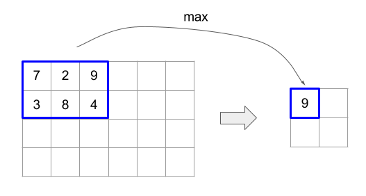
Bước 1 trong một phương diện cho biết vị trí của một cửa sổ trong phương diện cách cửa sổ liền kề 1 phần tử. Để chỉ định rằng không có cửa sổ nào trùng lặp với nhau, window_stride_dimension phải bằng window_dimension. Hình dưới đây minh hoạ cách sử dụng hai giá trị sải chân khác nhau. Khoảng đệm được áp dụng cho mỗi chiều của đầu vào và các phép tính giống như đầu vào với các kích thước sau khoảng đệm.
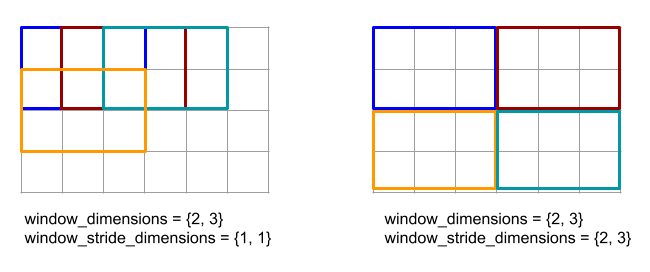
Đối với ví dụ về khoảng đệm không nhỏ, hãy cân nhắc tính toán giá trị tối thiểu của cửa sổ rút gọn (giá trị ban đầu là MAX_FLOAT) với kích thước 3 và sải chân 2 trên mảng đầu vào [10000, 1000, 100, 10, 1]. Khoảng đệm kValid tính toán mức tối thiểu trên hai cửa sổ hợp lệ: [10000, 1000, 100] và [100, 10, 1], dẫn đến đầu ra [100, 1]. Khoảng đệm kSame trước tiên sẽ dùng để đệm mảng để hình dạng sau cửa sổ thu nhỏ giống với dữ liệu đầu vào cho sải chân một bằng cách thêm các phần tử ban đầu ở cả hai bên, nhận được [MAX_VALUE, 10000, 1000, 100, 10, 1,
MAX_VALUE]. Việc chạy cửa sổ thu gọn trên mảng có đệm hoạt động trên 3 cửa sổ [MAX_VALUE, 10000, 1000], [1000, 100, 10], [10, 1, MAX_VALUE] và tạo ra [1000, 10, 1].
Thứ tự đánh giá của hàm rút gọn là tuỳ ý và có thể không xác định. Do đó, hàm rút gọn không nên quá nhạy cảm đối với việc liên kết lại. Hãy xem nội dung thảo luận về tính kết hợp trong ngữ cảnh Reduce để biết thêm thông tin chi tiết.
ReplicaId
Hãy xem thêm XlaBuilder::ReplicaId.
Trả về mã nhận dạng duy nhất (vô hướng U32) của bản sao.
ReplicaId()
Mã nhận dạng duy nhất của mỗi bản sao là một số nguyên chưa ký trong khoảng [0, N), trong đó N là số lượng bản sao. Vì tất cả bản sao đều đang chạy cùng một chương trình, nên lệnh gọi ReplicaId() trong chương trình sẽ trả về một giá trị riêng trên mỗi bản sao.
Đổi hình dạng
Hãy xem thêm XlaBuilder::Reshape và toán tử Collapse.
Định dạng lại kích thước của một mảng thành một cấu hình mới.
Reshape(operand, new_sizes)
Reshape(operand, dimensions, new_sizes)
| Đối số | Loại | Ngữ nghĩa |
|---|---|---|
operand |
XlaOp |
mảng loại T |
dimensions |
Vectơ int64 |
thứ tự thu gọn kích thước |
new_sizes |
Vectơ int64 |
vectơ có kích thước của các chiều mới |
Về mặt lý thuyết, trước tiên, hình dạng lại sẽ làm phẳng một mảng thành vectơ một chiều của các giá trị dữ liệu, sau đó tinh chỉnh vectơ này thành một hình dạng mới. Các đối số đầu vào là một mảng tuỳ ý thuộc loại T, vectơ hằng số tại thời gian biên dịch của các chỉ số chiều và một vectơ hằng số theo thời gian biên dịch của kích thước kích thước cho kết quả.
Các giá trị trong vectơ dimension, nếu có, phải là hoán vị của tất cả chiều của T; giá trị mặc định nếu không được cung cấp là {0, ..., rank - 1}. Thứ tự của các kích thước trong dimensions là từ chiều thay đổi chậm nhất (hầu hết chính) đến tham số thay đổi nhanh nhất (hầu hết nhỏ) trong nhóm vòng lặp. Hàm này sẽ thu gọn mảng đầu vào thành một chiều duy nhất. Vectơ new_sizes xác định kích thước của mảng đầu ra. Giá trị tại chỉ mục 0 trong new_sizes là kích thước của phương diện 0, giá trị ở chỉ mục 1 là kích thước của phương diện 1, v.v. Tích của các phương diện new_size phải bằng tích của các kích thước phương diện của toán hạng. Khi tinh chỉnh mảng đã thu gọn thành mảng đa chiều do new_sizes xác định, các kích thước trong new_sizes được sắp xếp theo thứ tự từ có mức thay đổi chậm nhất (lớn nhất) và đến nhanh nhất (hầu hết nhỏ).
Ví dụ: giả sử v là một mảng gồm 24 phần tử:
let v = f32[4x2x3] { { {10, 11, 12}, {15, 16, 17} },
                    { {20, 21, 22}, {25, 26, 27} },
                    { {30, 31, 32}, {35, 36, 37} },
                    { {40, 41, 42}, {45, 46, 47} } };

In-order collapse:
let v012_24 = Reshape(v, {0,1,2}, {24});
then v012_24 == f32[24] {10, 11, 12, 15, 16, 17, 20, 21, 22, 25, 26, 27,
                         30, 31, 32, 35, 36, 37, 40, 41, 42, 45, 46, 47};

let v012_83 = Reshape(v, {0,1,2}, {8,3});
then v012_83 == f32[8x3] { {10, 11, 12}, {15, 16, 17},
                          {20, 21, 22}, {25, 26, 27},
                          {30, 31, 32}, {35, 36, 37},
                          {40, 41, 42}, {45, 46, 47} };

Out-of-order collapse:
let v021_24 = Reshape(v, {1,2,0}, {24});
then v012_24 == f32[24]  {10, 20, 30, 40, 11, 21, 31, 41, 12, 22, 32, 42,
                          15, 25, 35, 45, 16, 26, 36, 46, 17, 27, 37, 47};

let v021_83 = Reshape(v, {1,2,0}, {8,3});
then v021_83 == f32[8x3] { {10, 20, 30}, {40, 11, 21},
                          {31, 41, 12}, {22, 32, 42},
                          {15, 25, 35}, {45, 16, 26},
                          {36, 46, 17}, {27, 37, 47} };


let v021_262 = Reshape(v, {1,2,0}, {2,6,2});
then v021_262 == f32[2x6x2] { { {10, 20}, {30, 40},
                              {11, 21}, {31, 41},
                              {12, 22}, {32, 42} },
                             { {15, 25}, {35, 45},
                              {16, 26}, {36, 46},
                              {17, 27}, {37, 47} } };
Trong một trường hợp đặc biệt, việc đổi hình dạng có thể biến đổi mảng một phần tử thành đại lượng vô hướng và ngược lại. Ví dụ:
Reshape(f32[1x1] { {5} }, {0,1}, {}) == 5;
Reshape(5, {}, {1,1}) == f32[1x1] { {5} };
Doanh thu (đảo ngược)
Hãy xem thêm XlaBuilder::Rev.
Rev(operand, dimensions)
| Đối số | Loại | Ngữ nghĩa |
|---|---|---|
operand |
XlaOp |
mảng loại T |
dimensions |
ArraySlice<int64> |
phương diện để đảo ngược |
Đảo ngược thứ tự của các phần tử trong mảng operand dọc theo dimensions được chỉ định, tạo ra một mảng đầu ra có cùng hình dạng. Mỗi phần tử của mảng toán hạng ở một chỉ mục đa chiều được lưu trữ vào mảng đầu ra ở một chỉ mục biến đổi. Chỉ mục đa chiều được biến đổi bằng cách đảo ngược chỉ mục trong từng chiều cần đảo ngược (nghĩa là nếu chiều có kích thước N là một trong các chiều đảo ngược, chỉ mục i của nó được chuyển đổi thành N – 1 – i).
Một cách sử dụng cho toán tử Rev là đảo ngược mảng trọng số tích chập dọc theo hai kích thước cửa sổ trong quá trình tính toán chuyển màu trong mạng nơron.
RngNormal
Hãy xem thêm XlaBuilder::RngNormal.
Tạo kết quả của một hình dạng cho trước bằng các số ngẫu nhiên được tạo theo \(N(\mu, \sigma)\) phân phối chuẩn. Các tham số \(\mu\) và \(\sigma\)và hình dạng đầu ra phải có kiểu phần tử dấu phẩy động. Các tham số hơn nữa phải có giá trị vô hướng.
RngNormal(mu, sigma, shape)
| Đối số | Loại | Ngữ nghĩa |
|---|---|---|
mu |
XlaOp |
Vô hướng thuộc loại T chỉ định giá trị trung bình của các số được tạo |
sigma |
XlaOp |
Giá trị vô hướng thuộc loại T chỉ định độ lệch chuẩn của giá trị đã tạo |
shape |
Shape |
Hình dạng đầu ra thuộc loại T |
RngUniform
Hãy xem thêm XlaBuilder::RngUniform.
Xây dựng đầu ra của một hình dạng cho trước với các số ngẫu nhiên được tạo sau sự phân phối đồng nhất trong khoảng \([a,b)\). Các tham số và loại phần tử đầu ra phải là loại boolean, loại tích phân hoặc loại dấu phẩy động và các loại phải nhất quán. Các phần phụ trợ CPU và GPU hiện chỉ hỗ trợ F64, F32, F16, BF16, S64, U64, S32 và U32. Hơn nữa, các tham số cần phải có giá trị vô hướng. Nếu \(b <= a\) kết quả được xác định theo mô hình triển khai.
RngUniform(a, b, shape)
| Đối số | Loại | Ngữ nghĩa |
|---|---|---|
a |
XlaOp |
Giá trị vô hướng của loại T xác định giới hạn dưới của khoảng |
b |
XlaOp |
Giá trị vô hướng thuộc loại T xác định giới hạn trên của khoảng |
shape |
Shape |
Hình dạng đầu ra thuộc loại T |
RngBitGenerator
Tạo đầu ra có hình dạng nhất định chứa các bit ngẫu nhiên đồng nhất bằng cách sử dụng thuật toán đã chỉ định (hoặc giá trị mặc định phụ trợ) và trả về trạng thái cập nhật (có hình dạng giống như trạng thái ban đầu) và dữ liệu ngẫu nhiên được tạo.
Trạng thái ban đầu là trạng thái ban đầu của quá trình tạo số ngẫu nhiên hiện tại. Hình dạng này cũng như hình dạng bắt buộc và các giá trị hợp lệ phụ thuộc vào thuật toán được sử dụng.
Kết quả đầu ra được đảm bảo là hàm tất định của trạng thái ban đầu, nhưng không đảm bảo có tính xác định giữa các phần phụ trợ và các phiên bản trình biên dịch khác nhau.
RngBitGenerator(algorithm, key, shape)
| Đối số | Loại | Ngữ nghĩa |
|---|---|---|
algorithm |
RandomAlgorithm |
Thuật toán PRNG sẽ được sử dụng. |
initial_state |
XlaOp |
Trạng thái ban đầu của thuật toán PRNG. |
shape |
Shape |
Hình dạng đầu ra cho dữ liệu đã tạo. |
Các giá trị có thể sử dụng cho trường algorithm:
rng_default: Thuật toán dành riêng cho phần phụ trợ với các yêu cầu về hình dạng cụ thể cho phần phụ trợ.rng_three_fry: Thuật toán PRNG dựa trên bộ đếm ThreeFry. Hình dạnginitial_statelàu64[2]với các giá trị tuỳ ý. Salmon và cộng sự SC 2011. Số ngẫu nhiên song song: dễ như 1, 2, 3.rng_philox: Thuật toán Philox để tạo song song các số ngẫu nhiên. Hình dạnginitial_statelàu64[3]với các giá trị tuỳ ý. Salmon và cộng sự SC 2011. Số ngẫu nhiên song song: dễ như 1, 2, 3.
Tán xạ
Thao tác tán xạ XLA tạo ra một chuỗi kết quả là các giá trị của mảng đầu vào operands, trong đó một số lát cắt (tại các chỉ mục do scatter_indices chỉ định) được cập nhật bằng trình tự các giá trị trong updates bằng update_computation.
Hãy xem thêm XlaBuilder::Scatter.
scatter(operands..., scatter_indices, updates..., update_computation,
index_vector_dim, update_window_dims, inserted_window_dims,
scatter_dims_to_operand_dims)
| Đối số | Loại | Ngữ nghĩa |
|---|---|---|
operands |
Chuỗi N XlaOp |
N mảng thuộc loại T_0, ..., T_N được phân tán. |
scatter_indices |
XlaOp |
Mảng chứa chỉ mục bắt đầu của các lát cắt phải được phân tán. |
updates |
Chuỗi N XlaOp |
N mảng thuộc loại T_0, ..., T_N. updates[i] chứa các giá trị phải được dùng để tán xạ operands[i]. |
update_computation |
XlaComputation |
Phép tính được dùng để kết hợp các giá trị hiện có trong mảng đầu vào và các nội dung cập nhật trong quá trình phân tán. Phép tính này phải thuộc kiểu T_0, ..., T_N, T_0, ..., T_N -> Collate(T_0, ..., T_N). |
index_vector_dim |
int64 |
Phương diện trong scatter_indices chứa các chỉ mục bắt đầu. |
update_window_dims |
ArraySlice<int64> |
Tập hợp kích thước trong hình dạng updates là kích thước cửa sổ. |
inserted_window_dims |
ArraySlice<int64> |
Tập hợp kích thước cửa sổ phải được chèn vào hình dạng updates. |
scatter_dims_to_operand_dims |
ArraySlice<int64> |
Phương diện ánh xạ từ chỉ mục tán xạ đến không gian chỉ mục toán hạng. Mảng này được thể hiện dưới dạng ánh xạ i đến scatter_dims_to_operand_dims[i] . Chương trình phải diễn ra 1:1 và toàn bộ. |
indices_are_sorted |
bool |
Liệu các chỉ mục có được đảm bảo sắp xếp theo phương thức gọi hay không. |
Trong trường hợp:
- N bắt buộc phải lớn hơn hoặc bằng 1.
operands[0], ...,operands[N-1] phải có cùng phương diện.updates[0], ...,updates[N-1] phải có cùng phương diện.- Nếu
N = 1,Collate(T)sẽ làT. - Nếu
N > 1,Collate(T_0, ..., T_N)là một bộ dữ liệu của phần tửNthuộc loạiT.
Nếu index_vector_dim bằng scatter_indices.rank, chúng tôi ngầm coi scatter_indices có phương diện 1 cuối.
Chúng ta xác định update_scatter_dims thuộc loại ArraySlice<int64> là tập hợp kích thước thuộc hình dạng updates. Không phải trong update_window_dims, theo thứ tự tăng dần.
Các đối số của tán xạ phải tuân theo các quy tắc ràng buộc sau:
Mỗi mảng
updatesphải có thứ hạngupdate_window_dims.size + scatter_indices.rank - 1.Giới hạn của kích thước
itrong mỗi mảngupdatesphải tuân theo các giới hạn sau:- Nếu
icó trongupdate_window_dims(tức là bằngupdate_window_dims[k] đối với một sốk), thì giới hạn của kích thướcitrongupdateskhông được vượt quá giới hạn tương ứng củaoperandsau khi tính đếninserted_window_dims(tức làadjusted_window_bounds[k], trong đóadjusted_window_boundschứa giới hạn củaoperandvới giới hạn tại các chỉ mục đã bị xoáinserted_window_dims). - Nếu
icó trongupdate_scatter_dims(tức là bằngupdate_scatter_dims[k] đối với một sốk), thì giới hạn của phương diệnitrongupdatesphải bằng với giới hạn tương ứng củascatter_indices, bỏ quaindex_vector_dim(tức làscatter_indices.shape.dims[k], nếuk<index_vector_dimvà ngược lại làscatter_indices.shape.dims[k+1]).
- Nếu
update_window_dimsphải theo thứ tự tăng dần, không có số phương diện lặp lại và nằm trong phạm vi[0, updates.rank).inserted_window_dimsphải theo thứ tự tăng dần, không có số phương diện lặp lại và nằm trong phạm vi[0, operand.rank).operand.rankphải bằng tổng củaupdate_window_dims.sizevàinserted_window_dims.size.scatter_dims_to_operand_dims.sizephải bằngscatter_indices.shape.dims[index_vector_dim] và giá trị của thuộc tính này phải nằm trong phạm vi[0, operand.rank).
Đối với một chỉ mục U nhất định trong mỗi mảng updates, chỉ mục I tương ứng trong mảng operands tương ứng mà bản cập nhật này phải được áp dụng sẽ được tính như sau:
- Đặt
G= {U[k] choktrongupdate_scatter_dims}. DùngGđể tra cứu vectơ chỉ mụcStrong mảngscatter_indicessao choS[i] =scatter_indices[Kết hợp(G,i)] trong đó Kết hợp(A, b) chèn b tại vị tríindex_vector_dimvào A. - Tạo một chỉ mục
Sinvàooperandbằng cách sử dụngSbằng cách phân tánSbằng bản đồscatter_dims_to_operand_dims. Chính thức hơn:Sin[scatter_dims_to_operand_dims[k]] =S[k] nếuk<scatter_dims_to_operand_dims.size.Sin[_] =0nếu không.
- Tạo chỉ mục
Winvào từng mảngoperandsbằng cách phân tán các chỉ mục tạiupdate_window_dimstrongUtheoinserted_window_dims. Chính thức hơn:Win[window_dims_to_operand_dims(k)] =U[k] nếuknằm trongupdate_window_dims, trong đówindow_dims_to_operand_dimslà hàm đơn điệu có miền [0,update_window_dims.size) và dải ô [0,operand.rank) \inserted_window_dims. (Ví dụ: nếuupdate_window_dims.sizelà4,operand.ranklà6vàinserted_window_dimslà {0,2}, thìwindow_dims_to_operand_dimslà {0→1,1→3,2→4,3→5}).Win[_] =0nếu không.
IlàWin+Sin, trong đó + là phép cộng theo phần tử.
Tóm lại, thao tác tán xạ có thể được định nghĩa như sau.
- Khởi động
outputvớioperands, tức là cho tất cả các chỉ mụcJ, cho tất cả chỉ mụcOtrong mảngoperands[J]:
output[J][O] =operands[J][O] - Đối với mọi chỉ mục
Utrong mảngupdates[J] và chỉ mục tương ứngOtrong mảngoperand[J], nếuOlà chỉ mục hợp lệ chooutput:
(output[0][O], ...,output[N-1][O]) =update_computation(output[0][O], ..., ,output[N-1][O],updates[0][U], ...,updates[N-1][U])
Thứ tự áp dụng các bản cập nhật là không xác định. Do đó, khi nhiều chỉ mục trong updates tham chiếu đến cùng một chỉ mục trong operands, giá trị tương ứng trong output sẽ không xác định.
Xin lưu ý rằng tham số đầu tiên được truyền vào update_computation sẽ luôn là giá trị hiện tại từ mảng output và tham số thứ hai sẽ luôn là giá trị từ mảng updates. Điều này rất quan trọng đối với các trường hợp khi update_computation không có tính chất giao hoán.
Nếu bạn đặt indices_are_sorted thành true (đúng), thì XLA có thể giả định rằng start_indices được người dùng sắp xếp (theo thứ tự start_index_map tăng dần). Nếu không thì ngữ nghĩa sẽ được xác định.
Một cách không chính thức, bạn có thể xem hoạt động phân tán ngược của hoạt động thu thập, tức là hoạt động phân tán sẽ cập nhật các phần tử trong dữ liệu đầu vào được trích xuất bằng hoạt động thu thập tương ứng.
Để xem các ví dụ và nội dung mô tả không chính thức chi tiết, hãy tham khảo mục "Mô tả không chính thức" trong Gather.
Chọn
Hãy xem thêm XlaBuilder::Select.
Tạo một mảng đầu ra từ các phần tử của 2 mảng đầu vào, dựa trên các giá trị của một mảng vị từ.
Select(pred, on_true, on_false)
| Đối số | Loại | Ngữ nghĩa |
|---|---|---|
pred |
XlaOp |
mảng thuộc loại PRED |
on_true |
XlaOp |
mảng loại T |
on_false |
XlaOp |
mảng loại T |
Các mảng on_true và on_false phải có cùng hình dạng. Đây cũng là hình dạng của mảng đầu ra. Mảng pred phải có cùng số chiều với on_true và on_false với loại phần tử PRED.
Đối với mỗi phần tử P của pred, phần tử tương ứng của mảng đầu ra sẽ được lấy từ on_true nếu giá trị của P là true và từ on_false nếu giá trị của P là false. Ở một dạng thông báo truyền tin bị hạn chế, pred có thể là đại lượng vô hướng thuộc kiểu PRED. Trong trường hợp này, mảng đầu ra được lấy hoàn toàn từ on_true nếu pred là true và từ on_false nếu pred là false.
Ví dụ với pred không vô hướng:
let pred: PRED[4] = {true, false, false, true};
let v1: s32[4] = {1, 2, 3, 4};
let v2: s32[4] = {100, 200, 300, 400};
==>
Select(pred, v1, v2) = s32[4]{1, 200, 300, 4};
Ví dụ với pred vô hướng:
let pred: PRED = true;
let v1: s32[4] = {1, 2, 3, 4};
let v2: s32[4] = {100, 200, 300, 400};
==>
Select(pred, v1, v2) = s32[4]{1, 2, 3, 4};
Hỗ trợ lựa chọn giữa các bộ dữ liệu. Tuples được coi là kiểu vô hướng cho mục đích này. Nếu on_true và on_false là bộ dữ liệu (phải có cùng hình dạng!) thì pred phải là đại lượng vô hướng có kiểu PRED.
SelectAndScatter
Hãy xem thêm XlaBuilder::SelectAndScatter.
Toán tử này có thể được xem là toán tử kết hợp, trước tiên sẽ tính toán ReduceWindow trên mảng operand để chọn một phần tử từ mỗi cửa sổ, sau đó phân tán mảng source đến chỉ mục của các phần tử đã chọn để tạo một mảng đầu ra có hình dạng giống với mảng toán hạng. Hàm select nhị phân được dùng để chọn một phần tử từ mỗi cửa sổ bằng cách áp dụng hàm đó trên từng cửa sổ và hàm này được gọi bằng thuộc tính mà vectơ chỉ mục của tham số đầu tiên nhỏ hơn vectơ chỉ mục của tham số thứ hai về mặt từ vựng. Hàm select trả về true nếu tham số đầu tiên được chọn và trả về false nếu tham số thứ hai được chọn, đồng thời hàm phải duy trì tính bắc cầu (tức là nếu select(a, b) và select(b, c) là true, thì select(a, c) cũng là true) để phần tử được chọn không phụ thuộc vào thứ tự của các phần tử được truyền tải trong một cửa sổ nhất định.
Hàm scatter được áp dụng tại mỗi chỉ mục đã chọn trong mảng đầu ra. Phương thức này sử dụng 2 tham số vô hướng:
- Giá trị hiện tại tại chỉ mục đã chọn trong mảng đầu ra
- Giá trị tán xạ từ
sourceáp dụng cho chỉ mục đã chọn
Phương thức này kết hợp 2 tham số rồi trả về một giá trị vô hướng dùng để cập nhật giá trị tại chỉ mục đã chọn trong mảng đầu ra. Ban đầu, tất cả các chỉ mục của mảng đầu ra được đặt thành init_value.
Mảng đầu ra có cùng hình dạng với mảng operand và mảng source phải có cùng hình dạng như kết quả của việc áp dụng toán tử ReduceWindow trên mảng operand. Bạn có thể sử dụng SelectAndScatter để truyền ngược các giá trị độ dốc cho một lớp gộp trong mạng nơron.
SelectAndScatter(operand, select, window_dimensions, window_strides,
padding, source, init_value, scatter)
| Đối số | Loại | Ngữ nghĩa |
|---|---|---|
operand |
XlaOp |
mảng loại T mà cửa sổ trượt qua |
select |
XlaComputation |
Phép tính nhị phân thuộc kiểu T, T -> PRED, để áp dụng cho tất cả phần tử trong từng cửa sổ; trả về true nếu tham số đầu tiên được chọn và trả về false nếu tham số thứ hai được chọn |
window_dimensions |
ArraySlice<int64> |
mảng số nguyên cho các giá trị kích thước cửa sổ |
window_strides |
ArraySlice<int64> |
mảng số nguyên cho giá trị sải chân cửa sổ |
padding |
Padding |
Loại khoảng đệm cho cửa sổ (Khoảng đệm::kSame hoặc Khoảng đệm::kValid) |
source |
XlaOp |
mảng loại T với các giá trị cần phân tán |
init_value |
XlaOp |
giá trị vô hướng của loại T cho giá trị ban đầu của mảng đầu ra |
scatter |
XlaComputation |
phép tính nhị phân thuộc kiểu T, T -> T, để áp dụng từng phần tử nguồn phân tán cùng với phần tử đích |
Hình dưới đây là các ví dụ về cách sử dụng SelectAndScatter, trong đó select
tính giá trị tối đa trong số các tham số của hàm đó. Lưu ý rằng khi các cửa sổ chồng chéo nhau, như trong hình (2) bên dưới, một chỉ mục của mảng operand có thể được chọn nhiều lần theo các cửa sổ khác nhau. Trong hình, phần tử của giá trị 9 được cả hai cửa sổ trên cùng (xanh dương và đỏ) chọn và hàm cộng nhị phân scatter sẽ tạo ra phần tử đầu ra có giá trị 8 (2 + 6).
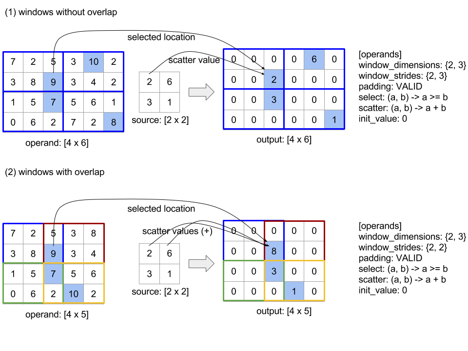
Thứ tự đánh giá của hàm scatter là tuỳ ý và có thể không xác định. Do đó, hàm scatter không nên quá nhạy cảm đối với việc liên kết lại. Hãy xem nội dung thảo luận về tính kết hợp trong ngữ cảnh Reduce để biết thêm thông tin chi tiết.
Gửi
Hãy xem thêm XlaBuilder::Send.
Send(operand, channel_handle)
| Đối số | Loại | Ngữ nghĩa |
|---|---|---|
operand |
XlaOp |
dữ liệu cần gửi (mảng loại T) |
channel_handle |
ChannelHandle |
mã nhận dạng duy nhất cho mỗi cặp gửi/nhận |
Gửi dữ liệu toán hạng đã cho đến một lệnh Recv trong một phép tính khác có cùng tên người dùng kênh. Không trả về bất kỳ dữ liệu nào.
Tương tự như thao tác Recv, API ứng dụng của thao tác Send đại diện cho hoạt động giao tiếp đồng bộ và được phân tách nội bộ thành 2 lệnh HLO (Send và SendDone) để cho phép chuyển dữ liệu không đồng bộ. Hãy xem thêm HloInstruction::CreateSend và HloInstruction::CreateSendDone.
Send(HloInstruction operand, int64 channel_id)
Bắt đầu chuyển không đồng bộ toán hạng sang tài nguyên do lệnh Recv phân bổ có cùng mã nhận dạng kênh. Trả về ngữ cảnh mà lệnh SendDone sau đây sử dụng để chờ hoàn tất quá trình chuyển dữ liệu. Ngữ cảnh này là một bộ dữ liệu của {operand (shape), giá trị nhận dạng yêu cầu (U32)} và chỉ có thể sử dụng theo lệnh SendDone.
SendDone(HloInstruction context)
Với ngữ cảnh do lệnh Send tạo, hãy đợi quá trình chuyển dữ liệu hoàn tất. Lệnh này không trả về bất kỳ dữ liệu nào.
Lên lịch hướng dẫn kênh
Thứ tự thực thi 4 lệnh cho mỗi kênh (Recv, RecvDone,
Send, SendDone) như sau.
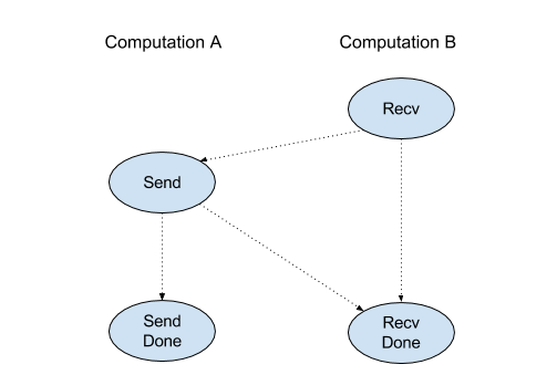
Recvdiễn ra trướcSendSenddiễn ra trướcRecvDoneRecvdiễn ra trướcRecvDoneSenddiễn ra trướcSendDone
Khi các trình biên dịch phụ trợ tạo lịch biểu tuyến tính cho mỗi phép tính giao tiếp thông qua hướng dẫn kênh, không được có chu kỳ giữa các phép tính. Ví dụ: các lịch biểu bên dưới dẫn đến tắc nghẽn.
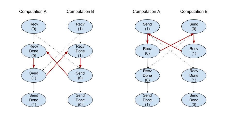
Slice (lát cắt)
Hãy xem thêm XlaBuilder::Slice.
Cắt lát sẽ trích xuất một mảng con trong mảng đầu vào. Mảng con có cùng thứ hạng với đầu vào và chứa các giá trị bên trong hộp giới hạn bên trong mảng đầu vào, nơi mà các kích thước và chỉ mục của hộp giới hạn được cung cấp làm đối số cho thao tác lát cắt.
Slice(operand, start_indices, limit_indices, strides)
| Đối số | Loại | Ngữ nghĩa |
|---|---|---|
operand |
XlaOp |
Mảng thứ nguyên loại T |
start_indices |
ArraySlice<int64> |
Danh sách N số nguyên có chứa các chỉ mục bắt đầu của lát cắt cho mỗi chiều. Giá trị phải lớn hơn hoặc bằng 0. |
limit_indices |
ArraySlice<int64> |
Danh sách N số nguyên có chứa các chỉ mục kết thúc (ngoại trừ) cho lát cắt của từng phương diện. Mỗi giá trị phải lớn hơn hoặc bằng giá trị start_indices tương ứng của phương diện này và nhỏ hơn hoặc bằng kích thước của phương diện này. |
strides |
ArraySlice<int64> |
Danh sách số nguyên N quyết định bước tiến đầu vào của lát cắt. Lát cắt chọn mọi phần tử strides[d] trong phương diện d. |
Ví dụ về 1 phương diện:
let a = {0.0, 1.0, 2.0, 3.0, 4.0}
Slice(a, {2}, {4}) produces:
  {2.0, 3.0}
Ví dụ về 2 chiều:
let b =
 { {0.0,  1.0,  2.0},
   {3.0,  4.0,  5.0},
   {6.0,  7.0,  8.0},
   {9.0, 10.0, 11.0} }

Slice(b, {2, 1}, {4, 3}) produces:
  { { 7.0,  8.0},
    {10.0, 11.0} }
Sắp xếp
Hãy xem thêm XlaBuilder::Sort.
Sort(operands, comparator, dimension, is_stable)
| Đối số | Loại | Ngữ nghĩa |
|---|---|---|
operands |
ArraySlice<XlaOp> |
Các toán hạng cần sắp xếp. |
comparator |
XlaComputation |
Phép tính so sánh sẽ sử dụng. |
dimension |
int64 |
Phương diện cần sắp xếp. |
is_stable |
bool |
Có nên sử dụng cách sắp xếp ổn định hay không. |
Nếu chỉ cung cấp một toán hạng:
Nếu toán hạng là một tensor xếp hạng-1 (một mảng), kết quả là một mảng được sắp xếp. Nếu bạn muốn sắp xếp mảng theo thứ tự tăng dần, trình so sánh sẽ thực hiện phép so sánh nhỏ hơn. Chính thức, sau khi được sắp xếp, mảng sẽ áp dụng cho mọi vị trí chỉ mục
i, jvớii < jlàcomparator(value[i], value[j]) = comparator(value[j], value[i]) = falsehoặccomparator(value[i], value[j]) = true.Nếu toán hạng có thứ hạng cao hơn, thì toán hạng sẽ được sắp xếp theo phương diện đã cho. Ví dụ: đối với tensor hạng 2 (ma trận), giá trị chiều của
0sẽ sắp xếp độc lập từng cột và giá trị chiều là1sẽ sắp xếp độc lập từng hàng. Nếu bạn không cung cấp số phương diện, thì phương diện gần đây nhất sẽ được chọn theo mặc định. Đối với thứ nguyên được sắp xếp, thứ tự sắp xếp áp dụng tương tự như trong trường hợp xếp hạng-1.
Nếu bạn cung cấp toán hạng n > 1:
Tất cả toán hạng
nphải là tensor có cùng chiều. Các loại phần tử của tensor có thể khác nhau.Tất cả các toán hạng được sắp xếp cùng nhau, không phải riêng lẻ. Về mặt lý thuyết, toán hạng được coi là một bộ dữ liệu. Khi kiểm tra xem các phần tử của mỗi toán hạng tại các vị trí chỉ mục
ivàjcó cần được hoán đổi hay không, trình so sánh sẽ được gọi bằng tham số vô hướng2 * n, trong đó tham số2 * ktương ứng với giá trị ở vị tríitừ toán hạngk-thvà tham số2 * k + 1tương ứng với giá trị ở vị tríjtừ toán hạngk-th. Do đó, trình so sánh sẽ so sánh các tham số2 * kvà2 * k + 1với nhau, cũng như có thể sử dụng các cặp tham số khác làm yếu tố ràng buộc.Kết quả là một bộ dữ liệu bao gồm các toán hạng theo thứ tự được sắp xếp (theo chiều được cung cấp như ở trên). Toán hạng
i-thcủa bộ dữ liệu tương ứng với toán hạngi-thcủa Sắp xếp.
Ví dụ: nếu có ba toán hạng operand0 = [3, 1], operand1 = [42, 50], operand2 = [-3.0, 1.1] và trình so sánh chỉ so sánh các giá trị của operand0 với nhỏ hơn, thì kết quả của loại này là bộ dữ liệu ([1, 3], [50, 42], [1.1, -3.0]).
Nếu bạn đặt is_stable thành true, thì hệ thống sẽ đảm bảo hệ thống sắp xếp ổn định, nghĩa là nếu có các phần tử được trình so sánh coi là bằng nhau, thì thứ tự tương đối của các giá trị bằng nhau sẽ được giữ nguyên. Hai phần tử e1 và e2 là bằng nhau khi và chỉ khi comparator(e1, e2) = comparator(e2, e1) = false. Theo mặc định, is_stable được đặt thành false.
Hoán vị
Hãy xem thêm toán tử tf.reshape.
Transpose(operand)
| Đối số | Loại | Ngữ nghĩa |
|---|---|---|
operand |
XlaOp |
Toán hạng để hoán vị. |
permutation |
ArraySlice<int64> |
Cách hiển thị các phương diện. |
Hoán vị các chiều của toán hạng với phép hoán vị đã cho, vì vậy, ∀ i . 0 ≤ i < rank ⇒ input_dimensions[permutation[i]] = output_dimensions[i].
Điều này giống như Reshape(toán hạng, hoán vị, Permute(hoá vị, toán hạng.shape.dimension)).
TriangularSolve
Hãy xem thêm XlaBuilder::TriangularSolve.
Giải các hệ phương trình tuyến tính có ma trận hệ số tam giác trên hoặc dưới bằng phép thế tiến hoặc thế lùi. Việc phát theo các chiều chính, quy trình này sẽ giải quyết một trong các hệ thống ma trận op(a) * x =
b hoặc x * op(a) = b cho biến x, cho a và b, trong đó op(a) là op(a) = a, op(a) = Transpose(a) hoặc op(a) = Conj(Transpose(a)).
TriangularSolve(a, b, left_side, lower, unit_diagonal, transpose_a)
| Đối số | Loại | Ngữ nghĩa |
|---|---|---|
a |
XlaOp |
một mảng > 2 thuộc một kiểu phức tạp hoặc dấu phẩy động có hình dạng [..., M, M]. |
b |
XlaOp |
một mảng > 2 cùng loại có hình dạng [..., M, K] nếu left_side là đúng, nếu không thì [..., K, M]. |
left_side |
bool |
cho biết sẽ giải hệ dưới dạng op(a) * x = b (true) hay x * op(a) = b (false). |
lower |
bool |
liệu sử dụng tam giác trên hay tam giác dưới của a. |
unit_diagonal |
bool |
nếu là true, các phần tử đường chéo của a được giả định là 1 và không được truy cập. |
transpose_a |
Transpose |
cho dù là sử dụng a nguyên trạng, hoán vị hay thực hiện hoán vị liên hợp. |
Dữ liệu đầu vào chỉ được đọc từ tam giác dưới/trên của a, tuỳ thuộc vào giá trị của lower. Các giá trị từ tam giác khác sẽ bị bỏ qua. Dữ liệu đầu ra được trả về trong cùng một tam giác; các giá trị trong tam giác khác được xác định theo phương thức triển khai và có thể là bất kỳ giá trị nào.
Nếu thứ hạng của a và b lớn hơn 2, thì các giá trị này được coi là nhóm ma trận, trong đó tất cả ngoại trừ 2 kích thước nhỏ đều là kích thước lô. a và b phải có kích thước lô bằng nhau.
Bộ xếp
Hãy xem thêm XlaBuilder::Tuple.
Một bộ dữ liệu chứa nhiều đối tượng xử lý dữ liệu, mỗi đối tượng có hình dạng riêng.
Hàm này tương tự như std::tuple trong C++. Về mặt lý thuyết:
let v: f32[10] = f32[10]{0, 1, 2, 3, 4, 5, 6, 7, 8, 9};
let s: s32 = 5;
let t: (f32[10], s32) = tuple(v, s);
Bạn có thể giải cấu trúc (truy cập) cặp dữ liệu bằng cách sử dụng thao tác GetTupleElement.
Mặc dù
Hãy xem thêm XlaBuilder::While.
While(condition, body, init)
| Đối số | Loại | Ngữ nghĩa |
|---|---|---|
condition |
XlaComputation |
XlaComputation thuộc loại T -> PRED, xác định điều kiện kết thúc của vòng lặp. |
body |
XlaComputation |
XlaComputation thuộc loại T -> T xác định phần nội dung của vòng lặp. |
init |
T |
Giá trị ban đầu cho tham số condition và body. |
Thực thi body theo tuần tự cho đến khi condition không thành công. Điều này tương tự như vòng lặp while thông thường ở nhiều ngôn ngữ khác, ngoại trừ những điểm khác biệt và hạn chế nêu dưới đây.
- Nút
Whiletrả về một giá trị thuộc loạiT. Đây là kết quả từ lần thực thi gần đây nhất củabody. - Hình dạng của loại
Tđược xác định tĩnh và phải giống nhau trên tất cả các vòng lặp.
Tham số T của các phép tính được khởi tạo bằng giá trị init trong lần lặp đầu tiên và được tự động cập nhật lên kết quả mới từ body trong mỗi lần lặp tiếp theo.
Một trường hợp sử dụng chính của nút While là để triển khai quá trình thực thi lặp lại việc huấn luyện trong mạng nơron. Mã giả được đơn giản hoá được hiển thị bên dưới cùng một biểu đồ thể hiện cách tính toán. Bạn có thể tìm thấy mã trong
while_test.cc.
Loại T trong ví dụ này là Tuple bao gồm int32 cho số lần lặp lại và vector[10] cho hàm tích luỹ. Đối với 1000 lần lặp, vòng lặp sẽ tiếp tục thêm một vectơ không đổi vào bộ tích luỹ.
// Pseudocode for the computation.
init = {0, zero_vector[10]} // Tuple of int32 and float[10].
result = init;
while (result(0) < 1000) {
  iteration = result(0) + 1;
  new_vector = result(1) + constant_vector[10];
  result = {iteration, new_vector};
}