|
|
|
 View source on GitHub View source on GitHub
|
|
What is Oryx?
Oryx is an experimental library that extends JAX to applications ranging from building and training complex neural networks to approximate Bayesian inference in deep generative models. Like JAX provides jit, vmap, and grad, Oryx provides a set of composable function transformations that enable writing simple code and transforming it to build complexity while staying completely interoperable with JAX.
JAX can only safely transform pure, functional code (i.e. code without side-effects). While pure code can be easier to write and reason about, "impure" code can often be more concise and more easily expressive.
At its core, Oryx is a library that enables "augmenting" pure functional code to accomplish tasks like defining state or pulling out intermediate values. Its goal is to be as thin of a layer on top of JAX as possible, leveraging JAX's minimalist approach to numerical computing. Oryx is conceptually divided into several "layers", each building on the one below it.
The source code for Oryx can be found on GitHub.
Setup
pip install -q oryx 1>/dev/nullimport matplotlib.pyplot as plt
import seaborn as sns
sns.set(style='whitegrid')
import jax
import jax.numpy as jnp
from jax import random
from jax import vmap
from jax import jit
from jax import grad
import oryx
tfd = oryx.distributions
state = oryx.core.state
ppl = oryx.core.ppl
inverse = oryx.core.inverse
ildj = oryx.core.ildj
plant = oryx.core.plant
reap = oryx.core.reap
sow = oryx.core.sow
unzip = oryx.core.unzip
nn = oryx.experimental.nn
mcmc = oryx.experimental.mcmc
optimizers = oryx.experimental.optimizers
Layer 0: Base function transformations
At its base, Oryx defines several new function transformations. These transformations are implemented using JAX's tracing machinery and are interoperable with existing JAX transformations like jit, grad, vmap, etc.
Automatic function inversion
oryx.core.inverse and oryx.core.ildj are function transformations that can programatically invert a function and compute its inverse log-det Jacobian (ILDJ) respectively. These transformations are useful in probabilistic modeling for computing log-probabilities using the change-of-variable formula. There are limitations on the types of functions they are compatible with, however (see the documentation for more details).
def f(x):
  return jnp.exp(x) + 2.
print(inverse(f)(4.))  # ln(2)
print(ildj(f)(4.)) # -ln(2)
WARNING:absl:No GPU/TPU found, falling back to CPU. (Set TF_CPP_MIN_LOG_LEVEL=0 and rerun for more info.)
0.6931472
-0.6931472
Harvest
oryx.core.harvest enables tagging values in functions along with the ability to collect them, or "reap" them, and the ability to inject values in their place, or "planting" them. We tag values using the sow function.
def f(x):
  y = sow(x + 1., name='y', tag='intermediate')
  return y ** 2
print('Reap:', reap(f, tag='intermediate')(1.))  # Pulls out 'y'
print('Plant:', plant(f, tag='intermediate')(dict(y=5.), 1.))  # Injects 5. for 'y'
Reap: {'y': DeviceArray(2., dtype=float32)}
Plant: 25.0
Unzip
oryx.core.unzip splits a function in two along a set of values tagged as intermediates, then returning the functions init_f and apply_f. init_f takes in a key argument and returns the intermediates. apply_f returns a function that takes in the intermediates and returns the original function's output.
def f(key, x):
  w = sow(random.normal(key), tag='variable', name='w')
  return w * x
init_f, apply_f = unzip(f, tag='variable')(random.PRNGKey(0), 1.)
The init_f function runs f but only returns its variables.
init_f(random.PRNGKey(0))
{'w': DeviceArray(-0.20584226, dtype=float32)}
apply_f takes a set of variables as its first input and executes f with the given set of variables.
apply_f(dict(w=2.), 2.) # Runs f with `w = 2`.
DeviceArray(4., dtype=float32)
Layer 1: Higher level transformations
Oryx builds off the low-level inverse, harvest, and unzip function transformations to offer several higher-level transformations for writing stateful computations and for probabilistic programming.
Stateful functions (core.state)
We're often interested in expressing stateful computations where we initialize a set of parameters and express a computation in terms of the parameters. In oryx.core.state, Oryx provides an init transformation that converts a function into one that initializes a Module, a container for state.
Modules resemble Pytorch and TensorFlow Modules except that they are immutable.
def make_dense(dim_out):
  def forward(x, init_key=None):
    w_key, b_key = random.split(init_key)
    dim_in = x.shape[0]
    w = state.variable(random.normal(w_key, (dim_in, dim_out)), name='w')
    b = state.variable(random.normal(w_key, (dim_out,)), name='b')
    return jnp.dot(x, w) + b
  return forward

layer = state.init(make_dense(5))(random.PRNGKey(0), jnp.zeros(2))
print('layer:', layer)
print('layer.w:', layer.w)
print('layer.b:', layer.b)
layer: FunctionModule(dict_keys(['w', 'b']))
layer.w: [[-2.6105583   0.03385283  1.0863334  -1.4802988   0.48895672]
 [ 1.062516    0.5417484   0.0170228   0.2722685   0.30522448]]
layer.b: [0.59902626 0.2172144  2.4202902  0.03266738 1.2164948 ]
Modules are registered as JAX pytrees and can be used as inputs to JAX transformed functions. Oryx provides a convenient call function that executes a Module.
vmap(state.call, in_axes=(None, 0))(layer, jnp.ones((5, 2)))
DeviceArray([[-0.94901603,  0.7928156 ,  3.5236464 , -1.1753628 ,
               2.010676  ],
             [-0.94901603,  0.7928156 ,  3.5236464 , -1.1753628 ,
               2.010676  ],
             [-0.94901603,  0.7928156 ,  3.5236464 , -1.1753628 ,
               2.010676  ],
             [-0.94901603,  0.7928156 ,  3.5236464 , -1.1753628 ,
               2.010676  ],
             [-0.94901603,  0.7928156 ,  3.5236464 , -1.1753628 ,
               2.010676  ]], dtype=float32)
The state API also enables writing stateful updates (like running averages) using the assign function. The resulting Module has an update function with an input signature that is the same as the Module's __call__ but creates a new copy of the Module with an updated state.
def counter(x, init_key=None):
  count = state.variable(0., key=init_key, name='count')
  count = state.assign(count + 1., name='count')
  return x + count
layer = state.init(counter)(random.PRNGKey(0), 0.)
print(layer.count)
updated_layer = layer.update(0.)
print(updated_layer.count) # Count has advanced!
print(updated_layer.call(1.))
0.0
1.0
3.0
Probabilistic programming
In oryx.core.ppl, Oryx provides a set of tools built on top of harvest and inverse which aim to make writing and transforming probabilistic programs intuitive and easy.
In Oryx, a probabilistic program is a JAX function that takes a source of randomness as its first argument and returns a sample from a distribution, i.e, f :: Key -> Sample. In order to write these programs, Oryx wraps TensorFlow Probability distributions and provides a simple function random_variable that converts a distribution into a probabilistic program.
def sample(key):
  return ppl.random_variable(tfd.Normal(0., 1.))(key)
sample(random.PRNGKey(0))
DeviceArray(-0.20584235, dtype=float32)
What can we do with probabilistic programs? The simplest thing would be to take a probabilistic program (i.e. a sampling function) and convert it into one that provides the log-density of a sample.
ppl.log_prob(sample)(1.)
DeviceArray(-1.4189385, dtype=float32)
The new log-probability function is compatible with other JAX transformations like vmap and grad.
grad(lambda s: vmap(ppl.log_prob(sample))(s).sum())(jnp.arange(10.))
DeviceArray([-0., -1., -2., -3., -4., -5., -6., -7., -8., -9.], dtype=float32)
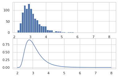
Using the ildj transformation, we can compute log_prob of programs that invertibly transform samples.
def sample(key):
  x = ppl.random_variable(tfd.Normal(0., 1.))(key)
  return jnp.exp(x / 2.) + 2.
_, ax = plt.subplots(2)
ax[0].hist(jit(vmap(sample))(random.split(random.PRNGKey(0), 1000)),
    bins='auto')
x = jnp.linspace(0, 8, 100)
ax[1].plot(x, jnp.exp(jit(vmap(ppl.log_prob(sample)))(x)))
plt.show()
We can tag intermediate values in a probabilistic program with names and obtain joint sampling and joint log-prob functions.
def sample(key):
  z_key, x_key = random.split(key)
  z = ppl.random_variable(tfd.Normal(0., 1.), name='z')(z_key)
  x = ppl.random_variable(tfd.Normal(z, 1.), name='x')(x_key)
  return x
ppl.joint_sample(sample)(random.PRNGKey(0))
{'x': DeviceArray(-1.1076484, dtype=float32),
 'z': DeviceArray(0.14389044, dtype=float32)}
Oryx also has a joint_log_prob function that composes log_prob with joint_sample.
ppl.joint_log_prob(sample)(dict(x=0., z=0.))
DeviceArray(-1.837877, dtype=float32)
To learn more, see the documentation.
Layer 2: Mini-libraries
Building further on top of the layers that handle state and probabilistic programming, Oryx provides experimental mini-libraries tailored for specific applications like deep learning and Bayesian inference.
Neural networks
In oryx.experimental.nn, Oryx provides a set of common neural network Layers that fit neatly into the state API. These layers are built for single examples (not batches) but override batch behaviors to handle patterns like running averages in batch normalization. They also enable passing keyword arguments like training=True/False into modules.
Layers are initialized from a Template like nn.Dense(200) using state.init.
layer = state.init(nn.Dense(200))(random.PRNGKey(0), jnp.zeros(50))
print(layer, layer.params.kernel.shape, layer.params.bias.shape)
Dense(200) (50, 200) (200,)
A Layer has a call method that runs its forward pass.
layer.call(jnp.ones(50)).shape
(200,)
Oryx also provides a Serial combinator.
mlp_template = nn.Serial([
  nn.Dense(200), nn.Relu(),
  nn.Dense(200), nn.Relu(),
  nn.Dense(10), nn.Softmax()
])
# OR
mlp_template = (
    nn.Dense(200) >> nn.Relu()
    >> nn.Dense(200) >> nn.Relu()
    >> nn.Dense(10) >> nn.Softmax())
mlp = state.init(mlp_template)(random.PRNGKey(0), jnp.ones(784))
mlp(jnp.ones(784))
DeviceArray([0.16362445, 0.21150257, 0.14715882, 0.10425295, 0.05952952,
             0.07531884, 0.08368199, 0.0376978 , 0.0159679 , 0.10126514],            dtype=float32)
We can interleave functions and combinators to create a flexible neural network "meta language".
def resnet(template):
  def forward(x, init_key=None):
    layer = state.init(template, name='layer')(init_key, x)
    return x + layer(x)
  return forward

big_resnet_template = nn.Serial([
  nn.Dense(50)
  >> resnet(nn.Dense(50) >> nn.Relu())
  >> resnet(nn.Dense(50) >> nn.Relu())
  >> nn.Dense(10)
])
network = state.init(big_resnet_template)(random.PRNGKey(0), jnp.ones(784))
network(jnp.ones(784))
DeviceArray([-0.03828401,  0.9046303 ,  1.6083915 , -0.17005858,
              3.889552  ,  1.7427744 , -1.0567027 ,  3.0192878 ,
              0.28983995,  1.7103616 ], dtype=float32)
Optimizers
In oryx.experimental.optimizers, Oryx provides a set of first-order optimizers, built using the state API. Their design is based off of JAX's optix library, where optimizers maintain state about a set of gradient updates. Oryx's version manages state using the state API.
network_key, opt_key = random.split(random.PRNGKey(0))
def autoencoder_loss(network, x):
  return jnp.square(network.call(x) - x).mean()
network = state.init(nn.Dense(200) >> nn.Relu() >> nn.Dense(2))(network_key, jnp.zeros(2))
opt = state.init(optimizers.adam(1e-4))(opt_key, network, network)
g = grad(autoencoder_loss)(network, jnp.zeros(2))

g, opt = opt.call_and_update(network, g)
network = optimizers.optix.apply_updates(network, g)
Markov chain Monte Carlo
In oryx.experimental.mcmc, Oryx provides a set of Markov Chain Monte Carlo (MCMC) kernels. MCMC is an approach to approximate Bayesian inference where we draw samples from a Markov chain whose stationary distribution is the posterior distribution of interest.
Oryx's MCMC library builds on both the state and ppl API.
def model(key):
  return jnp.exp(ppl.random_variable(tfd.MultivariateNormalDiag(
      jnp.zeros(2), jnp.ones(2)))(key))
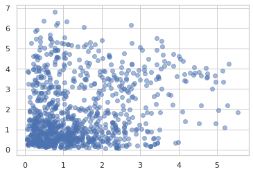
Random walk Metropolis
samples = jit(mcmc.sample_chain(mcmc.metropolis(
    ppl.log_prob(model),
    mcmc.random_walk()), 1000))(random.PRNGKey(0), jnp.ones(2))
plt.scatter(samples[:, 0], samples[:, 1], alpha=0.5)
plt.show()
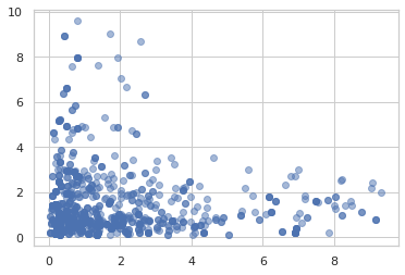
Hamiltonian Monte Carlo
samples = jit(mcmc.sample_chain(mcmc.hmc(
    ppl.log_prob(model)), 1000))(random.PRNGKey(0), jnp.ones(2))
plt.scatter(samples[:, 0], samples[:, 1], alpha=0.5)
plt.show()