Berikut ini penjelasan semantik operasi yang ditetapkan di antarmuka
XlaBuilder. Biasanya, operasi ini memetakan one-to-one ke operasi yang ditentukan dalam antarmuka RPC di xla_data.proto.
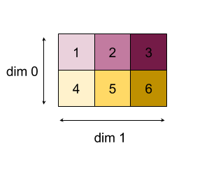
Catatan tentang nomenklatur: jenis data umum yang ditangani XLA adalah array N dimensi yang berisi elemen dari beberapa jenis seragam (seperti float 32-bit). Di seluruh dokumentasi, array digunakan untuk menunjukkan array dimensi arbitrer. Untuk memudahkan, kasus khusus memiliki nama yang lebih spesifik dan sudah dikenal; misalnya vektor adalah array 1 dimensi dan matriks adalah array 2 dimensi.
AfterAll
Lihat juga
XlaBuilder::AfterAll.
AfterAll mengambil sejumlah token token dan menghasilkan satu token. Token adalah jenis primitif yang dapat di-thread antara operasi efek samping untuk menerapkan pengurutan. AfterAll dapat digunakan sebagai gabungan token untuk mengurutkan operasi setelah operasi yang ditetapkan.
AfterAll(operands)
| Argumen | Jenis | Semantik |
|---|---|---|
operands |
XlaOp |
jumlah token variadic |
AllGather
Lihat juga
XlaBuilder::AllGather.
Melakukan penyambungan di seluruh replika.
AllGather(operand, all_gather_dim, shard_count, replica_group_ids,
channel_id)
| Argumen | Jenis | Semantik |
|---|---|---|
operand
|
XlaOp
|
Array untuk menyambungkan seluruh replika |
all_gather_dim |
int64 |
Dimensi penyambungan |
replica_groups
|
vektor vektor
int64 |
Grup di mana penggabungan dilakukan |
channel_id
|
int64 opsional
|
ID saluran opsional untuk komunikasi lintas modul |
replica_groupsadalah daftar grup replika tempat penggabungan dilakukan (ID replika untuk replika saat ini dapat diambil menggunakanReplicaId). Urutan replika dalam setiap grup menentukan urutan inputnya dalam hasil.replica_groupsharus kosong (dalam hal ini semua replika dimiliki oleh satu grup, diurutkan dari0hinggaN - 1), atau berisi jumlah elemen yang sama dengan jumlah replika. Misalnya,replica_groups = {0, 2}, {1, 3}melakukan penyambungan antara replika0dan2, serta1dan3.shard_countadalah ukuran setiap grup replika. Kita memerlukannya jikareplica_groupskosong.channel_iddigunakan untuk komunikasi lintas modul: hanya operasiall-gatherdenganchannel_idyang sama yang dapat saling berkomunikasi.
Bentuk output adalah bentuk input dengan all_gather_dim yang dibuat shard_count
kali lebih besar. Misalnya, jika ada dua replika dan operand memiliki nilai [1.0, 2.5] dan [3.0, 5.25] masing-masing pada kedua replika, nilai output dari operasi ini dengan all_gather_dim 0 akan menjadi [1.0, 2.5, 3.0,
5.25] di kedua replika.
AllReduce
Lihat juga
XlaBuilder::AllReduce.
Melakukan komputasi kustom di seluruh replika.
AllReduce(operand, computation, replica_group_ids, channel_id)
| Argumen | Jenis | Semantik |
|---|---|---|
operand
|
XlaOp
|
Array atau tuple array yang tidak kosong untuk direduksi di berbagai replika |
computation |
XlaComputation |
Komputasi pengurangan |
replica_groups
|
vektor vektor
int64 |
Grup di mana pengurangan dilakukan |
channel_id
|
int64 opsional
|
ID saluran opsional untuk komunikasi lintas modul |
- Jika
operandadalah tuple array, semua pengurangan akan dilakukan pada setiap elemen tuple. replica_groupsadalah daftar grup replika tempat pengurangan dilakukan (ID replika untuk replika saat ini dapat diambil menggunakanReplicaId).replica_groupsharus kosong (jika semua replika dimiliki satu grup), atau berisi jumlah elemen yang sama dengan jumlah replika. Misalnya,replica_groups = {0, 2}, {1, 3}melakukan pengurangan antara replika0dan2, serta1dan3.channel_iddigunakan untuk komunikasi lintas modul: hanya operasiall-reducedenganchannel_idyang sama yang dapat saling berkomunikasi.
Bentuk output sama dengan bentuk input. Misalnya, jika ada dua
replika dan operand memiliki nilai [1.0, 2.5] dan [3.0, 5.25]
masing-masing di dua replika, nilai output dari komputasi
op dan penjumlahan ini akan menjadi [4.0, 7.75] di kedua replika. Jika inputnya adalah
tuple, output-nya juga merupakan tuple.
Menghitung hasil AllReduce memerlukan satu input dari setiap replika,
jadi jika satu replika mengeksekusi node AllReduce lebih kali daripada yang lain, replika
sebelumnya akan menunggu selamanya. Karena semua replika menjalankan program yang sama, tidak banyak cara yang dapat dilakukan. Namun, ada kemungkinan jika kondisi loop bergantung pada data dari infeed dan data yang dimasukkan menyebabkan loop sementara melakukan iterasi lebih sering pada satu replika daripada yang lainnya.
AllToAll
Lihat juga
XlaBuilder::AllToAll.
AllToAll adalah operasi kolektif yang mengirimkan data dari semua core ke semua core. Ini memiliki dua fase:
- Fase pencar. Pada setiap core, operand dibagi menjadi
split_countjumlah blok di sepanjangsplit_dimensions, dan blok tersebut tersebar ke semua core, misalnya, blok ith dikirim ke core i. - Fase pengumpulan. Setiap inti menggabungkan blok yang diterima di sepanjang
concat_dimension.
Core yang berpartisipasi dapat dikonfigurasi dengan:
replica_groups: setiap ReplicaGroup berisi daftar ID replika yang berpartisipasi dalam komputasi (ID replika untuk replika saat ini dapat diambil menggunakanReplicaId). AllToAll akan diterapkan dalam subgrup sesuai urutan yang ditentukan. Misalnya,replica_groups = { {1,2,3}, {4,5,0} }berarti AllToAll akan diterapkan dalam replika{1, 2, 3}, dan dalam fase pengumpulan, dan blok yang diterima akan digabungkan dalam urutan yang sama, yaitu 1, 2, 3. Kemudian, AllToAll lainnya akan diterapkan dalam replika 4, 5, 0, dan urutan penyambungannya juga 4, 5, 0. Jikareplica_groupskosong, semua replika dimiliki oleh satu grup, dalam urutan penyambungan tampilannya.
Prasyarat:
- Ukuran dimensi operand pada
split_dimensiondapat dibagi dengansplit_count. - Bentuk operand bukan tuple.
AllToAll(operand, split_dimension, concat_dimension, split_count,
replica_groups)
| Argumen | Jenis | Semantik |
|---|---|---|
operand |
XlaOp |
array input n dimensi |
split_dimension
|
int64
|
Nilai dalam interval [0,
n) yang memberi nama dimensi
bersama operand yang
dipisah |
concat_dimension
|
int64
|
Nilai dalam interval [0,
n) yang memberi nama dimensi
dan blok pemisahan
digabungkan |
split_count
|
int64
|
Jumlah core yang
berpartisipasi dalam operasi ini. Jika
replica_groups kosong, nilai ini
harus menunjukkan jumlah
replika; jika tidak, jumlah ini harus sama dengan jumlah
replika dalam setiap grup. |
replica_groups
|
Vektor ReplicaGroup
|
Setiap grup berisi daftar ID replika. |
Di bawah ini menunjukkan contoh Alltoall.
XlaBuilder b("alltoall");
auto x = Parameter(&b, 0, ShapeUtil::MakeShape(F32, {4, 16}), "x");
AllToAll(x, /*split_dimension=*/1, /*concat_dimension=*/0, /*split_count=*/4);
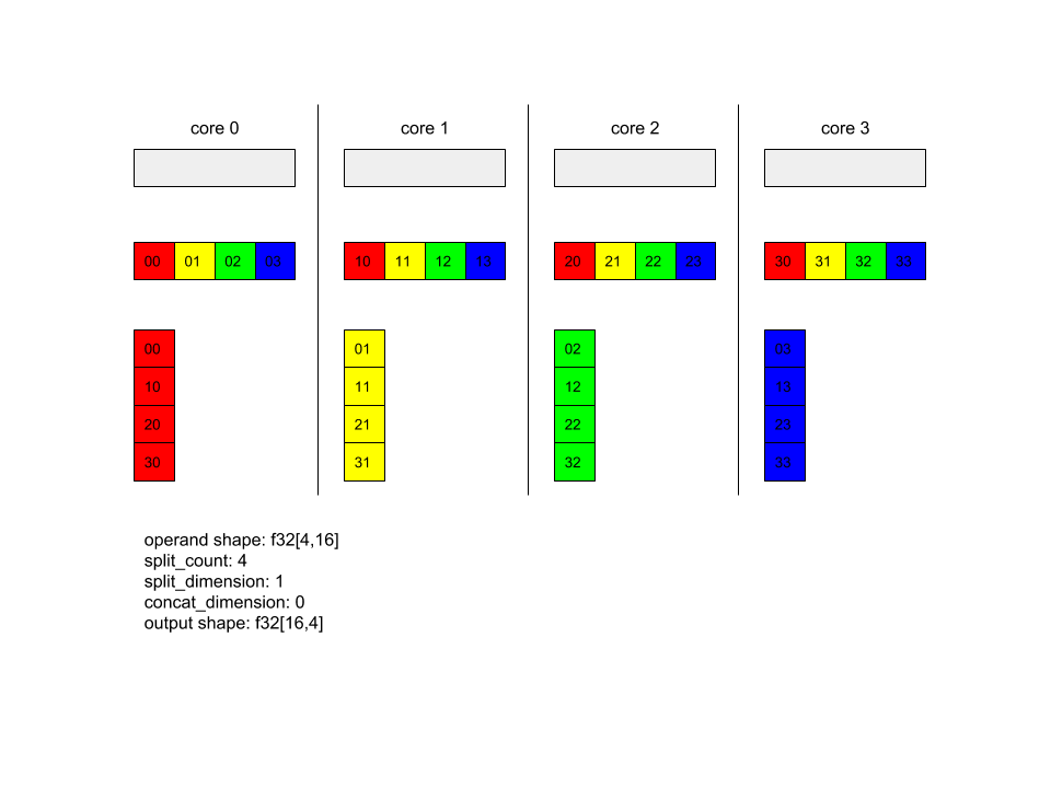
Dalam contoh ini, ada 4 core yang berpartisipasi dalam Alltoall. Pada setiap inti, operan dibagi menjadi 4 bagian di sepanjang dimensi 0, sehingga setiap bagian memiliki bentuk f32[4,4]. Keempat bagian tersebut tersebar ke semua core. Kemudian setiap inti menggabungkan bagian yang diterima di sepanjang dimensi 1, dalam urutan inti 0-4. Jadi {i>output<i} pada setiap inti memiliki bentuk f32[16,4].
BatchNormGrad
Lihat juga
XlaBuilder::BatchNormGrad
dan kertas normalisasi batch asli
untuk mengetahui deskripsi mendetail tentang algoritme.
Menghitung gradien norma tumpukan.
BatchNormGrad(operand, scale, mean, variance, grad_output, epsilon, feature_index)
| Argumen | Jenis | Semantik |
|---|---|---|
operand |
XlaOp |
array dimensi n yang akan dinormalisasi (x) |
scale |
XlaOp |
Array 1 dimensi (\(\gamma\)) |
mean |
XlaOp |
Array 1 dimensi (\(\mu\)) |
variance |
XlaOp |
Array 1 dimensi (\(\sigma^2\)) |
grad_output |
XlaOp |
Gradien yang diteruskan ke BatchNormTraining (\(\nabla y\)) |
epsilon |
float |
Nilai epsilon (\(\epsilon\)) |
feature_index |
int64 |
Indeks ke dimensi fitur di operand |
Untuk setiap fitur dalam dimensi fitur (feature_index adalah indeks untuk dimensi fitur dalam operand), operasi akan menghitung gradien yang sesuai dengan operand, offset, dan scale di semua dimensi lainnya. feature_index harus berupa indeks yang valid untuk dimensi fitur di operand.
Ketiga gradien ditentukan oleh formula berikut (dengan asumsi array 4 dimensi sebagai operand dan dengan indeks dimensi fitur l, ukuran batch m, serta ukuran spasial w dan h):
\[ \begin{split} c_l&= \frac{1}{mwh}\sum_{i=1}^m\sum_{j=1}^w\sum_{k=1}^h \left( \nabla y_{ijkl} \frac{x_{ijkl} - \mu_l}{\sigma^2_l+\epsilon} \right) \\\\ d_l&= \frac{1}{mwh}\sum_{i=1}^m\sum_{j=1}^w\sum_{k=1}^h \nabla y_{ijkl} \\\\ \nabla x_{ijkl} &= \frac{\gamma_{l} }{\sqrt{\sigma^2_{l}+\epsilon} } \left( \nabla y_{ijkl} - d_l - c_l (x_{ijkl} - \mu_{l}) \right) \\\\ \nabla \gamma_l &= \sum_{i=1}^m\sum_{j=1}^w\sum_{k=1}^h \left( \nabla y_{ijkl} \frac{x_{ijkl} - \mu_l}{\sqrt{\sigma^2_{l}+\epsilon} } \right) \\\\\ \nabla \beta_l &= \sum_{i=1}^m\sum_{j=1}^w\sum_{k=1}^h \nabla y_{ijkl} \end{split} \]
Input mean dan variance mewakili nilai momen di seluruh dimensi batch dan
spasial.
Jenis output-nya adalah tuple dari tiga handle:
| Output | Jenis | Semantik |
|---|---|---|
grad_operand
|
XlaOp
|
gradien terhadap input operand ($\nabla
x$) |
grad_scale
|
XlaOp
|
gradien terhadap input scale ($\nabla
\gamma$) |
grad_offset
|
XlaOp
|
gradien terhadap input offset($\nabla
\beta$) |
BatchNormInference
Lihat juga
XlaBuilder::BatchNormInference
dan kertas normalisasi batch asli
untuk mengetahui deskripsi mendetail tentang algoritme.
Menormalisasi array di seluruh dimensi spasi dan batch.
BatchNormInference(operand, scale, offset, mean, variance, epsilon, feature_index)
| Argumen | Jenis | Semantik |
|---|---|---|
operand |
XlaOp |
array dimensi n yang akan dinormalisasi |
scale |
XlaOp |
Array 1 dimensi |
offset |
XlaOp |
Array 1 dimensi |
mean |
XlaOp |
Array 1 dimensi |
variance |
XlaOp |
Array 1 dimensi |
epsilon |
float |
Nilai Epsilon |
feature_index |
int64 |
Indeks ke dimensi fitur di operand |
Untuk setiap fitur dalam dimensi fitur (feature_index adalah indeks untuk dimensi fitur di operand), operasi tersebut menghitung rata-rata dan varians di semua dimensi lainnya dan menggunakan rata-rata dan varian untuk menormalisasi setiap elemen di operand. feature_index harus berupa indeks yang valid untuk dimensi fitur di operand.
BatchNormInference setara dengan memanggil BatchNormTraining tanpa
menghitung mean dan variance untuk setiap batch. Diagram ini menggunakan input mean dan
variance sebagai estimasi nilai. Tujuan dari operasi ini adalah untuk mengurangi latensi dalam inferensi, oleh karena itu dinamakan BatchNormInference.
Outputnya berupa array n dimensi yang dinormalisasi dengan bentuk yang sama seperti operand input.
BatchNormTraining
Lihat juga
XlaBuilder::BatchNormTraining
dan the original batch normalization paper
untuk mengetahui deskripsi mendetail tentang algoritme.
Menormalisasi array di seluruh dimensi spasi dan batch.
BatchNormTraining(operand, scale, offset, epsilon, feature_index)
| Argumen | Jenis | Semantik |
|---|---|---|
operand |
XlaOp |
array dimensi n yang akan dinormalisasi (x) |
scale |
XlaOp |
Array 1 dimensi (\(\gamma\)) |
offset |
XlaOp |
Array 1 dimensi (\(\beta\)) |
epsilon |
float |
Nilai epsilon (\(\epsilon\)) |
feature_index |
int64 |
Indeks ke dimensi fitur di operand |
Untuk setiap fitur dalam dimensi fitur (feature_index adalah indeks untuk dimensi fitur di operand), operasi tersebut menghitung rata-rata dan varians di semua dimensi lainnya dan menggunakan rata-rata dan varian untuk menormalisasi setiap elemen di operand. feature_index harus berupa indeks yang valid untuk dimensi fitur di operand.
Algoritme berjalan sebagai berikut untuk setiap batch di operand \(x\) yang berisi elemen m dengan w dan h sebagai ukuran dimensi spasial (dengan asumsi operand adalah array 4 dimensi):
Menghitung rata-rata batch \(\mu_l\) untuk setiap fitur
ldalam dimensi fitur: \(\mu_l=\frac{1}{mwh}\sum_{i=1}^m\sum_{j=1}^w\sum_{k=1}^h x_{ijkl}\)Menghitung varians batch \(\sigma^2_l\): $\sigma^2l=\frac{1}{mwh}\sum{i=1}^m\sum{j=1}^w\sum{k=1}^h (x_{ijkl} - \mu_l)^2$
Menormalisasi, menskalakan, dan bergeser: \(y_{ijkl}=\frac{\gamma_l(x_{ijkl}-\mu_l)}{\sqrt[2]{\sigma^2_l+\epsilon} }+\beta_l\)
Nilai epsilon, biasanya angka kecil, ditambahkan untuk menghindari kesalahan pembagian dengan nol.
Jenis output adalah tuple dari tiga XlaOp:
| Output | Jenis | Semantik |
|---|---|---|
output
|
XlaOp
|
array n dimensi dengan bentuk yang sama seperti input operand (y) |
batch_mean |
XlaOp |
Array 1 dimensi (\(\mu\)) |
batch_var |
XlaOp |
Array 1 dimensi (\(\sigma^2\)) |
batch_mean dan batch_var adalah momen yang dihitung di seluruh dimensi batch dan spasial menggunakan formula di atas.
BitcastConvertType
Lihat juga
XlaBuilder::BitcastConvertType.
Serupa dengan tf.bitcast di TensorFlow, melakukan operasi bitcast berdasarkan elemen dari bentuk data ke bentuk target. Ukuran input dan output harus
cocok: misalnya elemen s32 menjadi elemen f32 melalui rutinitas bitcast, dan satu
elemen s32 akan menjadi empat elemen s8. Bitcast diimplementasikan sebagai transmisi level rendah, sehingga mesin dengan representasi floating point yang berbeda akan memberikan hasil yang berbeda.
BitcastConvertType(operand, new_element_type)
| Argumen | Jenis | Semantik |
|---|---|---|
operand |
XlaOp |
array jenis T dengan redup D |
new_element_type |
PrimitiveType |
tipe U |
Dimensi operand dan bentuk target harus cocok, terlepas dari dimensi terakhir yang akan berubah berdasarkan rasio ukuran dasar sebelum dan setelah konversi.
Jenis elemen sumber dan tujuan tidak boleh berupa tupel.
Mengonversi bitcast ke jenis primitif dengan lebar yang berbeda
Petunjuk HLO BitcastConvert mendukung kasus ketika ukuran jenis elemen
output T' tidak sama dengan ukuran elemen input T. Karena
seluruh operasi secara konseptual merupakan bitcast dan tidak mengubah byte
yang mendasarinya, bentuk elemen output harus berubah. Untuk B = sizeof(T), B' =
sizeof(T'), ada dua kemungkinan kasus.
Pertama, saat B > B', bentuk output mendapatkan dimensi minor baru dari ukuran B/B'. Contoh:
f16[10,2]{1,0} %output = f16[10,2]{1,0} bitcast-convert(f32[10]{0} %input)
Aturannya tetap sama untuk skalar efektif:
f16[2]{0} %output = f16[2]{0} bitcast-convert(f32[] %input)
Atau, untuk B' > B, petunjuk mengharuskan dimensi logika terakhir
dari bentuk input harus sama dengan B'/B, dan dimensi ini dihapus selama
konversi:
f32[10]{0} %output = f32[10]{0} bitcast-convert(f16[10,2]{1,0} %input)
Perhatikan bahwa konversi antara bitwidth yang berbeda tidak bersifat elementwise.
Siarkan
Lihat juga
XlaBuilder::Broadcast.
Menambahkan dimensi ke array dengan menduplikasi data dalam array.
Broadcast(operand, broadcast_sizes)
| Argumen | Jenis | Semantik |
|---|---|---|
operand |
XlaOp |
Array yang akan diduplikasi |
broadcast_sizes |
ArraySlice<int64> |
Ukuran dimensi baru |
Dimensi baru disisipkan di sebelah kiri, yaitu jika broadcast_sizes memiliki
nilai {a0, ..., aN} dan bentuk operand memiliki dimensi {b0, ..., bM},
bentuk output memiliki dimensi {a0, ..., aN, b0, ..., bM}.
Indeks dimensi baru ke dalam salinan operand, yaitu
output[i0, ..., iN, j0, ..., jM] = operand[j0, ..., jM]
Misalnya, jika operand adalah f32 skalar dengan nilai 2.0f, dan
broadcast_sizes adalah {2, 3}, hasilnya adalah array dengan bentuk
f32[2, 3] dan semua nilai dalam hasilnya adalah 2.0f.
BroadcastInDim
Lihat juga
XlaBuilder::BroadcastInDim.
Memperluas ukuran dan peringkat array dengan menduplikasi data dalam array.
BroadcastInDim(operand, out_dim_size, broadcast_dimensions)
| Argumen | Jenis | Semantik |
|---|---|---|
operand |
XlaOp |
Array yang akan diduplikasi |
out_dim_size |
ArraySlice<int64> |
Ukuran dimensi bentuk target |
broadcast_dimensions |
ArraySlice<int64> |
Dimensi mana dalam bentuk target yang sesuai dengan setiap dimensi bentuk operand |
Mirip dengan Broadcast, tetapi memungkinkan penambahan dimensi di mana saja dan memperluas dimensi yang ada dengan ukuran 1.
operand disiarkan ke bentuk yang dijelaskan oleh out_dim_size.
broadcast_dimensions memetakan dimensi operand ke dimensi
bentuk target, yaitu dimensi ke-i operand dipetakan ke dimensi
broadcast_dimension[i] dari bentuk output. Dimensi
operand harus memiliki ukuran 1 atau sama ukurannya dengan dimensi dalam bentuk
output yang dipetakan. Dimensi yang tersisa diisi dengan dimensi
ukuran 1. Penyiaran dimensi merosot, lalu menyiarkan bersama dimensi
yang merosot ini untuk mencapai bentuk output. Semantik ini dijelaskan secara mendetail di
halaman penyiaran.
Panggilan Telepon
Lihat juga
XlaBuilder::Call.
Memanggil komputasi dengan argumen yang diberikan.
Call(computation, args...)
| Argumen | Jenis | Semantik |
|---|---|---|
computation |
XlaComputation |
komputasi jenis T_0, T_1, ..., T_{N-1} -> S dengan parameter N dari jenis arbitrer |
args |
urutan N XlaOpd |
Argumen N jenis arbitrer |
Aritas dan jenis args harus cocok dengan parameter
computation. Diperbolehkan untuk tidak memiliki args.
Kolesky
Lihat juga
XlaBuilder::Cholesky.
Menghitung dekomposisi Cholesky dari batch matriks pasti positif simetris (Hermitian).
Cholesky(a, lower)
| Argumen | Jenis | Semantik |
|---|---|---|
a |
XlaOp |
array peringkat > 2 dari jenis kompleks atau floating point. |
lower |
bool |
apakah akan menggunakan segitiga atas atau bawah a. |
Jika lower adalah true, menghitung matriks segitiga lebih rendah l sedemikian rupa sehingga $a = l .
l^T$. Jika lower adalah false, akan menghitung matriks segitiga atas u sedemikian rupa sehingga
\(a = u^T . u\).
Data input hanya dibaca dari segitiga bawah/atas a, bergantung pada
nilai lower. Nilai dari segitiga lainnya akan diabaikan. Data output
ditampilkan dalam segitiga yang sama; nilai dalam segitiga lainnya
ditentukan oleh implementasi dan bisa berupa apa saja.
Jika peringkat a lebih besar dari 2, a akan diperlakukan sebagai batch matriks,
dengan semua dimensi kecuali 2 minor adalah dimensi batch.
Jika a tidak simetris (Hermitian) positif pasti, hasilnya adalah
ditentukan implementasi.
Penjepit
Lihat juga
XlaBuilder::Clamp.
Menjepit operand ke dalam rentang antara nilai minimum dan maksimum.
Clamp(min, operand, max)
| Argumen | Jenis | Semantik |
|---|---|---|
min |
XlaOp |
array jenis T |
operand |
XlaOp |
array jenis T |
max |
XlaOp |
array jenis T |
Dengan mempertimbangkan operand dan nilai minimum dan maksimum, tampilkan operand jika operand berada dalam
rentang antara minimum dan maksimum, jika tidak, nilai minimum akan ditampilkan jika
operand berada di bawah rentang ini, atau nilai maksimum jika operand berada di atas rentang
ini. Artinya, clamp(a, x, b) = min(max(a, x), b).
Ketiga array harus memiliki bentuk yang sama. Atau, sebagai bentuk terbatas
penyiaran, min dan/atau max dapat menjadi skalar berjenis T.
Contoh dengan skalar min dan max:
let operand: s32[3] = {-1, 5, 9};
let min: s32 = 0;
let max: s32 = 6;
==>
Clamp(min, operand, max) = s32[3]{0, 5, 6};
Ciutkan
Lihat juga
operasi XlaBuilder::Collapse
dan tf.reshape.
Menciutkan dimensi array menjadi satu dimensi.
Collapse(operand, dimensions)
| Argumen | Jenis | Semantik |
|---|---|---|
operand |
XlaOp |
array jenis T |
dimensions |
Vektor int64 |
{i>subset<i} dimensi T yang berurutan dan berurutan. |
Ciutkan menggantikan subset dimensi operand yang diberikan dengan satu
dimensi. Argumen input adalah array arbitrer dari jenis T dan
vektor konstanta waktu kompilasi indeks dimensi. Indeks dimensi harus
berurutan (bilangan dimensi rendah ke tinggi), subset dimensi
T yang berurutan. Dengan demikian, {0, 1, 2}, {0, 1}, atau {1, 2} adalah kumpulan dimensi yang valid, tetapi
{1, 0} atau {0, 2} tidak valid. Dimensi tersebut diganti dengan satu dimensi baru, pada posisi yang sama dalam urutan dimensi seperti saat dimensi diganti, dengan ukuran dimensi baru yang sama dengan produk ukuran dimensi asli. Jumlah dimensi
terendah di dimensions adalah dimensi dengan variasi paling lambat (paling utama)
di tingkatan loop yang menciutkan dimensi ini, dan jumlah dimensi
tertinggi bervariasi paling cepat (paling kecil). Lihat operator tf.reshape jika pengurutan penciutan yang lebih umum diperlukan.
Misalnya, biarkan v menjadi array dari 24 elemen:
let v = f32[4x2x3] { { {10, 11, 12},  {15, 16, 17} },
{ {20, 21, 22},  {25, 26, 27} },
{ {30, 31, 32},  {35, 36, 37} },
{ {40, 41, 42},  {45, 46, 47} } };

// Collapse to a single dimension, leaving one dimension.
let v012 = Collapse(v, {0,1,2});
then v012 == f32[24] {10, 11, 12, 15, 16, 17,
20, 21, 22, 25, 26, 27,
30, 31, 32, 35, 36, 37,
40, 41, 42, 45, 46, 47};

// Collapse the two lower dimensions, leaving two dimensions.
let v01 = Collapse(v, {0,1});
then v01 == f32[4x6] { {10, 11, 12, 15, 16, 17},
{20, 21, 22, 25, 26, 27},
{30, 31, 32, 35, 36, 37},
{40, 41, 42, 45, 46, 47} };

// Collapse the two higher dimensions, leaving two dimensions.
let v12 = Collapse(v, {1,2});
then v12 == f32[8x3] { {10, 11, 12},
{15, 16, 17},
{20, 21, 22},
{25, 26, 27},
{30, 31, 32},
{35, 36, 37},
{40, 41, 42},
{45, 46, 47} };
CollectivePermute
Lihat juga
XlaBuilder::CollectivePermute.
CollectivePermute adalah operasi kolektif yang mengirim dan menerima replikasi silang data.
CollectivePermute(operand, source_target_pairs)
| Argumen | Jenis | Semantik |
|---|---|---|
operand |
XlaOp |
array input n dimensi |
source_target_pairs |
Vektor <int64, int64> |
Daftar pasangan (source_replica_id, target_replica_id). Untuk setiap pasangan, operand dikirim dari replika sumber ke replika target. |
Perhatikan bahwa ada pembatasan berikut di source_target_pair:
- Dua pasangan tidak boleh memiliki ID replika target yang sama dan tidak boleh memiliki ID replika sumber yang sama.
- Jika ID replika bukan target dalam pasangan apa pun, output pada replika tersebut adalah tensor yang terdiri dari 0 dengan bentuk yang sama dengan inputnya.
Gabungkan
Lihat juga
XlaBuilder::ConcatInDim.
Penyambungan akan menyusun array dari beberapa operand array. Array memiliki peringkat yang sama dengan setiap operand array input (yang harus berperingkat sama satu sama lain) dan berisi argumen dalam urutan yang ditentukan.
Concatenate(operands..., dimension)
| Argumen | Jenis | Semantik |
|---|---|---|
operands |
urutan dari N XlaOp |
Array N dari jenis T dengan dimensi [L0, L1, ...]. Membutuhkan N >= 1. |
dimension |
int64 |
Nilai dalam interval [0, N) yang memberi nama dimensi yang akan digabungkan di antara operands. |
Kecuali dimension, semua dimensi harus sama. Hal ini karena XLA tidak mendukung array "ragged". Perhatikan juga bahwa nilai peringkat 0 tidak dapat digabungkan (karena tidak mungkin untuk memberi nama dimensi tempat terjadinya penyambungan).
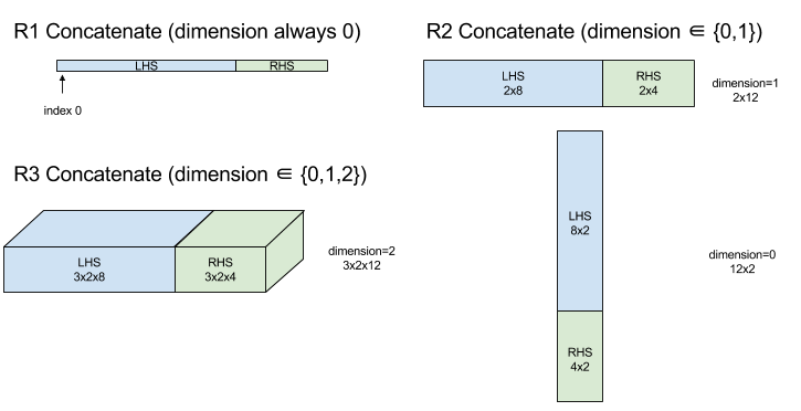
Contoh 1 dimensi:
Concat({ {2, 3}, {4, 5}, {6, 7} }, 0)
>>> {2, 3, 4, 5, 6, 7}
Contoh 2 dimensi:
let a = {
{1, 2},
{3, 4},
{5, 6},
};
let b = {
{7, 8},
};
Concat({a, b}, 0)
>>> {
{1, 2},
{3, 4},
{5, 6},
{7, 8},
}
Diagram:
Kondisional
Lihat juga
XlaBuilder::Conditional.
Conditional(pred, true_operand, true_computation, false_operand,
false_computation)
| Argumen | Jenis | Semantik |
|---|---|---|
pred |
XlaOp |
Skalar jenis PRED |
true_operand |
XlaOp |
Argumen jenis \(T_0\) |
true_computation |
XlaComputation |
XlaKomputasi jenis \(T_0 \to S\) |
false_operand |
XlaOp |
Argumen jenis \(T_1\) |
false_computation |
XlaComputation |
XlaKomputasi jenis \(T_1 \to S\) |
Mengeksekusi true_computation jika pred adalah true, false_computation jika pred
adalah false, dan menampilkan hasilnya.
true_computation harus menggunakan satu argumen dari jenis \(T_0\) dan akan
dipanggil dengan true_operand yang harus berjenis sama. false_computation
harus menggunakan satu argumen dari jenis \(T_1\) dan akan
dipanggil dengan false_operand yang harus berjenis sama. Jenis
nilai yang ditampilkan true_computation dan false_computation harus sama.
Perhatikan bahwa hanya satu dari true_computation dan false_computation yang akan
dieksekusi, bergantung pada nilai pred.
Conditional(branch_index, branch_computations, branch_operands)
| Argumen | Jenis | Semantik |
|---|---|---|
branch_index |
XlaOp |
Skalar jenis S32 |
branch_computations |
urutan dari N XlaComputation |
XlaComputasi dari jenis \(T_0 \to S , T_1 \to S , ..., T_{N-1} \to S\) |
branch_operands |
urutan dari N XlaOp |
Argumen jenis \(T_0 , T_1 , ..., T_{N-1}\) |
Mengeksekusi branch_computations[branch_index], dan menampilkan hasilnya. Jika
branch_index adalah S32 yang < 0 atau >= N, branch_computations[N-1]
akan dieksekusi sebagai cabang default.
Setiap branch_computations[b] harus menggunakan satu argumen dari jenis \(T_b\) dan
akan dipanggil dengan branch_operands[b] yang harus berjenis sama. Jenis
nilai yang ditampilkan dari setiap branch_computations[b] harus sama.
Perhatikan bahwa hanya satu dari branch_computations yang akan dieksekusi, bergantung pada
nilai branch_index.
Konv (konvolusi)
Lihat juga
XlaBuilder::Conv.
Sebagai ConvWithGeneralPadding, tetapi padding ditentukan dengan singkat sebagai
SAMA atau VALID. Padding SAME melapisi input (lhs) dengan angka nol, sehingga
output memiliki bentuk yang sama dengan input ketika tidak mempertimbangkan
langkah melangkah. Padding VALID berarti tidak ada padding.
ConvWithGeneralPadding (konvolusi)
Lihat juga
XlaBuilder::ConvWithGeneralPadding.
Menghitung konvolusi jenis yang digunakan dalam jaringan neural. Di sini, konvolusi dapat dianggap sebagai jendela n-dimensi yang bergerak melintasi area dasar n-dimensi dan komputasi dilakukan untuk setiap kemungkinan posisi jendela.
| Argumen | Jenis | Semantik |
|---|---|---|
lhs |
XlaOp |
peringkat n+2 array input |
rhs |
XlaOp |
peringkat n+2 array bobot kernel |
window_strides |
ArraySlice<int64> |
Array n-d dari langkah kernel |
padding |
ArraySlice< pair<int64,int64>> |
array n-d padding (rendah, tinggi) |
lhs_dilation |
ArraySlice<int64> |
Array faktor dilatasi n-d ls |
rhs_dilation |
ArraySlice<int64> |
Array faktor dilatasi n-d rhs |
feature_group_count |
int64 | jumlah grup fitur |
batch_group_count |
int64 | jumlah kelompok batch |
Misalkan n adalah jumlah dimensi spasial. Argumen lhs adalah array peringkat n+2 yang mendeskripsikan area dasar. Ini disebut input, meskipun tentu saja
rhs juga merupakan input. Dalam jaringan neural, ini adalah aktivasi input.
Dimensi n+2, dalam urutan ini:
batch: Setiap koordinat dalam dimensi ini mewakili input independen yang digunakan untuk konvolusi.z/depth/features: Setiap posisi (y,x) di area dasar memiliki vektor yang terkait dengannya, yang masuk ke dimensi ini.spatial_dims: Menjelaskan dimensi spasialnyang menentukan area dasar tempat jendela bergerak.
Argumen rhs adalah array peringkat n+2 yang menjelaskan filter/kernel/jendela konvolusional. Dimensi tersebut, dalam urutan ini:
output-z: Dimensizoutput.input-z: Ukuran dimensi ini dikalifeature_group_countharus sama dengan ukuran dimensizdalam lb.spatial_dims: Menjelaskan dimensi spasialnyang menentukan jendela n-d yang bergerak di seluruh area dasar.
Argumen window_strides menentukan langkah jendela konvolusional
dalam dimensi spasial. Misalnya, jika langkah dalam dimensi spasial pertama
adalah 3, jendela hanya dapat ditempatkan pada koordinat dengan
indeks spasial pertama yang habis dibagi 3.
Argumen padding menentukan jumlah padding nol yang akan diterapkan ke
area dasar. Jumlah padding bisa negatif -- nilai absolut
padding negatif menunjukkan jumlah elemen yang akan dihapus dari dimensi
yang ditentukan sebelum melakukan konvolusi. padding[0] menentukan padding untuk
dimensi y dan padding[1] menentukan padding untuk dimensi x. Setiap
pasangan memiliki padding rendah sebagai elemen pertama dan padding tinggi sebagai elemen
kedua. Padding rendah diterapkan ke arah indeks bawah, sedangkan padding tinggi diterapkan ke arah indeks yang lebih tinggi. Misalnya, jika padding[1] adalah (2,3), akan ada padding dengan 2 angka nol di sebelah kiri dan dengan 3 angka nol di sebelah kanan dalam dimensi spasial kedua. Menggunakan padding
sama dengan memasukkan nilai nol yang sama tersebut ke dalam input (lhs) sebelum
melakukan konvolusi.
Argumen lhs_dilation dan rhs_dilation menentukan faktor dilatasi yang akan
diterapkan ke ls dan rhs, di setiap dimensi spasial. Jika faktor dilatasi dalam dimensi spasial adalah d, lubang d-1 secara implisit ditempatkan di antara setiap entri dalam dimensi tersebut, sehingga ukuran array akan bertambah. Lubang diisi dengan nilai tanpa pengoperasian, yang untuk konvolusi berarti nol.
Pelebaran rhs juga disebut konvolusi yang mengerikan. Untuk detail selengkapnya, lihat
tf.nn.atrous_conv2d. Dilatasi Ls juga disebut
konvolusi {i>transpose<i}. Untuk detail selengkapnya, lihat tf.nn.conv2d_transpose.
Argumen feature_group_count (nilai default 1) dapat digunakan untuk konvolusi yang dikelompokkan. feature_group_count harus menjadi pembagi dari dimensi fitur input dan output. Jika feature_group_count lebih besar dari 1, artinya secara konseptual dimensi fitur input dan output serta dimensi fitur output rhs dibagi secara merata menjadi banyak grup feature_group_count, yang masing-masing grup terdiri dari suburutan fitur yang berurutan. Dimensi
fitur input rhs harus sama dengan dimensi fitur input
lhs dibagi dengan feature_group_count (sehingga sudah memiliki ukuran
grup fitur input). Grup ke-i digunakan bersama untuk menghitung
feature_group_count untuk banyak konvolusi yang terpisah. Hasil konvolusi ini digabungkan bersama dalam dimensi fitur output.
Untuk konvolusi kedalaman, argumen feature_group_count akan ditetapkan ke dimensi fitur input, dan filter akan dibentuk ulang dari [filter_height, filter_width, in_channels, channel_multiplier] menjadi [filter_height, filter_width, 1, in_channels * channel_multiplier]. Untuk mengetahui detail
selengkapnya, lihat tf.nn.depthwise_conv2d.
Argumen batch_group_count (nilai default 1) dapat digunakan untuk filter yang dikelompokkan selama propagasi mundur. batch_group_count harus menjadi pembagi
ukuran dimensi batch lhs (input). Jika batch_group_count lebih besar
dari 1, berarti dimensi batch output harus berukuran input batch
/ batch_group_count. batch_group_count harus menjadi pembagi ukuran fitur
output.
Bentuk output memiliki dimensi berikut, dalam urutan ini:
batch: Ukuran dimensi ini dikalibatch_group_countharus sama dengan ukuran dimensibatchdalam j.z: Ukuran yang sama sepertioutput-zpada kernel (rhs).spatial_dims: Satu nilai untuk setiap penempatan jendela konvolusional yang valid.

Gambar di atas menunjukkan cara kerja kolom batch_group_count. Secara efektif, kita
membagi setiap batch nahs menjadi grup batch_group_count, dan melakukan hal yang sama untuk
fitur output. Kemudian, untuk setiap grup ini, kita melakukan konvolusi berpasangan dan menggabungkan output di sepanjang dimensi fitur output. Semantik operasional
semua dimensi lainnya (fitur dan spasial) tetap sama.
Penempatan jendela konvolusional yang valid ditentukan oleh langkah dan ukuran area dasar setelah padding.
Untuk mendeskripsikan fungsi konvolusi, pertimbangkan konvolusi 2d, dan pilih beberapa koordinat batch, z, y, x yang tetap dalam output. Kemudian, (y,x) adalah
posisi sudut jendela dalam area dasar (mis. sudut kiri atas,
bergantung pada cara Anda menafsirkan dimensi spasial). Kita sekarang memiliki jendela 2d, yang diambil dari area dasar, dengan setiap titik 2d dikaitkan dengan vektor
1d, sehingga kita mendapatkan kotak 3d. Dari kernel konvolusional, karena kita telah menetapkan
koordinat output z, kita juga memiliki kotak 3d. Kedua kotak tersebut memiliki dimensi
yang sama, jadi kita bisa menjumlahkan perkalian dengan unsur-unsur di antara kedua
kotak tersebut (serupa dengan perkalian titik). Itulah nilai output.
Perlu diketahui bahwa jika output-z misalnya, 5, maka setiap posisi jendela akan menghasilkan 5
nilai dalam output ke dimensi z output. Nilai-nilai ini berbeda
di bagian mana dari kernel konvolusional yang digunakan - ada kotak nilai 3d
terpisah yang digunakan untuk setiap koordinat output-z. Jadi Anda bisa menganggapnya sebagai 5
konvolusi terpisah dengan filter berbeda untuk masing-masingnya.
Berikut adalah kode semu untuk konvolusi 2d dengan padding dan striding:
for (b, oz, oy, ox) {  // output coordinates
  value = 0;
  for (iz, ky, kx) {  // kernel coordinates and input z
    iy = oy*stride_y + ky - pad_low_y;
    ix = ox*stride_x + kx - pad_low_x;
    if ((iy, ix) inside the base area considered without padding) {
      value += input(b, iz, iy, ix) * kernel(oz, iz, ky, kx);
    }
  }
  output(b, oz, oy, ox) = value;
}
ConvertElementType
Lihat juga
XlaBuilder::ConvertElementType.
Serupa dengan static_cast berbasis elemen di C++, menjalankan operasi konversi
berbasis elemen dari bentuk data ke bentuk target. Dimensi harus
cocok, dan konversinya harus berbasis elemen; misalnya, elemen s32 menjadi
elemen f32 melalui rutinitas konversi s32 ke f32.
ConvertElementType(operand, new_element_type)
| Argumen | Jenis | Semantik |
|---|---|---|
operand |
XlaOp |
array jenis T dengan redup D |
new_element_type |
PrimitiveType |
tipe U |
Dimensi operand dan bentuk target harus cocok. Jenis elemen sumber dan tujuan tidak boleh berupa tupel.
Konversi seperti T=s32 ke U=f32 akan melakukan rutinitas konversi int-to-float
yang menormalisasi seperti pembulatan ke nilai terdekat genap.
let a: s32[3] = {0, 1, 2};
let b: f32[3] = convert(a, f32);
then b == f32[3]{0.0, 1.0, 2.0}
CrossReplicaSum
Melakukan AllReduce dengan komputasi penjumlahan.
CustomCall
Lihat juga
XlaBuilder::CustomCall.
Memanggil fungsi yang disediakan pengguna dalam komputasi.
CustomCall(target_name, args..., shape)
| Argumen | Jenis | Semantik |
|---|---|---|
target_name |
string |
Nama fungsi. Petunjuk panggilan akan dikeluarkan yang menargetkan nama simbol ini. |
args |
urutan N XlaOpd |
N argumen jenis arbitrer, yang akan diteruskan ke fungsi. |
shape |
Shape |
Bentuk output fungsi |
Tanda tangan fungsi sama, terlepas dari aritas atau jenis argumen:
extern "C" void target_name(void* out, void** in);
Misalnya, jika CustomCall digunakan sebagai berikut:
let x = f32[2] {1,2};
let y = f32[2x3] { {10, 20, 30}, {40, 50, 60} };

CustomCall("myfunc", {x, y}, f32[3x3])
Berikut adalah contoh implementasi myfunc:
extern "C" void myfunc(void* out, void** in) {
  float (&x)[2] = *static_cast<float(*)[2]>(in[0]);
  float (&y)[2][3] = *static_cast<float(*)[2][3]>(in[1]);
  EXPECT_EQ(1, x[0]);
  EXPECT_EQ(2, x[1]);
  EXPECT_EQ(10, y[0][0]);
  EXPECT_EQ(20, y[0][1]);
  EXPECT_EQ(30, y[0][2]);
  EXPECT_EQ(40, y[1][0]);
  EXPECT_EQ(50, y[1][1]);
  EXPECT_EQ(60, y[1][2]);
  float (&z)[3][3] = *static_cast<float(*)[3][3]>(out);
  z[0][0] = x[1] + y[1][0];
  // ...
}
Fungsi yang diberikan pengguna tidak boleh memiliki efek samping dan eksekusinya harus idempoten.
Titik
Lihat juga
XlaBuilder::Dot.
Dot(lhs, rhs)
| Argumen | Jenis | Semantik |
|---|---|---|
lhs |
XlaOp |
array jenis T |
rhs |
XlaOp |
array jenis T |
Semantik persis operasi ini bergantung pada peringkat operand:
| Input | Output | Semantik |
|---|---|---|
vektor [n] vektor dot [n] |
skalar | perkalian titik vektor |
matriks [m x k] vektor dot [k] |
vektor [m] | perkalian matriks-vektor |
matriks [m x k] dot matriks [k x n] |
matriks [m x n] | perkalian matriks-matriks |
Operasi tersebut menjalankan jumlah perkalian pada dimensi kedua lhs (atau
yang pertama jika memiliki peringkat 1) dan dimensi pertama rhs. Ini adalah dimensi
"terkontrak". Dimensi terkontrak lhs dan rhs harus
berukuran sama. Dalam praktiknya, AI generatif dapat digunakan untuk melakukan perkalian titik di antara vektor, perkalian vektor/matriks, atau perkalian matriks/matriks.
DotGeneral
Lihat juga
XlaBuilder::DotGeneral.
DotGeneral(lhs, rhs, dimension_numbers)
| Argumen | Jenis | Semantik |
|---|---|---|
lhs |
XlaOp |
array jenis T |
rhs |
XlaOp |
array jenis T |
dimension_numbers |
DotDimensionNumbers |
nomor dimensi batch dan kontrak |
Serupa dengan Dot, tetapi memungkinkan nomor dimensi kontrak dan batch ditentukan untuk lhs dan rhs.
| Kolom DotDimensionNumbers | Jenis | Semantik |
|---|---|---|
lhs_contracting_dimensions
|
int64 berulang | lhs nomor dimensi
mengontrak |
rhs_contracting_dimensions
|
int64 berulang | rhs nomor dimensi
mengontrak |
lhs_batch_dimensions
|
int64 berulang | lhs nomor dimensi
batch |
rhs_batch_dimensions
|
int64 berulang | rhs nomor dimensi
batch |
DotGeneral melakukan jumlah produk dibandingkan dimensi kontrak yang ditentukan dalam
dimension_numbers.
Angka dimensi terkontrak terkait dari lhs dan rhs tidak harus
sama tetapi harus memiliki ukuran dimensi yang sama.
Contoh dengan nomor dimensi kontrak:
lhs = { {1.0, 2.0, 3.0},
{4.0, 5.0, 6.0} }

rhs = { {1.0, 1.0, 1.0},
{2.0, 2.0, 2.0} }

DotDimensionNumbers dnums;
dnums.add_lhs_contracting_dimensions(1);
dnums.add_rhs_contracting_dimensions(1);

DotGeneral(lhs, rhs, dnums) -> { {6.0, 12.0},
{15.0, 30.0} }
Nomor dimensi batch terkait dari lhs dan rhs harus memiliki ukuran dimensi
yang sama.
Contoh dengan nomor dimensi batch (ukuran tumpukan 2, matriks 2x2):
lhs = { { {1.0, 2.0},
{3.0, 4.0} },
{ {5.0, 6.0},
{7.0, 8.0} } }

rhs = { { {1.0, 0.0},
{0.0, 1.0} },
{ {1.0, 0.0},
{0.0, 1.0} } }

DotDimensionNumbers dnums;
dnums.add_lhs_contracting_dimensions(2);
dnums.add_rhs_contracting_dimensions(1);
dnums.add_lhs_batch_dimensions(0);
dnums.add_rhs_batch_dimensions(0);

DotGeneral(lhs, rhs, dnums) -> { { {1.0, 2.0},
{3.0, 4.0} },
{ {5.0, 6.0},
{7.0, 8.0} } }
| Input | Output | Semantik |
|---|---|---|
[b0, m, k] dot [b0, k, n] |
[b0, b, n] | matmul batch |
[b0, b1, m, k] dot [b0, b1, k, n] |
[b0, b1, m, n] | matmul batch |
Dengan demikian, nomor dimensi yang dihasilkan dimulai dengan dimensi batch,
lalu dimensi non-kontrak/non-batch lhs, dan terakhir dimensi
non-kontrak/non-batch rhs.
DynamicSlice
Lihat juga
XlaBuilder::DynamicSlice.
DynamicSlice mengekstrak sub-array dari array input pada start_indices dinamis. Ukuran irisan di setiap dimensi diteruskan dalam
size_indices, yang menentukan titik akhir interval irisan eksklusif di setiap
dimensi: [awal, awal + ukuran). Bentuk start_indices harus berperingkat ==
1, dengan ukuran dimensi sama dengan peringkat operand.
DynamicSlice(operand, start_indices, size_indices)
| Argumen | Jenis | Semantik |
|---|---|---|
operand |
XlaOp |
Array dimensi N jenis T |
start_indices |
urutan dari N XlaOp |
Daftar bilangan bulat skalar N yang berisi indeks awal irisan untuk setiap dimensi. Nilai harus lebih besar atau sama dengan nol. |
size_indices |
ArraySlice<int64> |
Daftar bilangan bulat N yang berisi ukuran irisan untuk setiap dimensi. Setiap nilai harus benar-benar lebih besar dari nol, dan ukuran awal + harus kurang dari atau sama dengan ukuran dimensi untuk menghindari penggabungan ukuran dimensi modulus. |
Indeks irisan efektif dihitung dengan menerapkan transformasi
berikut untuk setiap indeks i di [1, N) sebelum menjalankan slice:
start_indices[i] = clamp(start_indices[i], 0, operand.dimension_size[i] - size_indices[i])
Hal ini memastikan bahwa slice yang diekstrak selalu dalam terikat sehubungan dengan array operand. Jika slice berada di dalam sebelum transformasi diterapkan, transformasi tidak akan berpengaruh.
Contoh 1 dimensi:
let a = {0.0, 1.0, 2.0, 3.0, 4.0}
let s = {2}

DynamicSlice(a, s, {2}) produces:
{2.0, 3.0}
Contoh 2 dimensi:
let b =
{ {0.0,  1.0,  2.0},
{3.0,  4.0,  5.0},
{6.0,  7.0,  8.0},
{9.0, 10.0, 11.0} }
let s = {2, 1}

DynamicSlice(b, s, {2, 2}) produces:
{ { 7.0,  8.0},
{10.0, 11.0} }
DynamicUpdateSlice
Lihat juga
XlaBuilder::DynamicUpdateSlice.
DynamicUpdateSlice menghasilkan hasil yang merupakan nilai array input operand, dengan irisan update yang ditimpa di start_indices.
Bentuk update menentukan bentuk sub-array hasil yang
diupdate.
Bentuk start_indices harus berperingkat == 1, dengan ukuran dimensi yang sama dengan
peringkat operand.
DynamicUpdateSlice(operand, update, start_indices)
| Argumen | Jenis | Semantik |
|---|---|---|
operand |
XlaOp |
Array dimensi N jenis T |
update |
XlaOp |
Array dimensi N jenis T yang berisi pembaruan irisan. Setiap dimensi bentuk update harus lebih besar dari nol, dan start + update harus kurang dari atau sama dengan ukuran operand untuk setiap dimensi agar tidak menghasilkan indeks update di luar batas. |
start_indices |
urutan dari N XlaOp |
Daftar bilangan bulat skalar N yang berisi indeks awal irisan untuk setiap dimensi. Nilai harus lebih besar atau sama dengan nol. |
Indeks irisan efektif dihitung dengan menerapkan transformasi
berikut untuk setiap indeks i di [1, N) sebelum menjalankan slice:
start_indices[i] = clamp(start_indices[i], 0, operand.dimension_size[i] - update.dimension_size[i])
Hal ini memastikan bahwa slice yang diperbarui selalu dalam batasan sehubungan dengan array Operand. Jika slice berada di dalam sebelum transformasi diterapkan, transformasi tidak akan berpengaruh.
Contoh 1 dimensi:
let a = {0.0, 1.0, 2.0, 3.0, 4.0}
let u = {5.0, 6.0}
let s = {2}

DynamicUpdateSlice(a, u, s) produces:
{0.0, 1.0, 5.0, 6.0, 4.0}
Contoh 2 dimensi:
let b =
{ {0.0,  1.0,  2.0},
{3.0,  4.0,  5.0},
{6.0,  7.0,  8.0},
{9.0, 10.0, 11.0} }
let u =
{ {12.0,  13.0},
{14.0,  15.0},
{16.0,  17.0} }

let s = {1, 1}

DynamicUpdateSlice(b, u, s) produces:
{ {0.0,  1.0,  2.0},
{3.0, 12.0, 13.0},
{6.0, 14.0, 15.0},
{9.0, 16.0, 17.0} }
Operasi aritmatika biner {i>element<i}-{i>wise<i}
Lihat juga
XlaBuilder::Add.
Mendukung serangkaian operasi aritmatika biner berbasis elemen.
Op(lhs, rhs)
Dengan Op adalah salah satu dari Add (penambahan), Sub (pengurangan), Mul
(perkalian), Div (pembagian), Rem (sisa), Max (maksimum), Min
(minimum), LogicalAnd (AND logis), atau LogicalOr (log logis).
| Argumen | Jenis | Semantik |
|---|---|---|
lhs |
XlaOp |
operand kiri: array jenis T |
rhs |
XlaOp |
operand kanan: array jenis T |
Bentuk argumen harus mirip atau kompatibel. Lihat dokumentasi penyiaran tentang apa artinya kompatibel dengan bentuk. Hasil operasi memiliki bentuk yang merupakan hasil dari penyiaran dua array input. Dalam varian ini, operasi antar-array dengan peringkat yang berbeda tidak didukung, kecuali jika salah satu operand adalah skalar.
Jika Op adalah Rem, tanda hasil diambil dari dividen, dan nilai absolut hasilnya selalu lebih kecil dari nilai absolut pembagi.
Overflow pembagian bilangan bulat (pembagian/sisa yang ditandatangani/tidak ditandatangani dengan nol atau pembagian/sisa
yang ditandatangani dari INT_SMIN dengan -1) menghasilkan nilai yang ditentukan
implementasi.
Terdapat varian alternatif dengan dukungan penyiaran dengan tingkat yang berbeda untuk operasi berikut:
Op(lhs, rhs, broadcast_dimensions)
Dengan Op sama dengan yang di atas. Varian operasi ini harus digunakan untuk operasi aritmetika antara array dengan peringkat yang berbeda (seperti menambahkan matriks ke vektor).
Operand broadcast_dimensions tambahan adalah bagian bilangan bulat yang digunakan untuk
memperluas peringkat operand dengan peringkat lebih rendah ke peringkat operand
yang lebih tinggi. broadcast_dimensions memetakan dimensi bentuk berperingkat lebih rendah ke dimensi bentuk berperingkat lebih tinggi. Dimensi yang tidak dipetakan dari bentuk yang diperluas
diisi dengan dimensi ukuran satu. Penyiaran dimensi menurun
lalu menyiarkan bentuk di sepanjang dimensi yang merosot ini untuk menyamakan
bentuk kedua operand. Semantik ini dijelaskan secara mendetail di
halaman penyiaran.
Operasi perbandingan {i>element<i}-{i>wise<i}
Lihat juga
XlaBuilder::Eq.
Kumpulan operasi perbandingan biner standar yang memperhitungkan elemen didukung. Perhatikan bahwa semantik perbandingan floating point IEEE 754 standar berlaku saat membandingkan jenis floating point.
Op(lhs, rhs)
Dengan Op adalah salah satu dari Eq (sama dengan), Ne (tidak sama dengan), Ge
(lebih besar atau sama dari), Gt (lebih besar dari), Le (kurang atau sama dengan), Lt
(kurang-dari). Kumpulan operator lainnya, EqTotalOrder, NeTotalOrder, GeTotalOrder, GtTotalOrder, LeTotalOrder, dan LtTotalOrder, memberikan fungsi yang sama, kecuali bahwa operator tersebut juga mendukung urutan total pada bilangan floating point, dengan menerapkan -NaN < -Inf < -Finite < -0 < +0 < +Finite <Na
| Argumen | Jenis | Semantik |
|---|---|---|
lhs |
XlaOp |
operand kiri: array jenis T |
rhs |
XlaOp |
operand kanan: array jenis T |
Bentuk argumen harus mirip atau kompatibel. Lihat
dokumentasi penyiaran tentang apa artinya kompatibel
dengan bentuk. Hasil operasi memiliki bentuk yang merupakan hasil dari
penyiaran dua array input dengan jenis elemen PRED. Dalam varian ini,
operasi antara array dengan peringkat yang berbeda tidak didukung, kecuali jika salah satu
operand adalah skalar.
Terdapat varian alternatif dengan dukungan penyiaran dengan tingkat yang berbeda untuk operasi berikut:
Op(lhs, rhs, broadcast_dimensions)
Dengan Op sama dengan yang di atas. Varian operasi ini harus digunakan untuk operasi perbandingan antara array dengan peringkat yang berbeda (seperti menambahkan matriks ke vektor).
Operand broadcast_dimensions tambahan adalah bagian bilangan bulat yang menentukan
dimensi yang akan digunakan untuk menyiarkan operand. Semantik dijelaskan
secara mendetail di halaman penyiaran.
Fungsi unary yang {i>element<i}-{i>wise<i}
XlaBuilder mendukung fungsi unary berbasis elemen ini:
Abs(operand) absen berbasis elemen x -> |x|.
Ceil(operand) Ceil berbasis elemen x -> ⌈x⌉.
Cos(operand) Kosinus x -> cos(x) berdasarkan elemen.
Exp(operand) x -> e^x eksponensial alami berbasis elemen.
Floor(operand) Lantai berdasarkan elemen x -> ⌊x⌋.
Imag(operand) Bagian imajiner dari elemen yang kompleks (atau nyata). x -> imag(x). Jika operand adalah tipe floating point, menampilkan 0.
IsFinite(operand) Menguji apakah setiap elemen operand terbatas,
artinya, bukan tak terbatas positif atau negatif, dan bukan NaN. Menampilkan array nilai PRED dengan bentuk yang sama seperti input, dengan setiap elemen bernilai true jika dan hanya jika elemen input yang sesuai terbatas.
Log(operand) Logaritma alami berbasis elemen x -> ln(x).
LogicalNot(operand) Logika element-wise, bukan x -> !(x).
Logistic(operand) Komputasi fungsi logistik berbasis elemen x ->
logistic(x).
PopulationCount(operand) Menghitung jumlah bit yang ditetapkan dalam setiap
elemen operand.
Neg(operand) negasi berbasis elemen x -> -x.
Real(operand) Bagian nyata berbasis elemen dari bentuk kompleks (atau nyata).
x -> real(x). Jika operand adalah jenis floating point, akan menampilkan nilai yang sama.
Rsqrt(operand) Kebalikan elemen dari operasi akar kuadrat x -> 1.0 / sqrt(x).
Sign(operand) Operasi tanda {i>element<i}-wise x -> sgn(x) dengan
\[\text{sgn}(x) = \begin{cases} -1 & x < 0\\ -0 & x = -0\\ NaN & x = NaN\\ +0 & x = +0\\ 1 & x > 0 \end{cases}\]
menggunakan operator perbandingan jenis elemen operand.
Sqrt(operand) Operasi akar kuadrat berbasis elemen x -> sqrt(x).
Cbrt(operand) Operasi akar kubik berbasis elemen x -> cbrt(x).
Tanh(operand) Tangen hiperbolik berbasis elemen x -> tanh(x).
Round(operand) Pembulatan berbasis elemen, mengikat menjauh dari nol.
RoundNearestEven(operand) Pembulatan berbasis elemen, mengikat ke bilangan genap terdekat.
| Argumen | Jenis | Semantik |
|---|---|---|
operand |
XlaOp |
Operand ke fungsi |
Fungsi ini diterapkan ke setiap elemen dalam array operand, sehingga menghasilkan array dengan bentuk yang sama. operand diizinkan untuk menjadi skalar (peringkat 0).
Fft
Operasi XLA FFT mengimplementasikan Transformasi Fourier maju dan terbalik untuk input/output yang nyata dan kompleks. FFT multidimensi pada maksimal 3 sumbu didukung.
Lihat juga
XlaBuilder::Fft.
| Argumen | Jenis | Semantik |
|---|---|---|
operand |
XlaOp |
Array yang akan kita transformasikan Fourier. |
fft_type |
FftType |
Lihat tabel di bawah. |
fft_length |
ArraySlice<int64> |
Panjang domain waktu sumbu yang diubah. Hal ini diperlukan khususnya agar IRFFT dapat menyesuaikan ukuran sumbu terdalam, karena RFFT(fft_length=[16]) memiliki bentuk output yang sama dengan RFFT(fft_length=[17]). |
FftType |
Semantik |
|---|---|
FFT |
Meneruskan FFT kompleks ke kompleks. Bentuk tidak berubah. |
IFFT |
FFT kompleks ke kompleks terbalik. Bentuk tidak berubah. |
RFFT |
Meneruskan FFT real-ke-kompleks. Bentuk sumbu terdalam dikurangi menjadi fft_length[-1] // 2 + 1 jika fft_length[-1] bukan nilai nol, sehingga menghilangkan bagian konjugasi terbalik dari sinyal yang diubah di luar frekuensi Nyquist. |
IRFFT |
FFT real-ke-kompleks terbalik (yaitu mengambil kompleks, menampilkan real). Bentuk sumbu terdalam diperluas menjadi fft_length[-1] jika fft_length[-1] adalah nilai bukan nol, yang menyimpulkan bagian sinyal yang diubah di luar frekuensi Nyquist dari konjugasi terbalik entri 1 ke fft_length[-1] // 2 + 1. |
FFT Multidimensi
Jika lebih dari 1 fft_length disediakan, hal ini setara dengan menerapkan
operasi FFT ke setiap sumbu terdalam. Perhatikan bahwa untuk
kasus nyata yang nyata> kompleks dan kompleks, transformasi sumbu terdalam
(secara efektif) dilakukan terlebih dahulu (RFFT; terakhir untuk IRFFT), itulah sebabnya sumbu
terdalam adalah yang mengubah ukuran. Transformasi sumbu lainnya akan
menjadi kompleks->kompleks.
Detail implementasi
CPU FFT didukung oleh TensorFFT Eigen. GPU FFT menggunakan cuFFT.
Kumpulkan
Operasi pengumpulan XLA menggabungkan beberapa irisan (setiap irisan pada offset runtime yang mungkin berbeda) dari array input.
Semantik Umum
Lihat juga
XlaBuilder::Gather.
Untuk deskripsi yang lebih intuitif, lihat bagian "Deskripsi Informal" di bawah.
gather(operand, start_indices, offset_dims, collapsed_slice_dims, slice_sizes, start_index_map)
| Argumen | Jenis | Semantik |
|---|---|---|
operand |
XlaOp |
Array yang kita kumpulkan. |
start_indices |
XlaOp |
Array yang berisi indeks awal dari irisan yang kita kumpulkan. |
index_vector_dim |
int64 |
Dimensi dalam start_indices yang "berisi" indeks awal. Lihat di bawah untuk deskripsi mendetail. |
offset_dims |
ArraySlice<int64> |
Kumpulan dimensi dalam bentuk output yang di-offset ke dalam array yang diiris dari operand. |
slice_sizes |
ArraySlice<int64> |
slice_sizes[i] adalah batas untuk bagian pada dimensi i. |
collapsed_slice_dims |
ArraySlice<int64> |
Kumpulan dimensi di setiap irisan yang diciutkan. Dimensi ini harus memiliki ukuran 1. |
start_index_map |
ArraySlice<int64> |
Peta yang menjelaskan cara memetakan indeks di start_indices ke indeks hukum ke dalam operand. |
indices_are_sorted |
bool |
Apakah indeks dijamin akan diurutkan oleh pemanggil. |
unique_indices |
bool |
Apakah indeks dijamin unik oleh pemanggil. |
Untuk memudahkan, kami melabeli dimensi dalam array output, bukan dalam offset_dims sebagai batch_dims.
Output-nya adalah array peringkat batch_dims.size + offset_dims.size.
operand.rank harus sama dengan jumlah offset_dims.size dan
collapsed_slice_dims.size. Selain itu, slice_sizes.size harus sama dengan
operand.rank.
Jika index_vector_dim sama dengan start_indices.rank, secara implisit kami menganggap
start_indices memiliki dimensi 1 di akhir (yaitu, jika start_indices memiliki
bentuk [6,7] dan index_vector_dim adalah 2, secara implisit kami menganggap
bentuk start_indices sebagai [6,7,1]).
Batas untuk array output di sepanjang dimensi i dihitung sebagai berikut:
Jika
iada dibatch_dims(yaitu sama denganbatch_dims[k]untuk beberapak), kami memilih batas dimensi yang sesuai daristart_indices.shape, melewatiindex_vector_dim(yaitu pilihstart_indices.shape.dims[k] jikak<index_vector_dimdanstart_indices.shape.dims[k+1] sebaliknya).Jika
iada dioffset_dims(yaitu sama denganoffset_dims[k] untuk beberapak), kita memilih batas yang sesuai darislice_sizessetelah memperhitungkancollapsed_slice_dims(yaitu, kita memilihadjusted_slice_sizes[k] denganadjusted_slice_sizesslice_sizesdengan batas pada indekscollapsed_slice_dimsdihapus).
Secara formal, indeks operand In yang sesuai dengan indeks output yang diberikan Out
dihitung sebagai berikut:
Biarkan
G= {Out[k] untukkdalambatch_dims}. GunakanGuntuk membagi vektorSsehinggaS[i] =start_indices[Gabungkan(G,i)] tempat Gabungkan(A, b) menyisipkan b pada posisiindex_vector_dimke A. Perhatikan bahwa hal ini ditentukan dengan baik meskipunGkosong: JikaGkosong, makaS=start_indices.Buat indeks awal,
Sin, keoperandmenggunakanSdengan menyebarkanSmenggunakanstart_index_map. Lebih tepatnya:Sin[start_index_map[k]] =S[k] jikak<start_index_map.size.Sin[_] =0jika sebaliknya.
Buat indeks
Oinkeoperanddengan menyebarkan indeks pada dimensi offset diOutsesuai dengancollapsed_slice_dimsyang ditetapkan. Lebih tepatnya:Oin[remapped_offset_dims(k)] =Out[offset_dims[k]] jikak<offset_dims.size(remapped_offset_dimsditentukan di bawah).Oin[_] =0jika sebaliknya.
InadalahOin+Sindengan + adalah penambahan menurut elemen.
remapped_offset_dims adalah fungsi monoton dengan domain [0,
offset_dims.size) dan rentang [0, operand.rank) \ collapsed_slice_dims. Jadi,
jika, misalnya, offset_dims.size adalah 4, operand.rank adalah 6, dan
collapsed_slice_dims adalah {0, 2}, lalu remapped_offset_dims adalah {0→1,
1→3, 2→4, 3→5}.
Jika indices_are_sorted disetel ke benar (true), XLA dapat mengasumsikan bahwa start_indices
diurutkan (dalam urutan start_index_map menaik) oleh pengguna. Jika tidak,
semantik akan ditetapkan.
Jika unique_indices disetel ke benar (true), XLA dapat mengasumsikan bahwa semua elemen
yang tersebar bersifat unik. Jadi XLA dapat menggunakan operasi non-atom. Jika
unique_indices disetel ke benar (true) dan indeks yang tersebar tidak
unik, maka semantik diimplementasikan.
Deskripsi dan Contoh informal
Secara informal, setiap Out indeks dalam array output sesuai dengan elemen E
dalam array operand, yang dihitung sebagai berikut:
Kita menggunakan dimensi batch di
Outuntuk mencari indeks awal daristart_indices.Kita menggunakan
start_index_mapuntuk memetakan indeks awal (yang ukurannya mungkin lebih kecil dari operand.rank) ke indeks awal "penuh" ke dalamoperand.Kita secara dinamis membagi potongan dengan ukuran
slice_sizesmenggunakan indeks awal lengkap.Kita membentuk ulang irisan dengan menciutkan dimensi
collapsed_slice_dims. Karena semua dimensi irisan yang diciutkan harus memiliki batas 1, bentuk ulang ini selalu sah.Kita menggunakan dimensi offset di
Outuntuk mengindeks ke dalam irisan ini guna mendapatkan elemen input,E, yang sesuai dengan indeks outputOut.
index_vector_dim ditetapkan ke start_indices.rank - 1 di semua contoh
berikutnya. Nilai yang lebih menarik untuk index_vector_dim tidak akan mengubah
operasi secara mendasar, tetapi membuat representasi visual menjadi lebih rumit.
Untuk mendapatkan intuisi tentang kecocokan semua hal di atas, mari kita lihat
contoh yang mengumpulkan 5 irisan bentuk [8,6] dari array [16,11]. Posisi
irisan ke dalam array [16,11] dapat direpresentasikan sebagai vektor
indeks bentuk S64[2], sehingga kumpulan 5 posisi dapat direpresentasikan sebagai
array S64[5,2].
Perilaku operasi pengumpulan kemudian dapat digambarkan sebagai transformasi
indeks yang menggunakan [G,O0,O1], sebuah indeks dalam
bentuk output, dan memetakannya ke elemen dalam array input dengan cara
berikut:

Pertama-tama, kita memilih vektor (X,Y) dari array indeks pengumpulan menggunakan G.
Kemudian, elemen dalam array output pada indeks
[G,O0,O1] adalah elemen dalam array input
pada indeks [X+O0,Y+O1].
slice_sizes adalah [8,6], yang menentukan rentang O0 dan
O1, dan selanjutnya menentukan batas irisan tersebut.
Operasi pengumpulan ini bertindak sebagai irisan dinamis batch dengan G sebagai dimensi
batch.
Indeks pengumpulan mungkin multidimensi. Misalnya, versi yang lebih umum dari contoh di atas yang menggunakan array "budaya indeks" dari bentuk [4,5,2] akan menerjemahkan indeks seperti ini:

Sekali lagi, ini berfungsi sebagai irisan dinamis batch G0 dan
G1 sebagai dimensi batch. Ukuran irisan masih [8,6].
Operasi pengumpulan di XLA menggeneralisasi semantik informal yang diuraikan di atas dengan cara berikut:
Kita dapat mengonfigurasi dimensi mana dalam bentuk output yang merupakan dimensi offset (dimensi yang berisi
O0,O1di contoh terakhir). Dimensi batch output (dimensi yang berisiG0,G1di contoh terakhir) ditentukan sebagai dimensi output yang tidak mengimbangi dimensi.Jumlah dimensi offset output yang secara eksplisit ada dalam bentuk output mungkin lebih kecil daripada peringkat input. Dimensi yang "tidak ada" ini, yang dicantumkan secara eksplisit sebagai
collapsed_slice_dims, harus memiliki ukuran irisan1. Karena keduanya memiliki ukuran irisan1, satu-satunya indeks yang valid untuk keduanya adalah0dan mengeluarkannya tidak menimbulkan ambiguitas.Bagian yang diekstrak dari array "Mengumpulkan Indeks" ((
X,Y) pada contoh terakhir) mungkin memiliki lebih sedikit elemen daripada peringkat array input, dan pemetaan eksplisit menentukan bagaimana indeks harus diperluas agar memiliki peringkat yang sama dengan input.
Sebagai contoh terakhir, kita menggunakan (2) dan (3) untuk mengimplementasikan tf.gather_nd:

G0 dan G1 digunakan untuk memisahkan indeks awal dari array indeks pengumpulan seperti biasa, kecuali indeks awal hanya memiliki satu elemen, yaitu X. Demikian pula, hanya ada satu indeks offset output dengan nilai
O0. Namun, sebelum digunakan sebagai indeks ke dalam array input,
nilai ini diperluas sesuai dengan "Kumpulkan Pemetaan Indeks" (start_index_map dalam
deskripsi formal) dan "Pemetaan Offset" (remapped_offset_dims dalam
deskripsi formal) menjadi [X,0] dan [0,O0],
menambahkan hingga [X,O0]. Dengan kata lain, indeks output
[0O] dan O sebagai indeks output
1 dan G1.G0000GGGatherIndicestf.gather_nd
slice_sizes untuk kasus ini adalah [1,11]. Secara intuitif, ini berarti bahwa setiap indeks X dalam array indeks pengumpulan akan memilih seluruh baris dan hasilnya adalah penyambungan dari semua baris tersebut.
GetDimensionSize
Lihat juga
XlaBuilder::GetDimensionSize.
Menampilkan ukuran dimensi yang diberikan dari operand. Operand harus berbentuk array.
GetDimensionSize(operand, dimension)
| Argumen | Jenis | Semantik |
|---|---|---|
operand |
XlaOp |
array input n dimensi |
dimension |
int64 |
Nilai dalam interval [0, n) yang menentukan dimensi |
SetDimensionSize
Lihat juga
XlaBuilder::SetDimensionSize.
Menetapkan ukuran dinamis dimensi yang ditentukan XlaOp. Operand harus berbentuk array.
SetDimensionSize(operand, size, dimension)
| Argumen | Jenis | Semantik |
|---|---|---|
operand |
XlaOp |
n array input dimensi. |
size |
XlaOp |
int32 yang mewakili ukuran dinamis runtime. |
dimension |
int64 |
Nilai dalam interval [0, n) yang menentukan dimensi. |
Teruskan operand sebagai hasil, dengan dimensi dinamis yang dilacak oleh compiler.
Nilai dengan padding akan diabaikan oleh operasi pengurangan downstream.
let v: f32[10] = f32[10]{1, 2, 3, 4, 5, 6, 7, 8, 9, 10};
let five: s32 = 5;
let six: s32 = 6;

// Setting dynamic dimension size doesn't change the upper bound of the static
// shape.
let padded_v_five: f32[10] = set_dimension_size(v, five, /*dimension=*/0);
let padded_v_six: f32[10] = set_dimension_size(v, six, /*dimension=*/0);

// sum == 1 + 2 + 3 + 4 + 5
let sum:f32[] = reduce_sum(padded_v_five);
// product == 1 * 2 * 3 * 4 * 5
let product:f32[] = reduce_product(padded_v_five);

// Changing padding size will yield different result.
// sum == 1 + 2 + 3 + 4 + 5 + 6
let sum:f32[] = reduce_sum(padded_v_six);
GetTupleElement
Lihat juga
XlaBuilder::GetTupleElement.
Mengindeks ke dalam tuple dengan nilai konstanta waktu kompilasi.
Nilai harus berupa konstanta waktu kompilasi sehingga inferensi bentuk dapat menentukan jenis nilai yang dihasilkan.
Ini serupa dengan std::get<int N>(t) di C++. Secara konseptual:
let v: f32[10] = f32[10]{0, 1, 2, 3, 4, 5, 6, 7, 8, 9};
let s: s32 = 5;
let t: (f32[10], s32) = tuple(v, s);
let element_1: s32 = gettupleelement(t, 1);  // Inferred shape matches s32.
Lihat juga tf.tuple.
Dalam Feed
Lihat juga
XlaBuilder::Infeed.
Infeed(shape)
| Argumen | Jenis | Semantik |
|---|---|---|
shape |
Shape |
Bentuk data yang dibaca dari antarmuka Infeed. Kolom tata letak bentuk harus disetel agar sesuai dengan tata letak data yang dikirim ke perangkat; jika tidak, perilakunya tidak ditentukan. |
Membaca satu item data dari antarmuka streaming Infeed implisit
perangkat, menafsirkan data sebagai bentuk tertentu dan tata letaknya, serta menampilkan
XlaOp data. Beberapa operasi Infeed diizinkan dalam
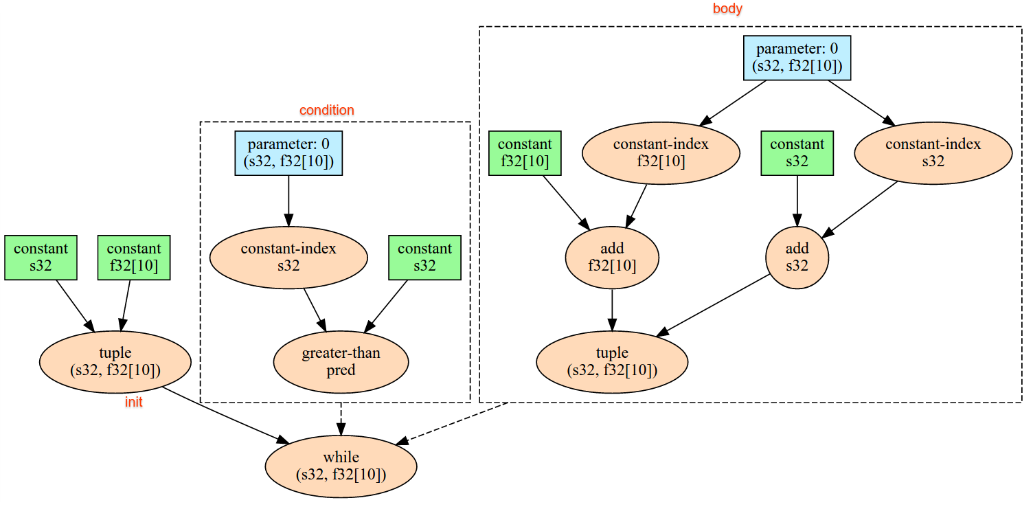
komputasi, tetapi harus ada urutan total di antara operasi Infeed. Misalnya, dua Infeed dalam kode di bawah memiliki total urutan karena ada dependensi di antara loop if.
result1 = while (condition, init = init_value) {
  Infeed(shape)
}

result2 = while (condition, init = result1) {
  Infeed(shape)
}
Bentuk tuple bertingkat tidak didukung. Untuk bentuk tuple kosong, operasi Infeed pada dasarnya adalah tanpa pengoperasian dan dilanjutkan tanpa membaca data apa pun dari Infeed perangkat.
Iota
Lihat juga
XlaBuilder::Iota.
Iota(shape, iota_dimension)
Membangun literal konstan di perangkat, bukan transfer host yang berpotensi
besar. Membuat array yang telah menentukan bentuk dan menyimpan nilai mulai dari nol dan bertambah satu di sepanjang dimensi yang ditentukan. Untuk jenis floating point, array yang dihasilkan setara dengan ConvertElementType(Iota(...)) yang
Iota adalah jenis integral dan konversinya ke jenis floating point.
| Argumen | Jenis | Semantik |
|---|---|---|
shape |
Shape |
Bentuk array yang dibuat oleh Iota() |
iota_dimension |
int64 |
Dimensi yang akan bertambah. |
Misalnya, Iota(s32[4, 8], 0) akan menampilkan
  [[0, 0, 0, 0, 0, 0, 0, 0 ],
   [1, 1, 1, 1, 1, 1, 1, 1 ],
   [2, 2, 2, 2, 2, 2, 2, 2 ],
   [3, 3, 3, 3, 3, 3, 3, 3 ]]
Pengembalian dengan biaya Iota(s32[4, 8], 1)
  [[0, 1, 2, 3, 4, 5, 6, 7 ],
   [0, 1, 2, 3, 4, 5, 6, 7 ],
   [0, 1, 2, 3, 4, 5, 6, 7 ],
   [0, 1, 2, 3, 4, 5, 6, 7 ]]
Peta
Lihat juga
XlaBuilder::Map.
Map(operands..., computation)
| Argumen | Jenis | Semantik |
|---|---|---|
operands |
urutan N XlaOpd |
Array N dari jenis T0..T{N-1} |
computation |
XlaComputation |
komputasi jenis T_0, T_1, .., T_{N + M -1} -> S dengan parameter N jenis T dan M dari jenis arbitrer |
dimensions |
Array int64 |
array dimensi peta |
Menerapkan fungsi skalar pada array operands tertentu, yang menghasilkan array dimensi yang sama yang setiap elemennya merupakan hasil dari fungsi yang dipetakan yang diterapkan pada elemen yang sesuai dalam array input.
Fungsi yang dipetakan adalah komputasi arbitrer dengan batasan bahwa fungsi tersebut memiliki N input jenis skalar T dan satu output dengan jenis S. Output memiliki
dimensi yang sama dengan operand, kecuali jenis elemen T diganti
dengan S.
Misalnya: Map(op1, op2, op3, computation, par1) memetakan elem_out <-
computation(elem1, elem2, elem3, par1) pada setiap indeks (multi-dimensi) dalam
array input untuk menghasilkan array output.
OptimizationBarrier
Memblokir penerusan pengoptimalan apa pun agar tidak memindahkan komputasi melintasi batasan.
Memastikan bahwa semua input dievaluasi sebelum operator yang bergantung pada output penghalang.
Bantalan
Lihat juga
XlaBuilder::Pad.
Pad(operand, padding_value, padding_config)
| Argumen | Jenis | Semantik |
|---|---|---|
operand |
XlaOp |
array jenis T |
padding_value |
XlaOp |
skalar jenis T untuk mengisi padding yang ditambahkan |
padding_config |
PaddingConfig |
jumlah padding di kedua tepi (rendah, tinggi) dan di antara elemen pada setiap dimensi |
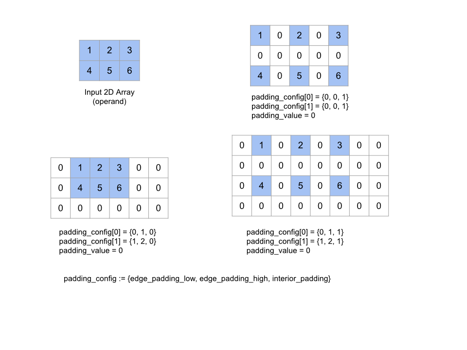
Memperluas array operand yang diberikan dengan padding di sekitar array serta di antara elemen array dengan padding_value yang diberikan. padding_config
menentukan jumlah padding tepi dan padding interior untuk setiap
dimensi.
PaddingConfig adalah kolom berulang PaddingConfigDimension, yang berisi
tiga kolom untuk setiap dimensi: edge_padding_low, edge_padding_high, dan
interior_padding.
edge_padding_low dan edge_padding_high menentukan jumlah padding yang ditambahkan
di bagian bawah (di samping indeks 0) dan kelas atas (di samping indeks tertinggi)
dari setiap dimensi. Jumlah padding tepi bisa negatif --
nilai absolut padding negatif menunjukkan jumlah elemen yang akan dihapus
dari dimensi yang ditentukan.
interior_padding menentukan jumlah padding yang ditambahkan antara dua
elemen di setiap dimensi; jumlah ini tidak boleh negatif. Padding interior terjadi
secara logis sebelum padding tepi, sehingga pada kasus padding tepi negatif, elemen
akan dihapus dari operand dengan padding bagian dalam.
Operasi ini tidak beroperasi jika pasangan padding tepi semuanya (0, 0) dan
nilai padding interior semuanya 0. Gambar di bawah menunjukkan contoh nilai edge_padding dan interior_padding yang berbeda untuk array dua dimensi.
Diterima
Lihat juga
XlaBuilder::Recv.
Recv(shape, channel_handle)
| Argumen | Jenis | Semantik |
|---|---|---|
shape |
Shape |
bentuk data yang akan diterima |
channel_handle |
ChannelHandle |
ID unik untuk setiap pasangan pengirim/penerima |
Menerima data bentuk tertentu dari petunjuk Send dalam komputasi
lain yang memiliki handle saluran yang sama. Menampilkan XlaOp untuk data yang diterima.
API klien dari operasi Recv mewakili komunikasi sinkron.
Namun, petunjuk ini diurai secara internal menjadi 2 petunjuk HLO
(Recv dan RecvDone) untuk memungkinkan transfer data asinkron. Lihat juga
HloInstruction::CreateRecv dan HloInstruction::CreateRecvDone.
Recv(const Shape& shape, int64 channel_id)
Mengalokasikan resource yang diperlukan untuk menerima data dari petunjuk Send dengan channel_id yang sama. Menampilkan konteks untuk resource yang dialokasikan, yang digunakan
oleh petunjuk RecvDone berikut untuk menunggu penyelesaian transfer
data. Konteksnya adalah tuple dari {menerima buffer (bentuk), ID permintaan
(U32)}, dan hanya dapat digunakan oleh petunjuk RecvDone.
RecvDone(HloInstruction context)
Dengan mempertimbangkan konteks yang dibuat oleh petunjuk Recv, menunggu transfer data selesai dan menampilkan data yang diterima.
Reduce (Mengurangi)
Lihat juga
XlaBuilder::Reduce.
Menerapkan fungsi pengurangan ke satu atau beberapa array secara paralel.
Reduce(operands..., init_values..., computation, dimensions)
| Argumen | Jenis | Semantik |
|---|---|---|
operands |
Urutan N XlaOp |
Array N dari jenis T_0, ..., T_{N-1}. |
init_values |
Urutan N XlaOp |
Skalar N jenis T_0, ..., T_{N-1}. |
computation |
XlaComputation |
komputasi jenis T_0, ..., T_{N-1}, T_0, ..., T_{N-1} -> Collate(T_0, ..., T_{N-1}). |
dimensions |
Array int64 |
dimensi yang tidak berurutan. |
Dengan keterangan:
- N harus lebih besar atau sama dengan 1.
- Komputasi harus "secara kasar" asosiatif (lihat di bawah).
- Semua array input harus memiliki dimensi yang sama.
- Semua nilai awal harus membentuk identitas di
computation. - Jika
N = 1,Collate(T)adalahT. - Jika
N > 1,Collate(T_0, ..., T_{N-1})adalah tuple dari elemenNdari jenisT.
Operasi ini mengurangi satu atau beberapa dimensi dari setiap array input menjadi skalar.
Peringkat setiap array yang ditampilkan adalah rank(operand) - len(dimensions). Output
op adalah Collate(Q_0, ..., Q_N) dengan Q_i adalah array jenis T_i, yang
dimensinya dijelaskan di bawah ini.
Backend yang berbeda diizinkan untuk mengaitkan kembali komputasi pengurangan. Hal ini dapat menyebabkan perbedaan numerik, karena beberapa fungsi pengurangan seperti penambahan tidak asosiatif untuk nilai mengambang. Namun, jika rentang data terbatas, penambahan floating point hampir bersifat asosiatif untuk sebagian besar penggunaan praktis.
Contoh
Saat mengurangi satu dimensi dalam array 1D tunggal dengan nilai [10, 11,
12, 13], dengan fungsi pengurangan f (ini adalah computation), hal tersebut dapat dihitung sebagai
f(10, f(11, f(12, f(init_value, 13)))
tetapi ada juga banyak kemungkinan lain, mis.
f(init_value, f(f(10, f(init_value, 11)), f(f(init_value, 12), f(init_value, 13))))
Berikut adalah contoh kasar kode pseudo tentang cara penerapan pengurangan, menggunakan penjumlahan sebagai komputasi pengurangan dengan nilai awal 0.
result_shape <- remove all dims in dimensions from operand_shape

# Iterate over all elements in result_shape. The number of r's here is equal
# to the rank of the result
for r0 in range(result_shape[0]), r1 in range(result_shape[1]), ...:
  # Initialize this result element
  result[r0, r1...] <- 0

  # Iterate over all the reduction dimensions
  for d0 in range(dimensions[0]), d1 in range(dimensions[1]), ...:
    # Increment the result element with the value of the operand's element.
    # The index of the operand's element is constructed from all ri's and di's
    # in the right order (by construction ri's and di's together index over the
    # whole operand shape).
    result[r0, r1...] += operand[ri... di]
Berikut adalah contoh pengurangan array 2D (matriks). Bentuk ini memiliki peringkat 2, dimensi 0 untuk ukuran 2 dan dimensi 1 untuk ukuran 3:
Hasil pengurangan dimensi 0 atau 1 dengan fungsi "tambahkan":
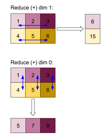
Perhatikan bahwa kedua hasil pengurangan adalah array 1D. Diagram menunjukkan satu kolom sebagai kolom dan satu lagi sebagai baris hanya untuk kemudahan visual.
Untuk contoh yang lebih kompleks, berikut adalah array 3D. Peringkatnya adalah 3, dimensi 0 dari ukuran 4, dimensi 1 dari ukuran 2, dan dimensi 2 dari ukuran 3. Untuk mempermudah, nilai 1 hingga 6 direplikasi di seluruh dimensi 0.
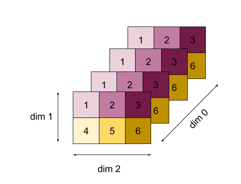
Sama seperti contoh 2D, kita hanya dapat mengurangi satu dimensi. Misalnya, jika kita mengurangi dimensi 0, kita akan mendapatkan array peringkat 2 dengan semua nilai di dimensi 0 dilipat menjadi skalar:
|  4   8  12 |
| 16  20  24 |
Jika kita mengurangi dimensi 2, kita juga mendapatkan array peringkat 2 dengan semua nilai di seluruh dimensi 2 dilipat menjadi skalar:
| 6  15 |
| 6  15 |
| 6  15 |
| 6  15 |
Perhatikan bahwa urutan relatif antara dimensi yang tersisa dalam input dipertahankan dalam output, tetapi beberapa dimensi mungkin akan diberi angka baru (karena peringkat berubah).
Kita juga bisa mengurangi
beberapa dimensi. Menambahkan dimensi 0 dan 1 yang mengurangi
menghasilkan array 1D [20, 28, 36].
Mengurangi array 3D pada semua dimensinya menghasilkan 84 skalar.
Pengurangan Variadik
Saat N > 1, kurangi aplikasi fungsi sedikit lebih kompleks, karena
diterapkan secara bersamaan ke semua input. Operand diberikan ke
komputasi dengan urutan berikut:
- Menjalankan nilai yang dikurangi untuk operand pertama
- ...
- Menjalankan nilai yang dikurangi untuk operand ke-N
- Nilai input untuk operand pertama
- ...
- Nilai input untuk operand ke-N
Misalnya, pertimbangkan fungsi reduksi berikut, yang dapat digunakan untuk menghitung nilai maksimum dan argmax dari array 1-D secara paralel:
f: (Float, Int, Float, Int) -> Float, Int
f(max, argmax, value, index):
  if value >= max:
    return (value, index)
  else:
    return (max, argmax)
Untuk array Input 1-D V = Float[N], K = Int[N], dan nilai init
I_V = Float, I_K = Int, hasil f_(N-1) pengurangan di satu-satunya
dimensi input setara dengan aplikasi rekursif berikut:
f_0 = f(I_V, I_K, V_0, K_0)
f_1 = f(f_0.first, f_0.second, V_1, K_1)
...
f_(N-1) = f(f_(N-2).first, f_(N-2).second, V_(N-1), K_(N-1))
Menerapkan pengurangan ini ke array nilai, dan array indeks berurutan (yaitu iota), akan melakukan iterasi bersama pada array tersebut, dan menampilkan tuple yang berisi nilai maksimal dan indeks yang cocok.
ReducePrecision
Lihat juga
XlaBuilder::ReducePrecision.
Memodelkan efek konversi nilai floating point ke format presisi yang lebih rendah (seperti IEEE-FP16) dan kembali ke format aslinya. Jumlah bit eksponen dan mantissa dalam format presisi lebih rendah dapat ditentukan secara arbitrer, meskipun semua ukuran bit mungkin tidak didukung di semua implementasi hardware.
ReducePrecision(operand, mantissa_bits, exponent_bits)
| Argumen | Jenis | Semantik |
|---|---|---|
operand |
XlaOp |
array jenis floating point T. |
exponent_bits |
int32 |
jumlah bit eksponen dalam format presisi lebih rendah |
mantissa_bits |
int32 |
jumlah bit mantissa dalam format presisi lebih rendah |
Hasilnya adalah array jenis T. Nilai input dibulatkan ke nilai terdekat
yang dapat diwakili dengan jumlah bit mantissa tertentu (menggunakan semantik "ties to merata"), dan nilai apa pun yang melebihi rentang yang ditentukan oleh jumlah
bit eksponen akan dibulatkan ke tak terbatas positif atau negatif. Nilai NaN
dipertahankan, meskipun dapat dikonversi menjadi nilai NaN kanonis.
Format presisi lebih rendah harus memiliki minimal satu bit eksponen (untuk membedakan nilai nol dari tak terhingga, karena keduanya memiliki mantissa nol), dan harus memiliki jumlah bit mantissa yang tidak negatif. Jumlah bit eksponen atau
mantissa dapat melebihi nilai yang sesuai untuk jenis T; bagian
konversi yang sesuai hanya merupakan tanpa pengoperasian.
ReduceScatter
Lihat juga
XlaBuilder::ReduceScatter.
RedScatter adalah operasi kolektif yang secara efektif melakukan AllReduce, lalu menyebarkan hasilnya dengan membaginya menjadi blok shard_count di sepanjang scatter_dimension dan replika i dalam grup replika yang menerima shard ith.
ReduceScatter(operand, computation, scatter_dim, shard_count,
replica_group_ids, channel_id)
| Argumen | Jenis | Semantik |
|---|---|---|
operand |
XlaOp |
Array atau tuple array yang tidak kosong untuk dikurangi di seluruh replika. |
computation |
XlaComputation |
Komputasi pengurangan |
scatter_dimension |
int64 |
Dimensi yang akan disebar. |
shard_count |
int64 |
Jumlah blok yang akan dibagi scatter_dimension |
replica_groups |
vektor vektor int64 |
Grup di mana pengurangan dilakukan |
channel_id |
int64 opsional |
ID saluran opsional untuk komunikasi lintas modul |
- Jika
operandadalah tuple array, pengurangan sebar akan dijalankan pada setiap elemen tuple. replica_groupsadalah daftar grup replika tempat pengurangan dilakukan (ID replika untuk replika saat ini dapat diambil menggunakanReplicaId). Urutan replika dalam setiap grup menentukan urutan penyebaran hasil semua pengurangan.replica_groupsharus kosong (dalam hal ini semua replika dimiliki satu grup), atau berisi jumlah elemen yang sama dengan jumlah replika. Jika ada lebih dari satu grup replika, semua grup replika tersebut harus berukuran sama. Misalnya,replica_groups = {0, 2}, {1, 3}melakukan pengurangan antara replika0dan2, serta1dan3, lalu menyebarkan hasilnya.shard_countadalah ukuran setiap grup replika. Kita memerlukannya jikareplica_groupskosong. Jikareplica_groupstidak kosong,shard_countharus sama dengan ukuran setiap grup replika.channel_iddigunakan untuk komunikasi lintas modul: hanya operasireduce-scatterdenganchannel_idyang sama yang dapat saling berkomunikasi.
Bentuk output adalah bentuk input dengan scatter_dimension yang dibuat
shard_count kali lebih kecil. Misalnya, jika ada dua replika dan
operand memiliki nilai [1.0, 2.25] dan [3.0, 5.25] masing-masing pada kedua
replika tersebut, nilai output dari operasi ini dengan scatter_dim adalah 0 akan menjadi
[4.0] untuk replika pertama dan [7.5] untuk replika kedua.
ReduceWindow
Lihat juga
XlaBuilder::ReduceWindow.
Menerapkan fungsi reduksi ke semua elemen di setiap jendela dari urutan array multi-dimensi N, yang menghasilkan satu atau tuple array multi-dimensi N sebagai output. Setiap array output memiliki jumlah elemen yang sama dengan
jumlah posisi jendela yang valid. Lapisan penggabungan dapat dinyatakan sebagai
ReduceWindow. Serupa dengan Reduce, computation yang diterapkan
selalu diteruskan init_values di sisi kiri.
ReduceWindow(operands..., init_values..., computation, window_dimensions,
window_strides, padding)
| Argumen | Jenis | Semantik |
|---|---|---|
operands |
N XlaOps |
Urutan array multi-dimensi N dari jenis T_0,..., T_{N-1}, masing-masing mewakili area dasar tempat jendela ditempatkan. |
init_values |
N XlaOps |
Nilai awal N untuk pengurangan, satu untuk setiap operand N. Baca artikel Mengurangi untuk mengetahui detailnya. |
computation |
XlaComputation |
Fungsi pengurangan jenis T_0, ..., T_{N-1}, T_0, ..., T_{N-1} -> Collate(T_0, ..., T_{N-1}), untuk diterapkan ke elemen di setiap jendela dari semua operand input. |
window_dimensions |
ArraySlice<int64> |
array bilangan bulat untuk nilai dimensi jendela |
window_strides |
ArraySlice<int64> |
array bilangan bulat untuk nilai langkah jendela |
base_dilations |
ArraySlice<int64> |
array bilangan bulat untuk nilai dilatasi basis |
window_dilations |
ArraySlice<int64> |
array bilangan bulat untuk nilai dilatasi jendela |
padding |
Padding |
jenis padding untuk jendela (Padding::kSame, yang memberi bantalan agar memiliki bentuk output yang sama dengan input jika langkah adalah 1, atau Padding::kValid, yang tidak menggunakan padding dan "menghentikan" jendela setelah tidak lagi cocok) |
Dengan keterangan:
- N harus lebih besar atau sama dengan 1.
- Semua array input harus memiliki dimensi yang sama.
- Jika
N = 1,Collate(T)adalahT. - Jika
N > 1,Collate(T_0, ..., T_{N-1})adalah tuple dari elemenNdari jenis(T0,...T{N-1}).
Kode dan gambar di bawah menunjukkan contoh penggunaan ReduceWindow. Input adalah
matriks berukuran [4x6], dan window_dimensions dan window_stride_dimensions bernilai
[2x3].
// Create a computation for the reduction (maximum).
XlaComputation max;
{
  XlaBuilder builder(client_, "max");
  auto y = builder.Parameter(0, ShapeUtil::MakeShape(F32, {}), "y");
  auto x = builder.Parameter(1, ShapeUtil::MakeShape(F32, {}), "x");
  builder.Max(y, x);
  max = builder.Build().value();
}

// Create a ReduceWindow computation with the max reduction computation.
XlaBuilder builder(client_, "reduce_window_2x3");
auto shape = ShapeUtil::MakeShape(F32, {4, 6});
auto input = builder.Parameter(0, shape, "input");
builder.ReduceWindow(
    input,
    /*init_val=*/builder.ConstantLiteral(LiteralUtil::MinValue(F32)),
    *max,
    /*window_dimensions=*/{2, 3},
    /*window_stride_dimensions=*/{2, 3},
    Padding::kValid);
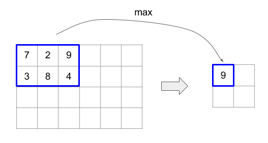
Langkah 1 dalam dimensi menentukan bahwa posisi jendela dalam dimensi berjarak 1 elemen dari jendela yang bersebelahan. Untuk menentukan bahwa tidak ada jendela yang tumpang-tindih satu sama lain, window_stride_dimensions harus sama dengan window_dimensions. Gambar di bawah ini mengilustrasikan penggunaan dua nilai langkah yang berbeda. Padding diterapkan ke setiap dimensi input dan penghitungannya sama seperti meskipun input masuk dengan dimensi yang dimilikinya setelah padding.
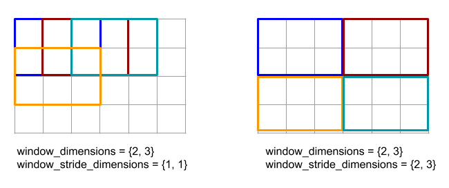
Untuk contoh padding yang tidak umum, pertimbangkan untuk menghitung minimum periode pengurangan
(nilai awal adalah MAX_FLOAT) dengan dimensi 3 dan langkah 2 pada array
input [10000, 1000, 100, 10, 1]. Padding kValid menghitung minimum lebih dari dua
jendela valid: [10000, 1000, 100] dan [100, 10, 1], yang menghasilkan
output [100, 1]. Padding kSame terlebih dahulu menjadi bantalan pada array sehingga bentuk setelah
jendela kurangi akan sama dengan input untuk langkah satu dengan menambahkan elemen
awal di kedua sisi, sehingga mendapatkan [MAX_VALUE, 10000, 1000, 100, 10, 1,
MAX_VALUE]. Menjalankan pengurangan jendela di atas array dengan padding beroperasi di tiga
jendela [MAX_VALUE, 10000, 1000], [1000, 100, 10], [10, 1, MAX_VALUE], dan
menghasilkan [1000, 10, 1].
Urutan evaluasi fungsi pengurangan bersifat arbitrer dan mungkin
non-deterministik. Oleh karena itu, fungsi pengurangan tidak boleh terlalu
sensitif terhadap pengaitan ulang. Lihat diskusi tentang asosiatif dalam
konteks Reduce untuk detail selengkapnya.
ReplicaId
Lihat juga
XlaBuilder::ReplicaId.
Menampilkan ID unik (skalar U32) dari replika.
ReplicaId()
ID unik setiap replika adalah bilangan bulat tanpa tanda tangan dalam interval [0, N), dengan N sebagai jumlah replika. Karena semua replika menjalankan program
yang sama, panggilan ReplicaId() dalam program akan menampilkan nilai yang berbeda pada
setiap replika.
Bentuk ulang
Lihat juga
operasi XlaBuilder::Reshape
dan Collapse.
Membentuk ulang dimensi array menjadi konfigurasi baru.
Reshape(operand, new_sizes)
Reshape(operand, dimensions, new_sizes)
| Argumen | Jenis | Semantik |
|---|---|---|
operand |
XlaOp |
array jenis T |
dimensions |
Vektor int64 |
urutan diciutkan dimensi |
new_sizes |
Vektor int64 |
vektor ukuran dimensi baru |
Secara konseptual, bentuk ulang mula-mula akan meratakan array menjadi vektor nilai data satu dimensi, lalu menyaring vektor ini menjadi bentuk baru. Argumen input
adalah array arbitrer dari jenis T, vektor konstanta waktu kompilasi indeks
dimensi, dan vektor konstanta waktu kompilasi ukuran dimensi untuk hasilnya.
Nilai dalam vektor dimension, jika diberikan, harus berupa permutasi dari semua dimensi T; nilai default jika tidak diberikan adalah {0, ..., rank - 1}. Urutan dimensi dalam dimensions adalah dari dimensi bervariasi paling lambat (paling besar) hingga dimensi tercepat (paling kecil) di nest loop yang menciutkan array input menjadi satu dimensi. Vektor new_sizes menentukan ukuran
array output. Nilai pada indeks 0 di new_sizes adalah ukuran dimensi 0, nilai pada indeks 1 adalah ukuran dimensi 1, dan seterusnya. Produk
dimensi new_size harus sama dengan produk dari ukuran dimensi
operand. Saat menyaring array yang diciutkan menjadi array multidimensi yang ditentukan oleh new_sizes, dimensi di new_sizes akan diurutkan dari
variasi paling lambat (paling utama) dan ke variasi tercepat (paling kecil).
Misalnya, biarkan v menjadi array dari 24 elemen:
let v = f32[4x2x3] { { {10, 11, 12}, {15, 16, 17} },
                    { {20, 21, 22}, {25, 26, 27} },
                    { {30, 31, 32}, {35, 36, 37} },
                    { {40, 41, 42}, {45, 46, 47} } };

In-order collapse:
let v012_24 = Reshape(v, {0,1,2}, {24});
then v012_24 == f32[24] {10, 11, 12, 15, 16, 17, 20, 21, 22, 25, 26, 27,
                         30, 31, 32, 35, 36, 37, 40, 41, 42, 45, 46, 47};

let v012_83 = Reshape(v, {0,1,2}, {8,3});
then v012_83 == f32[8x3] { {10, 11, 12}, {15, 16, 17},
                          {20, 21, 22}, {25, 26, 27},
                          {30, 31, 32}, {35, 36, 37},
                          {40, 41, 42}, {45, 46, 47} };

Out-of-order collapse:
let v021_24 = Reshape(v, {1,2,0}, {24});
then v012_24 == f32[24]  {10, 20, 30, 40, 11, 21, 31, 41, 12, 22, 32, 42,
                          15, 25, 35, 45, 16, 26, 36, 46, 17, 27, 37, 47};

let v021_83 = Reshape(v, {1,2,0}, {8,3});
then v021_83 == f32[8x3] { {10, 20, 30}, {40, 11, 21},
                          {31, 41, 12}, {22, 32, 42},
                          {15, 25, 35}, {45, 16, 26},
                          {36, 46, 17}, {27, 37, 47} };


let v021_262 = Reshape(v, {1,2,0}, {2,6,2});
then v021_262 == f32[2x6x2] { { {10, 20}, {30, 40},
                              {11, 21}, {31, 41},
                              {12, 22}, {32, 42} },
                             { {15, 25}, {35, 45},
                              {16, 26}, {36, 46},
                              {17, 27}, {37, 47} } };
Sebagai kasus khusus, pembentukan ulang dapat mengubah array elemen tunggal menjadi skalar dan sebaliknya. Misalnya,
Reshape(f32[1x1] { {5} }, {0,1}, {}) == 5;
Reshape(5, {}, {1,1}) == f32[1x1] { {5} };
Kebalikan (terbalik)
Lihat juga
XlaBuilder::Rev.
Rev(operand, dimensions)
| Argumen | Jenis | Semantik |
|---|---|---|
operand |
XlaOp |
array jenis T |
dimensions |
ArraySlice<int64> |
untuk membalikkan |
Membalik urutan elemen dalam array operand di sepanjang dimensions yang ditentukan, sehingga menghasilkan array output dengan bentuk yang sama. Setiap elemen array operand pada indeks multidimensi disimpan ke dalam array output pada indeks yang ditransformasi. Indeks multidimensi ditransformasikan dengan membalik indeks di setiap dimensi untuk dibalik (yaitu, jika dimensi ukuran N adalah salah satu dimensi yang berbalik, indeks i-nya diubah menjadi N - 1 - i).
Salah satu kegunaan operasi Rev adalah untuk membalikkan array bobot konvolusi di sepanjang dua dimensi jendela selama komputasi gradien dalam jaringan neural.
RngNormal
Lihat juga
XlaBuilder::RngNormal.
Membuat output bentuk tertentu dengan angka acak yang dihasilkan mengikuti \(N(\mu, \sigma)\) distribusi normal. Parameter \(\mu\) , \(\sigma\), dan bentuk output harus memiliki jenis elemen floating point. Selanjutnya, parameter tersebut harus bernilai skalar.
RngNormal(mu, sigma, shape)
| Argumen | Jenis | Semantik |
|---|---|---|
mu |
XlaOp |
Skalar tipe T yang menentukan rata-rata angka yang dihasilkan |
sigma |
XlaOp |
Skalar tipe T yang menentukan simpangan baku dari |
shape |
Shape |
Bentuk output tipe T |
RngUniform
Lihat juga
XlaBuilder::RngUniform.
Membuat output bentuk tertentu dengan angka acak yang dihasilkan dengan mengikuti distribusi seragam selama interval \([a,b)\). Jenis elemen parameter dan output harus berupa jenis boolean, jenis integral, atau jenis floating point, dan jenisnya harus konsisten. Backend CPU dan GPU saat ini hanya mendukung F64, F32, F16, BF16, S64, U64, S32, dan U32. Selain itu, parameter tersebut harus bernilai skalar. Jika \(b <= a\) hasilnya ditentukan oleh implementasi.
RngUniform(a, b, shape)
| Argumen | Jenis | Semantik |
|---|---|---|
a |
XlaOp |
Skalar tipe T yang menentukan batas bawah interval |
b |
XlaOp |
Skalar tipe T yang menentukan batas atas interval |
shape |
Shape |
Bentuk output tipe T |
RngBitGenerator
Menghasilkan output dengan bentuk tertentu yang diisi dengan bit acak seragam menggunakan algoritma yang ditentukan (atau default backend) dan menampilkan status yang diperbarui (dengan bentuk yang sama seperti status awal) dan data acak yang dihasilkan.
Status awal adalah status awal pembuatan angka acak saat ini. Atribut dan bentuk yang diperlukan serta nilai yang valid bergantung pada algoritma yang digunakan.
Outputnya dijamin sebagai fungsi deterministik dari status awal, tetapi tidak dijamin akan bersifat deterministik antara backend dan versi compiler yang berbeda.
RngBitGenerator(algorithm, key, shape)
| Argumen | Jenis | Semantik |
|---|---|---|
algorithm |
RandomAlgorithm |
algoritma PRNG. |
initial_state |
XlaOp |
Status awal untuk algoritma PRNG. |
shape |
Shape |
Bentuk output untuk data yang dihasilkan. |
Nilai yang tersedia untuk algorithm:
rng_default: Algoritma khusus backend dengan persyaratan bentuk khusus backend.rng_three_fry: Algoritma PRNG berbasis penghitung ThreeFry. Bentukinitial_stateadalahu64[2]dengan nilai arbitrer. Salmon et al. SC 2011. Angka acak paralel: semudah 1, 2, 3.rng_philox: Algoritma Philox untuk menghasilkan angka acak secara paralel. Bentukinitial_stateadalahu64[3]dengan nilai arbitrer. Salmon et al. SC 2011. Angka acak paralel: semudah 1, 2, 3.
Sebar
Operasi sebar XLA menghasilkan urutan hasil yang merupakan nilai
array input operands, dengan beberapa irisan (pada indeks yang ditentukan oleh
scatter_indices) yang diperbarui dengan urutan nilai di updates menggunakan
update_computation.
Lihat juga
XlaBuilder::Scatter.
scatter(operands..., scatter_indices, updates..., update_computation,
index_vector_dim, update_window_dims, inserted_window_dims,
scatter_dims_to_operand_dims)
| Argumen | Jenis | Semantik |
|---|---|---|
operands |
Urutan N XlaOp |
Array N dari jenis T_0, ..., T_N yang akan tersebar. |
scatter_indices |
XlaOp |
Array yang berisi indeks awal dari irisan yang harus disebar. |
updates |
Urutan N XlaOp |
Array N dari jenis T_0, ..., T_N. updates[i] berisi nilai yang harus digunakan untuk menyebarkan operands[i]. |
update_computation |
XlaComputation |
Komputasi yang akan digunakan untuk menggabungkan nilai yang ada dalam array input dan update selama sebar. Komputasi ini harus berjenis T_0, ..., T_N, T_0, ..., T_N -> Collate(T_0, ..., T_N). |
index_vector_dim |
int64 |
Dimensi di scatter_indices yang berisi indeks awal. |
update_window_dims |
ArraySlice<int64> |
Kumpulan dimensi dalam bentuk updates yang merupakan dimensi jendela. |
inserted_window_dims |
ArraySlice<int64> |
Kumpulan dimensi jendela yang harus disisipkan ke dalam bentuk updates. |
scatter_dims_to_operand_dims |
ArraySlice<int64> |
Peta dimensi dari indeks sebar ke ruang indeks operand. Array ini ditafsirkan sebagai memetakan i ke scatter_dims_to_operand_dims[i] . Harus one-to-one dan total. |
indices_are_sorted |
bool |
Apakah indeks dijamin akan diurutkan oleh pemanggil. |
Dengan keterangan:
- N harus lebih besar atau sama dengan 1.
operands[0], ...,operands[N-1] harus memiliki dimensi yang sama.updates[0], ...,updates[N-1] harus memiliki dimensi yang sama.- Jika
N = 1,Collate(T)adalahT. - Jika
N > 1,Collate(T_0, ..., T_N)adalah tuple dari elemenNjenisT.
Jika index_vector_dim sama dengan scatter_indices.rank, secara implisit kami menganggap
scatter_indices memiliki dimensi 1 di akhir.
Kami menentukan update_scatter_dims dari jenis ArraySlice<int64> sebagai kumpulan
dimensi dalam bentuk updates yang tidak dalam update_window_dims, dalam urutan
naik.
Argumen scatter harus mengikuti batasan ini:
Setiap array
updatesharus berperingkatupdate_window_dims.size + scatter_indices.rank - 1.Batas dimensi
idi setiap arrayupdatesharus sesuai dengan hal berikut:- Jika
iada diupdate_window_dims(yaitu sama denganupdate_window_dims[k] untuk beberapak), batas dimensiidiupdatestidak boleh melebihi batasoperandyang sesuai setelah menghitunginserted_window_dims(yaituadjusted_window_bounds[k], denganadjusted_window_boundsberisi batasoperanddengan batas pada indeksinserted_window_dimsdihapus). - Jika
iada diupdate_scatter_dims(yaitu sama denganupdate_scatter_dims[k] untuk beberapak), maka batas dimensiidalamupdatesharus sama dengan batasscatter_indicesyang sesuai, melewatiindex_vector_dim(yaituscatter_indices.shape.dims[k], jikak<index_vector_dimdanscatter_indices.shape.dims[k+1] sebaliknya).
- Jika
update_window_dimsharus dalam urutan menaik, tidak memiliki nomor dimensi berulang, dan berada dalam rentang[0, updates.rank).inserted_window_dimsharus dalam urutan menaik, tidak memiliki nomor dimensi berulang, dan berada dalam rentang[0, operand.rank).operand.rankharus sama dengan jumlahupdate_window_dims.sizedaninserted_window_dims.size.scatter_dims_to_operand_dims.sizeharus sama denganscatter_indices.shape.dims[index_vector_dim], dan nilainya harus berada dalam rentang[0, operand.rank).
Untuk indeks tertentu U dalam setiap array updates, indeks I yang terkait dalam array operands terkait tempat update ini diterapkan dihitung sebagai berikut:
- Misalkan
G= {U[k] untukkdalamupdate_scatter_dims}. GunakanGuntuk mencari vektor indeksSdalam arrayscatter_indicessehinggaS[i] =scatter_indices[Gabungkan(G,i)] tempat Gabungkan(A, b) menyisipkan b pada posisiindex_vector_dimke A. - Buat indeks
Sinke dalamoperandmenggunakanSdengan menyebarkanSmenggunakan petascatter_dims_to_operand_dims. Secara lebih formal:Sin[scatter_dims_to_operand_dims[k]] =S[k] jikak<scatter_dims_to_operand_dims.size.Sin[_] =0jika sebaliknya.
- Buat indeks
Winke dalam setiap arrayoperandsdengan menyebarkan indeks padaupdate_window_dimsdiUsesuai denganinserted_window_dims. Secara lebih formal:Win[window_dims_to_operand_dims(k)] =U[k] jikakberada diupdate_window_dims, denganwindow_dims_to_operand_dimsadalah fungsi monotonik dengan domain [0,update_window_dims.size) dan rentang [0,operand.rank) \inserted_window_dims. (Misalnya, jikaupdate_window_dims.sizeadalah4,operand.rankadalah6, daninserted_window_dimsadalah {0,2}, makawindow_dims_to_operand_dimsadalah {0→1,1→3,2→4,3→5}).Win[_] =0jika sebaliknya.
IadalahWin+Sindengan + adalah penambahan menurut elemen.
Singkatnya, operasi pencar dapat didefinisikan sebagai berikut.
- Lakukan inisialisasi
outputdenganoperands, yaitu untuk semua indeksJ, untuk semua indeksOdalam arrayoperands[J]:
output[J][O] =operands[J][O] - Untuk setiap indeks
Udalam arrayupdates[J] dan indeks yang sesuaiOdalam arrayoperand[J], jikaOadalah indeks yang valid untukoutput:
(output[0][O], ...,output[N-1][O]) =update_computation(output[0][O], ..., ,output[N-1][O],updates[0][U], ...,updates[N-1][U])
Urutan penerapan pembaruan bersifat non-deterministik. Jadi, jika beberapa
indeks dalam updates merujuk ke indeks yang sama di operands, nilai
yang sesuai di output akan bersifat non-deterministik.
Perhatikan bahwa parameter pertama yang diteruskan ke update_computation akan
selalu menjadi nilai saat ini dari array output dan parameter kedua
akan selalu menjadi nilai dari array updates. Hal ini penting
khususnya untuk kasus saat update_computation tidak komutatif.
Jika indices_are_sorted disetel ke benar (true), XLA dapat mengasumsikan bahwa start_indices
diurutkan (dalam urutan start_index_map menaik) oleh pengguna. Jika tidak,
semantik akan ditetapkan.
Secara informal, operasi sebar dapat dilihat sebagai kebalikan dari operasi pengumpulan, yaitu operasi sebar mengupdate elemen dalam input yang diekstrak oleh operasi pengumpulan yang sesuai.
Untuk deskripsi dan contoh informal yang mendetail, lihat bagian
"Deskripsi informal" di Gather.
Pilih
Lihat juga
XlaBuilder::Select.
Membuat array output dari elemen dua array input, berdasarkan nilai array predikat.
Select(pred, on_true, on_false)
| Argumen | Jenis | Semantik |
|---|---|---|
pred |
XlaOp |
array jenis PRED |
on_true |
XlaOp |
array jenis T |
on_false |
XlaOp |
array jenis T |
Array on_true dan on_false harus memiliki bentuk yang sama. Ini juga merupakan
bentuk dari {i>output <i}tersebut. Array pred harus memiliki dimensi yang sama dengan
on_true dan on_false, dengan jenis elemen PRED.
Untuk setiap elemen P dari pred, elemen array output yang sesuai
diambil dari on_true jika nilai P adalah true, dan dari on_false jika
nilai P adalah false. Sebagai bentuk penyiaran yang dibatasi,
pred dapat berupa skalar berjenis PRED. Dalam hal ini, array output diambil
sepenuhnya dari on_true jika pred adalah true, dan dari on_false jika pred adalah false.
Contoh dengan pred non-skalar:
let pred: PRED[4] = {true, false, false, true};
let v1: s32[4] = {1, 2, 3, 4};
let v2: s32[4] = {100, 200, 300, 400};
==>
Select(pred, v1, v2) = s32[4]{1, 200, 300, 4};
Contoh dengan skalar pred:
let pred: PRED = true;
let v1: s32[4] = {1, 2, 3, 4};
let v2: s32[4] = {100, 200, 300, 400};
==>
Select(pred, v1, v2) = s32[4]{1, 2, 3, 4};
Mendukung pilihan di antara tuple. Tuple dianggap sebagai jenis skalar untuk tujuan ini. Jika on_true dan on_false adalah tupel (yang harus memiliki
bentuk yang sama!) maka pred harus merupakan skalar berjenis PRED.
SelectAndScatter
Lihat juga
XlaBuilder::SelectAndScatter.
Operasi ini dapat dianggap sebagai operasi komposit yang pertama-tama menghitung
ReduceWindow pada array operand untuk memilih elemen dari setiap jendela, lalu
menyebarkan array source ke indeks elemen yang dipilih untuk
membuat array output dengan bentuk yang sama dengan array operand. Fungsi select biner digunakan untuk memilih elemen dari setiap jendela dengan menerapkannya ke setiap jendela, dan fungsi ini dipanggil dengan properti bahwa vektor indeks parameter pertama secara leksikografis lebih kecil daripada vektor indeks parameter kedua. Fungsi select akan menampilkan true jika parameter pertama
dipilih dan menampilkan false jika parameter kedua dipilih, dan
fungsi harus memiliki transitivitas (yaitu, jika select(a, b) dan select(b, c) adalah
true, maka select(a, c) juga true) sehingga elemen yang dipilih tidak
bergantung pada urutan elemen yang dilintasi untuk jendela tertentu.
Fungsi scatter diterapkan pada setiap indeks yang dipilih dalam array output. Dibutuhkan dua parameter skalar:
- Nilai saat ini pada indeks yang dipilih dalam array output
- Nilai sebar dari
sourceyang berlaku untuk indeks yang dipilih
Fungsi ini menggabungkan dua parameter dan menampilkan nilai skalar yang digunakan untuk memperbarui nilai pada indeks yang dipilih dalam array output. Awalnya, semua indeks array output ditetapkan ke init_value.
Array output memiliki bentuk yang sama dengan array operand dan array source harus memiliki bentuk yang sama dengan hasil penerapan operasi ReduceWindow pada array operand. SelectAndScatter dapat digunakan untuk
menyebarkan mundur nilai gradien untuk lapisan penggabungan di jaringan neural.
SelectAndScatter(operand, select, window_dimensions, window_strides,
padding, source, init_value, scatter)
| Argumen | Jenis | Semantik |
|---|---|---|
operand |
XlaOp |
array jenis T di mana jendela bergeser |
select |
XlaComputation |
komputasi biner jenis T, T -> PRED, untuk diterapkan ke semua elemen di setiap jendela; menampilkan true jika parameter pertama dipilih dan menampilkan false jika parameter kedua dipilih |
window_dimensions |
ArraySlice<int64> |
array bilangan bulat untuk nilai dimensi jendela |
window_strides |
ArraySlice<int64> |
array bilangan bulat untuk nilai langkah jendela |
padding |
Padding |
jenis padding untuk jendela (Padding::kSame atau Padding::kValid) |
source |
XlaOp |
array jenis T dengan nilai yang akan disebar |
init_value |
XlaOp |
nilai skalar jenis T untuk nilai awal array output |
scatter |
XlaComputation |
komputasi biner jenis T, T -> T, untuk menerapkan setiap elemen sumber sebar dengan elemen tujuannya |
Gambar di bawah menunjukkan contoh penggunaan SelectAndScatter, dengan fungsi select yang menghitung nilai maksimal di antara parameternya. Perhatikan bahwa saat
jendela tumpang-tindih, seperti pada gambar (2) di bawah, indeks array operand dapat
dipilih beberapa kali oleh jendela yang berbeda. Pada gambar, elemen
nilai 9 dipilih oleh kedua jendela atas (biru dan merah) dan fungsi scatter penambahan
biner menghasilkan elemen output nilai 8 (2 + 6).
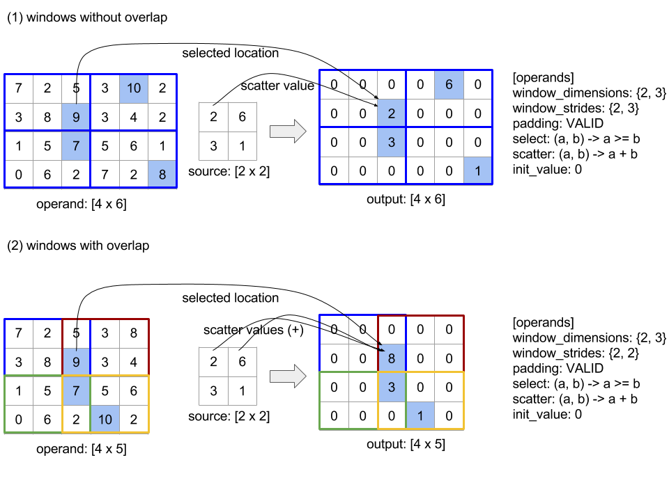
Urutan evaluasi fungsi scatter bersifat arbitrer dan mungkin
non-deterministik. Oleh karena itu, fungsi scatter tidak boleh terlalu
sensitif terhadap pengaitan ulang. Lihat diskusi tentang asosiatif dalam
konteks Reduce untuk detail selengkapnya.
Kirim
Lihat juga
XlaBuilder::Send.
Send(operand, channel_handle)
| Argumen | Jenis | Semantik |
|---|---|---|
operand |
XlaOp |
data yang akan dikirim (array jenis T) |
channel_handle |
ChannelHandle |
ID unik untuk setiap pasangan pengirim/penerima |
Mengirim data operand yang diberikan ke petunjuk Recv dalam komputasi lain
yang memiliki handle saluran yang sama. Tidak menampilkan data apa pun.
Serupa dengan operasi Recv, API klien dari operasi Send mewakili
komunikasi sinkron, dan diurai secara internal menjadi 2 petunjuk HLO
(Send dan SendDone) untuk mengaktifkan transfer data asinkron. Lihat juga
HloInstruction::CreateSend dan HloInstruction::CreateSendDone.
Send(HloInstruction operand, int64 channel_id)
Memulai transfer asinkron operand ke resource yang dialokasikan oleh
petunjuk Recv dengan ID saluran yang sama. Menampilkan konteks, yang digunakan oleh petunjuk SendDone berikut untuk menunggu penyelesaian transfer data. Konteksnya adalah tuple dari {operand (shape), ID permintaan
(U32)}, dan hanya dapat digunakan oleh petunjuk SendDone.
SendDone(HloInstruction context)
Dengan konteks yang dibuat oleh petunjuk Send, tunggu hingga transfer data selesai. Instruksi tidak menampilkan data apa pun.
Penjadwalan petunjuk channel
Urutan eksekusi dari 4 petunjuk tersebut untuk setiap saluran (Recv, RecvDone,
Send, SendDone) adalah sebagai berikut.
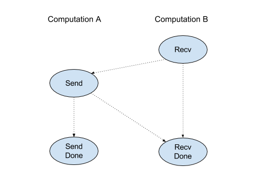
Recvterjadi sebelumSendSendterjadi sebelumRecvDoneRecvterjadi sebelumRecvDoneSendterjadi sebelumSendDone
Saat compiler backend menghasilkan jadwal linear untuk setiap komputasi yang berkomunikasi melalui petunjuk saluran, tidak boleh ada siklus di seluruh komputasi. Misalnya, jadwal di bawah menyebabkan deadlock.
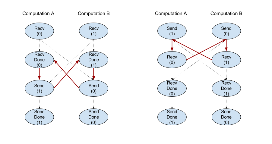
Slice
Lihat juga
XlaBuilder::Slice.
Slice akan mengekstrak sub-array dari array input. Sub-array memiliki peringkat yang sama dengan input dan berisi nilai di dalam kotak pembatas dalam array input tempat dimensi dan indeks kotak pembatas diberikan sebagai argumen untuk operasi slice.
Slice(operand, start_indices, limit_indices, strides)
| Argumen | Jenis | Semantik |
|---|---|---|
operand |
XlaOp |
Array dimensi N jenis T |
start_indices |
ArraySlice<int64> |
Daftar bilangan bulat N yang berisi indeks awal irisan untuk setiap dimensi. Nilai harus lebih besar atau sama dengan nol. |
limit_indices |
ArraySlice<int64> |
Daftar bilangan bulat N yang berisi indeks akhir (eksklusif) untuk irisan setiap dimensi. Setiap nilai harus lebih besar dari atau sama dengan nilai start_indices masing-masing untuk dimensi dan kurang dari atau sama dengan ukuran dimensinya. |
strides |
ArraySlice<int64> |
Daftar bilangan bulat N yang menentukan langkah input dari irisan. Slice ini memilih setiap elemen strides[d] dalam dimensi d. |
Contoh 1 dimensi:
let a = {0.0, 1.0, 2.0, 3.0, 4.0}
Slice(a, {2}, {4}) produces:
  {2.0, 3.0}
Contoh 2 dimensi:
let b =
 { {0.0,  1.0,  2.0},
   {3.0,  4.0,  5.0},
   {6.0,  7.0,  8.0},
   {9.0, 10.0, 11.0} }

Slice(b, {2, 1}, {4, 3}) produces:
  { { 7.0,  8.0},
    {10.0, 11.0} }
Urutkan
Lihat juga
XlaBuilder::Sort.
Sort(operands, comparator, dimension, is_stable)
| Argumen | Jenis | Semantik |
|---|---|---|
operands |
ArraySlice<XlaOp> |
Operand yang akan diurutkan. |
comparator |
XlaComputation |
Komputasi pembanding yang akan digunakan. |
dimension |
int64 |
Dimensi yang akan digunakan untuk mengurutkan. |
is_stable |
bool |
Apakah pengurutan yang stabil akan digunakan. |
Jika hanya satu operand yang disediakan:
Jika operand adalah urutan peringkat 1 (array), hasilnya adalah array yang diurutkan. Jika Anda ingin mengurutkan array dalam urutan menaik, pembanding harus melakukan perbandingan lebih kecil dari. Secara formal, setelah diurutkan, array berlaku untuk semua posisi indeks
i, jdengani < jyang berupacomparator(value[i], value[j]) = comparator(value[j], value[i]) = falseataucomparator(value[i], value[j]) = true.Jika operand memiliki peringkat yang lebih tinggi, operand akan diurutkan di sepanjang dimensi yang diberikan. Misalnya, untuk TensorFlow peringkat 2 (matriks), nilai dimensi
0akan mengurutkan setiap kolom secara independen, dan nilai dimensi1akan mengurutkan setiap baris secara independen. Jika tidak ada nomor dimensi yang diberikan, dimensi terakhir akan dipilih secara default. Untuk dimensi yang diurutkan, urutan penyortiran yang sama berlaku seperti dalam kasus peringkat-1.
Jika operand n > 1 diberikan:
Semua operand
nharus berupa TensorFlow dengan dimensi yang sama. Jenis elemen tensor mungkin berbeda.Semua operand diurutkan bersama, bukan satu per satu. Secara konseptual, operand diperlakukan sebagai tuple. Saat memeriksa apakah elemen setiap operand pada posisi indeks
idanjperlu ditukar, pembanding akan dipanggil dengan parameter skalar2 * n, dengan parameter2 * ksesuai dengan nilai pada posisiidari operandk-th, dan parameter2 * k + 1sesuai dengan nilai pada posisijdari operandk-th. Biasanya, pembanding akan membandingkan parameter2 * kdan2 * k + 1satu sama lain dan mungkin menggunakan pasangan parameter lain sebagai pemutus ikatan.Hasilnya adalah tuple yang terdiri dari operand dalam urutan yang diurutkan (sepanjang dimensi yang diberikan, seperti di atas). Operand
i-thdari tuple sesuai dengan operandi-thdari Sort.
Misalnya, jika ada tiga operand operand0 = [3, 1],
operand1 = [42, 50], operand2 = [-3.0, 1.1], dan pembanding hanya membandingkan
nilai operand0 dengan kurang-dari, maka output pengurutan adalah
tuple ([1, 3], [50, 42], [1.1, -3.0]).
Jika is_stable disetel ke benar (true), pengurutannya dijamin stabil, yaitu, jika
ada elemen yang dianggap sama oleh pembanding, urutan relatif dari nilai yang sama akan dipertahankan. Dua elemen e1 dan e2 sama
jika dan hanya jika comparator(e1, e2) = comparator(e2, e1) = false. Secara default, is_stable ditetapkan ke salah (false).
Transpose
Lihat juga operasi tf.reshape.
Transpose(operand)
| Argumen | Jenis | Semantik |
|---|---|---|
operand |
XlaOp |
Operand yang akan di-transposisi. |
permutation |
ArraySlice<int64> |
Cara membisukan dimensi. |
Membisukan dimensi operand dengan permutasi yang diberikan, sehingga
∀ i . 0 ≤ i < rank ⇒ input_dimensions[permutation[i]] = output_dimensions[i].
Fungsi ini sama dengan Reshape(operand, permutation, Permute(permutation, operand.shape.dimensions)).
TriangularSolve
Lihat juga
XlaBuilder::TriangularSolve.
Menyelesaikan sistem persamaan linear dengan matriks koefisien segitiga bawah atau atas
dengan substitusi maju atau mundur. Menyiarkan bersama dimensi
awal, rutinitas ini menyelesaikan salah satu sistem matriks op(a) * x =
b, atau x * op(a) = b, untuk variabel x, dengan mempertimbangkan a dan b, dengan op(a)
adalah op(a) = a, atau op(a) = Transpose(a), atau op(a) = Conj(Transpose(a)).
TriangularSolve(a, b, left_side, lower, unit_diagonal, transpose_a)
| Argumen | Jenis | Semantik |
|---|---|---|
a |
XlaOp |
array peringkat > 2 dari jenis bilangan kompleks atau floating point dengan bentuk [..., M, M]. |
b |
XlaOp |
array peringkat > 2 dari jenis yang sama dengan bentuk [..., M, K] jika left_side benar, [..., K, M] jika tidak. |
left_side |
bool |
menunjukkan apakah akan menyelesaikan sistem berformat op(a) * x = b (true) atau x * op(a) = b (false). |
lower |
bool |
apakah akan menggunakan segitiga atas atau bawah a. |
unit_diagonal |
bool |
jika true, elemen diagonal a dianggap 1 dan tidak diakses. |
transpose_a |
Transpose |
apakah akan menggunakan a apa adanya, melakukan transposisi, atau mengambil transposisi konjugasinya. |
Data input hanya dibaca dari segitiga bawah/atas a, bergantung pada
nilai lower. Nilai dari segitiga lainnya akan diabaikan. Data output
ditampilkan dalam segitiga yang sama; nilai dalam segitiga lainnya
ditentukan oleh implementasi dan bisa berupa apa saja.
Jika peringkat a dan b lebih besar dari 2, keduanya akan diperlakukan sebagai batch
matriks, dengan semua dimensi kecuali 2 minor adalah dimensi batch. a dan
b harus memiliki dimensi batch yang sama.
Tuple
Lihat juga
XlaBuilder::Tuple.
Tuple yang berisi jumlah variabel handle data, yang masing-masing memiliki bentuknya sendiri.
Ini serupa dengan std::tuple di C++. Secara konseptual:
let v: f32[10] = f32[10]{0, 1, 2, 3, 4, 5, 6, 7, 8, 9};
let s: s32 = 5;
let t: (f32[10], s32) = tuple(v, s);
Tuple dapat didekonstruksi (diakses) melalui operasi GetTupleElement.
Meskipun
Lihat juga
XlaBuilder::While.
While(condition, body, init)
| Argumen | Jenis | Semantik |
|---|---|---|
condition |
XlaComputation |
XlaComputation jenis T -> PRED yang menentukan kondisi penghentian loop. |
body |
XlaComputation |
XlaComputation dari jenis T -> T yang menentukan isi loop. |
init |
T |
Nilai awal untuk parameter condition dan body. |
Secara berurutan mengeksekusi body sampai condition gagal. Hal ini mirip dengan loop sementara dalam banyak bahasa lain, kecuali untuk perbedaan dan batasan yang tercantum di bawah ini.
- Node
Whilemenampilkan nilai jenisT, yang merupakan hasil dari eksekusi terakhirbody. - Bentuk jenis
Tditentukan secara statis dan harus sama di semua iterasi.
Parameter T komputasi diinisialisasi dengan nilai init pada
iterasi pertama dan otomatis diupdate ke hasil baru dari body
di setiap iterasi berikutnya.
Salah satu kasus penggunaan utama node While adalah untuk menerapkan eksekusi berulang
dari pelatihan di jaringan neural. Kode semu yang disederhanakan ditampilkan di bawah ini dengan grafik
yang merepresentasikan komputasi. Kode ini dapat ditemukan di
while_test.cc.
Jenis T dalam contoh ini adalah Tuple yang terdiri dari int32 untuk
jumlah iterasi dan vector[10] untuk akumulator. Untuk 1.000 iterasi, loop terus menambahkan vektor konstan ke akumulator.
// Pseudocode for the computation.
init = {0, zero_vector[10]} // Tuple of int32 and float[10].
result = init;
while (result(0) < 1000) {
  iteration = result(0) + 1;
  new_vector = result(1) + constant_vector[10];
  result = {iteration, new_vector};
}