यहां XlaBuilder इंटरफ़ेस में बताए गए ऑपरेशन के सिमेंटिक्स के बारे में बताया गया है. आम तौर पर, ये कार्रवाइयां xla_data.proto में RPC इंटरफ़ेस में बताई गई कार्रवाइयों से वन-टू-वन मैप करती हैं.
नामकरण के बारे में एक नोट: सामान्य डेटा टाइप XLA में कुछ एक जैसे एलिमेंट (जैसे कि 32-बिट फ़्लोट) मौजूद होते हैं. पूरे दस्तावेज़ में, array का इस्तेमाल आर्बिट्रेरी डाइमेंशन वाले अरे को दिखाने के लिए किया गया है. सुविधा के लिए, खास मामलों में ज़्यादा सटीक और जाने-पहचाने नाम होते हैं. जैसे, वेक्टर 1-डाइमेंशन वाला अरे और मैट्रिक्स 2-डाइमेंशन वाला अरे होता है.
AfterAll
XlaBuilder::AfterAll
भी देखें.
आखिरकार, अलग-अलग संख्या में टोकन लेता है और एक टोकन बनाता है. टोकन शुरुआती टाइप होते हैं. इन्हें ऑर्डर करने के लिए, साइड-इफ़ेक्ट वाली कार्रवाइयों के बीच थ्रेड किया जा सकता है. तय कार्रवाई के बाद, कार्रवाई का ऑर्डर देने के लिए AfterAll को टोकन के तौर पर इस्तेमाल किया जा सकता है.
AfterAll(operands)
| तर्क | टाइप | सिमैंटिक |
|---|---|---|
operands |
XlaOp |
टोकन की अलग-अलग संख्या |
AllGather
XlaBuilder::AllGather
भी देखें.
प्रतिरूपों में स्ट्रिंग जोड़ने की प्रक्रिया करता है.
AllGather(operand, all_gather_dim, shard_count, replica_group_ids,
channel_id)
| तर्क | टाइप | सिमैंटिक |
|---|---|---|
operand
|
XlaOp
|
जवाबों को इकट्ठा करने वाली रेंज |
all_gather_dim |
int64 |
स्ट्रिंग जोड़ने की प्रोसेस का डाइमेंशन |
replica_groups
|
int64 के वेक्टर का वेक्टर |
वे ग्रुप जिनके बीच में स्ट्रिंग जोड़ने की प्रोसेस पूरी की जाती है. |
channel_id
|
वैकल्पिक int64
|
क्रॉस-मॉड्यूल कम्यूनिकेशन के लिए वैकल्पिक चैनल आईडी |
replica_groups, उन रेप्लिका ग्रुप की सूची है जिनके बीच स्ट्रिंग जोड़ने की प्रोसेस की जाती है (मौजूदा कॉपी के लिए रेप्लिका आईडी कोReplicaIdका इस्तेमाल करके फिर से पाया जा सकता है). हर ग्रुप में रेप्लिका के क्रम से यह तय होता है कि नतीजे में उनके इनपुट किस क्रम में दिखेंगे.replica_groupsखाली होना चाहिए (इस स्थिति में सभी प्रतिरूप एक ही समूह से जुड़े होने चाहिए,0सेN - 1तक के क्रम में होने चाहिए) या उनमें उतनी ही संख्या में एलिमेंट होने चाहिए जितनी प्रतिरूपों की संख्या है. उदाहरण के लिए,replica_groups = {0, 2}, {1, 3},0और2के डुप्लीकेट,1और3के बीच स्ट्रिंग जोड़ने की प्रोसेस पूरी करता है.shard_countहर कॉपी ग्रुप का साइज़ होता है. हमें इसकी ज़रूरत तब होती है, जबreplica_groupsखाली हो.channel_idका इस्तेमाल, क्रॉस-मॉड्यूल कम्यूनिकेशन के लिए किया जाता है: एक हीchannel_idवालेall-gatherऑपरेशन ही एक-दूसरे से कम्यूनिकेशन कर सकते हैं.
आउटपुट का आकार, इनपुट का आकार होता है. इसमें all_gather_dim को shard_count गुना बड़ा किया गया है. उदाहरण के लिए, अगर दो रेप्लिका हैं और ऑपरेंड की वैल्यू [1.0, 2.5] और [3.0, 5.25], दोनों कॉपी पर है, तो इस ऑपर्च्यूनिटी की आउटपुट वैल्यू जहां all_gather_dim है, 0 दोनों रेप्लिका पर [1.0, 2.5, 3.0,
5.25] होगा.
AllReduce
XlaBuilder::AllReduce
भी देखें.
प्रतिरूपों में कस्टम गणना करता है.
AllReduce(operand, computation, replica_group_ids, channel_id)
| तर्क | टाइप | सिमैंटिक |
|---|---|---|
operand
|
XlaOp
|
प्रतिरूपों को कम करने के लिए अरे या अरे का टपल |
computation |
XlaComputation |
रिडक्शन कंप्यूटेशन |
replica_groups
|
int64 के वेक्टर का वेक्टर |
वे ग्रुप जिनके बीच में कम की गई कटौती की जाती है. |
channel_id
|
वैकल्पिक int64
|
क्रॉस-मॉड्यूल कम्यूनिकेशन के लिए वैकल्पिक चैनल आईडी |
- जब
operand, ऐरे का एक टपल होता है, तो टपल के हर एलिमेंट पर ऑल-रिड्यूस किया जाता है. replica_groupsउन प्रतिरूप समूहों की सूची है जिनके बीच में कमी की जाती है (मौजूदा प्रतिरूप के लिए रेप्लिका आईडीReplicaIdका इस्तेमाल करके फिर से पाया जा सकता है).replica_groupsखाली होना चाहिए (जिस स्थिति में सभी प्रतिरूप एक ही समूह से जुड़े हों) या उसमें उतनी ही संख्या में एलिमेंट शामिल हों जितने प्रतिरूपों की संख्या में हैं. उदाहरण के लिए,replica_groups = {0, 2}, {1, 3},0और2के साथ-साथ,1और3के डुप्लीकेट कॉपी को प्रोसेस करता है.channel_idका इस्तेमाल, क्रॉस-मॉड्यूल कम्यूनिकेशन के लिए किया जाता है: एक हीchannel_idवालेall-reduceऑपरेशन ही एक-दूसरे से कम्यूनिकेशन कर सकते हैं.
आउटपुट का आकार और इनपुट आकार एक ही होता है. उदाहरण के लिए, अगर दो रेप्लिका हैं और ऑपरेंड की वैल्यू [1.0, 2.5] और [3.0, 5.25] है, तो दोनों कॉपी पर
ऑपरेशन की आउटपुट वैल्यू और समेशन कंप्यूटेशन की वैल्यू [4.0, 7.75] होगी. अगर इनपुट टपल है, तो आउटपुट भी एक टपल है.
AllReduce के नतीजे का हिसाब लगाने के लिए, हर रेप्लिका से एक इनपुट होना ज़रूरी है. इसलिए, अगर कोई एक कॉपी, AllReduce नोड को दूसरे से ज़्यादा बार एक्ज़ीक्यूट करती है, तो पुरानी कॉपी हमेशा इंतज़ार करेगी. सभी प्रतिरूप एक ही प्रोग्राम को चला रहे हैं, इसलिए ऐसा होने के बहुत ज़्यादा तरीके नहीं हैं. हालांकि, ऐसा तब हो सकता है, जब लूप की स्थिति, इनफ़ीड के डेटा पर निर्भर करती है और दिए गए डेटा की वजह से, लूप में होने वाली कार्रवाई किसी अन्य रेप्लिका पर ज़्यादा बार होती है.
AllToAll
XlaBuilder::AllToAll
भी देखें.
AllToAll एक सामूहिक कार्रवाई है, जो सभी कोर से सभी कोर में डेटा भेजती है. इसके दो चरण होते हैं:
- स्कैटर फ़ेज़. हर कोर पर, ऑपरेंड को
split_dimensionsके साथ-साथsplit_countकी संख्या के ब्लॉक में बांटा जाता है और ब्लॉक सभी कोर में बिखर जाते हैं. जैसे, ih ब्लॉक को ith कोर में भेजा जाता है. - इकट्ठा करने का चरण. हर कोर,
concat_dimensionके साथ मिले ब्लॉक को जोड़ता है.
हिस्सा लेने वाले कोर को ऐसे कॉन्फ़िगर किया जा सकता है:
replica_groups: हर ReplicaGroup में कंप्यूटेशन में हिस्सा लेने वाले रेप्लिका आईडी की सूची होती है (मौजूदा कॉपी के लिए रेप्लिका आईडी कोReplicaIdका इस्तेमाल करके फिर से पाया जा सकता है). AllToAll को तय किए गए क्रम में सबग्रुप में लागू किया जाएगा. उदाहरण के लिए,replica_groups = { {1,2,3}, {4,5,0} }का मतलब है कि AllToAll को डुप्लीकेट कॉपी{1, 2, 3}में लागू किया जाएगा और उसे इकट्ठा करने के चरण में, सभी ब्लॉक को 1, 2, 3 के क्रम में ही जोड़ा जाएगा. इसके बाद, एक अन्य AllToAll को रेप्लिका 4, 5, 0 में लागू किया जाएगा और स्ट्रिंग जोड़ने का क्रम भी 4, 5, 0 होगा. अगरreplica_groupsखाली है, तो सभी प्रतिरूप एक ही ग्रुप से जुड़े होते हैं. ऐसा उनके दिखने के क्रम में होता है.
ज़रूरी शर्तें:
split_dimensionपर ऑपरेंड के डाइमेंशन साइज़ कोsplit_countसे भाग दिया जा सकता है.- ऑपरेंड का आकार टपल नहीं होता है.
AllToAll(operand, split_dimension, concat_dimension, split_count,
replica_groups)
| तर्क | टाइप | सिमैंटिक |
|---|---|---|
operand |
XlaOp |
n डाइमेंशन वाले इनपुट ऐरे |
split_dimension
|
int64
|
[0,
n)
इंटरवल में एक वैल्यू, जो उस डाइमेंशन को नाम देती है जिससे ऑपरेंड को स्प्लिट किया जाता है |
concat_dimension
|
int64
|
[0,
n)
में एक वैल्यू, जो उस डाइमेंशन को नाम देती है जिसके साथ स्प्लिट ब्लॉक को जोड़ा जाता है |
split_count
|
int64
|
इस ऑपरेशन में शामिल
कोर की संख्या. अगर replica_groups खाली है, तो यह जवाब की संख्या होनी चाहिए. ऐसा न होने पर, यह हर ग्रुप में मौजूद कॉपी की संख्या के बराबर होनी चाहिए. |
replica_groups
|
ReplicaGroup वेक्टर
|
हर ग्रुप में रेप्लिका आईडी की एक सूची होती है. |
नीचे Alltoall का एक उदाहरण दिया गया है.
XlaBuilder b("alltoall");
auto x = Parameter(&b, 0, ShapeUtil::MakeShape(F32, {4, 16}), "x");
AllToAll(x, /*split_dimension=*/1, /*concat_dimension=*/0, /*split_count=*/4);
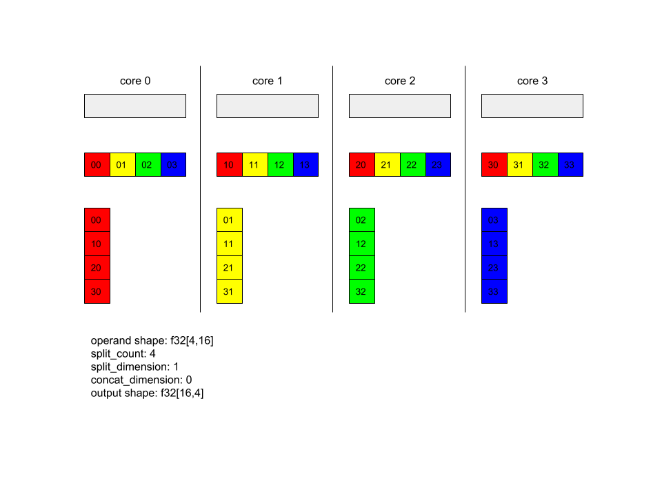
इस उदाहरण में, Alltoall में चार कोर शामिल हैं. हर कोर पर, ऑपरेंड को डाइमेंशन 0 के साथ चार भागों में बांटा जाता है, इसलिए हर हिस्से का आकार f32[4,4] होता है. ये चारों हिस्से सभी कोर में फैले हुए हैं. इसके बाद हर कोर, मिले हुए हिस्सों को डाइमेंशन 1 के साथ कोर 0-4 के क्रम में जोड़ता है. इसलिए, हर कोर के आउटपुट का आकार f32[16,4] होता है.
BatchNormGrad
एल्गोरिदम के बारे में ज़्यादा जानकारी के लिए,
XlaBuilder::BatchNormGrad
और ओरिजनल बैच नॉर्मलाइज़ेशन पेपर
भी देखें.
बैच मानदंड के ग्रेडिएंट की गणना करता है.
BatchNormGrad(operand, scale, mean, variance, grad_output, epsilon, feature_index)
| तर्क | टाइप | सिमैंटिक |
|---|---|---|
operand |
XlaOp |
सामान्य बनाई जाने वाली n डाइमेंशन वाली अरे (x) |
scale |
XlaOp |
1 डाइमेंशन वाला कलेक्शन (\(\gamma\)) |
mean |
XlaOp |
1 डाइमेंशन वाला कलेक्शन (\(\mu\)) |
variance |
XlaOp |
1 डाइमेंशन वाला कलेक्शन (\(\sigma^2\)) |
grad_output |
XlaOp |
BatchNormTraining (\(\nabla y\)) को भेजे गए ग्रेडिएंट |
epsilon |
float |
एप्सिलॉन वैल्यू (\(\epsilon\)) |
feature_index |
int64 |
operand में, सुविधा के डाइमेंशन को इंडेक्स करें |
सुविधा डाइमेंशन की हर सुविधा (operand में सुविधा डाइमेंशन का इंडेक्स feature_index है), के लिए कार्रवाई की जाती है. इसके तहत, बाकी सभी डाइमेंशन के लिए operand, offset, और scale के मुताबिक ग्रेडिएंट की गिनती की जाती है. operand में मौजूद सुविधा डाइमेंशन के लिए, feature_index एक मान्य इंडेक्स होना चाहिए.
तीन ग्रेडिएंट को नीचे दिए गए फ़ॉर्मूला से तय किया जाता है (यह मानते हुए कि
4 डाइमेंशन वाला अरे operand के तौर पर है और जिसमें सुविधा डाइमेंशन इंडेक्स l, बैच साइज़ m, और स्पेशल साइज़ w और h है):
\[ \begin{split} c_l&= \frac{1}{mwh}\sum_{i=1}^m\sum_{j=1}^w\sum_{k=1}^h \left( \nabla y_{ijkl} \frac{x_{ijkl} - \mu_l}{\sigma^2_l+\epsilon} \right) \\\\ d_l&= \frac{1}{mwh}\sum_{i=1}^m\sum_{j=1}^w\sum_{k=1}^h \nabla y_{ijkl} \\\\ \nabla x_{ijkl} &= \frac{\gamma_{l} }{\sqrt{\sigma^2_{l}+\epsilon} } \left( \nabla y_{ijkl} - d_l - c_l (x_{ijkl} - \mu_{l}) \right) \\\\ \nabla \gamma_l &= \sum_{i=1}^m\sum_{j=1}^w\sum_{k=1}^h \left( \nabla y_{ijkl} \frac{x_{ijkl} - \mu_l}{\sqrt{\sigma^2_{l}+\epsilon} } \right) \\\\\ \nabla \beta_l &= \sum_{i=1}^m\sum_{j=1}^w\sum_{k=1}^h \nabla y_{ijkl} \end{split} \]
इनपुट mean और variance बैच और स्पेशल डाइमेंशन में मोमेंट की वैल्यू दिखाते हैं.
आउटपुट टाइप में तीन हैंडल होते हैं:
| आउटपुट | टाइप | सिमैंटिक |
|---|---|---|
grad_operand
|
XlaOp
|
इनपुट operand ($\nabla
x$) के हिसाब से ग्रेडिएंट |
grad_scale
|
XlaOp
|
इनपुट scale ($\nabla
\gamma$) के हिसाब से ग्रेडिएंट |
grad_offset
|
XlaOp
|
इनपुट offset($\nabla
\beta$) के संबंध में ग्रेडिएंट |
BatchNormInference
एल्गोरिदम के बारे में ज़्यादा जानकारी के लिए,
XlaBuilder::BatchNormInference
और ओरिजनल बैच नॉर्मलाइज़ेशन पेपर
भी देखें.
पूरे बैच और स्पेशल डाइमेंशन में किसी अरे को सामान्य बनाता है.
BatchNormInference(operand, scale, offset, mean, variance, epsilon, feature_index)
| तर्क | टाइप | सिमैंटिक |
|---|---|---|
operand |
XlaOp |
सामान्य बनाए जाने के लिए n डाइमेंशन वाला अरे |
scale |
XlaOp |
1 डाइमेंशन वाला अरे |
offset |
XlaOp |
1 डाइमेंशन वाला अरे |
mean |
XlaOp |
1 डाइमेंशन वाला अरे |
variance |
XlaOp |
1 डाइमेंशन वाला अरे |
epsilon |
float |
एप्सिलॉन की वैल्यू |
feature_index |
int64 |
operand में, सुविधा के डाइमेंशन को इंडेक्स करें |
सुविधा डाइमेंशन की हर सुविधा (feature_index, operand में फ़ीचर डाइमेंशन का इंडेक्स है) के लिए, अन्य सभी डाइमेंशन के लिए मीन और वैरियंस कैलकुलेट किया जाता है. साथ ही, operand में हर एलिमेंट को सामान्य बनाने के लिए, मीन और वैरियंस का इस्तेमाल किया जाता है. operand में, सुविधा डाइमेंशन के लिए feature_index एक मान्य इंडेक्स होना चाहिए.
BatchNormInference, हर बैच के लिए mean और variance की गणना किए बिना
BatchNormTraining को कॉल करने के बराबर है. यह अनुमानित वैल्यू के बजाय, mean और
variance इनपुट का इस्तेमाल करता है. इस ऑप का मक़सद,
अनुमान में इंतज़ार का समय कम करना है, इसलिए इसका नाम BatchNormInference है.
आउटपुट एक एन-डाइमेंशन वाला और सामान्य बनाया गया ऐरे है, जिसका आकार इनपुट
operand के जैसा है.
BatchNormTraining
एल्गोरिदम के बारे में ज़्यादा जानकारी के लिए,
XlaBuilder::BatchNormTraining
और the original batch normalization paper
भी देखें.
पूरे बैच और स्पेशल डाइमेंशन में किसी अरे को सामान्य बनाता है.
BatchNormTraining(operand, scale, offset, epsilon, feature_index)
| तर्क | टाइप | सिमैंटिक |
|---|---|---|
operand |
XlaOp |
सामान्य बनाई जाने वाली n डाइमेंशन वाली अरे (x) |
scale |
XlaOp |
1 डाइमेंशन वाला कलेक्शन (\(\gamma\)) |
offset |
XlaOp |
1 डाइमेंशन वाला कलेक्शन (\(\beta\)) |
epsilon |
float |
एप्सिलॉन वैल्यू (\(\epsilon\)) |
feature_index |
int64 |
operand में, सुविधा के डाइमेंशन को इंडेक्स करें |
सुविधा डाइमेंशन की हर सुविधा (feature_index, operand में फ़ीचर डाइमेंशन का इंडेक्स है) के लिए, अन्य सभी डाइमेंशन के लिए मीन और वैरियंस कैलकुलेट किया जाता है. साथ ही, operand में हर एलिमेंट को सामान्य बनाने के लिए, मीन और वैरियंस का इस्तेमाल किया जाता है. operand में, सुविधा डाइमेंशन के लिए feature_index एक मान्य इंडेक्स होना चाहिए.
एल्गोरिदम operand \(x\) के हर बैच के लिए इस तरह काम करता है, जिसमें w और h वाले m एलिमेंट होते हैं. ये एलिमेंट स्पेशल डाइमेंशन के साइज़ के तौर पर होते हैं (यह मानते हुए कि operand
4 डाइमेंशन वाला अरे है):
सुविधा डाइमेंशन में हर सुविधा
lके लिए बैच मीन \(\mu_l\) कैलकुलेट करता है: \(\mu_l=\frac{1}{mwh}\sum_{i=1}^m\sum_{j=1}^w\sum_{k=1}^h x_{ijkl}\)बैच वैरियंस कैलकुलेट करता है \(\sigma^2_l\): $\sigma^2l=\frac{1}{mwh}\sum{i=1}^m\sum{j=1}^w\sum{k=1}^h (x_{ijkl} - \mu_l)^2$
नॉर्मलाइज़, स्केल और शिफ़्ट: \(y_{ijkl}=\frac{\gamma_l(x_{ijkl}-\mu_l)}{\sqrt[2]{\sigma^2_l+\epsilon} }+\beta_l\)
एपिसोड की वैल्यू को ज़ीरो से भाग देने पर दिखने वाली गड़बड़ियों से बचाने के लिए, आम तौर पर एक छोटी संख्या जोड़ी जाती है.
आउटपुट टाइप, तीन XlaOps का टपल है:
| आउटपुट | टाइप | सिमैंटिक |
|---|---|---|
output
|
XlaOp
|
इनपुट के समान आकार वाली n डाइमेंशन वाली अरे
operand (y) |
batch_mean |
XlaOp |
1 डाइमेंशन वाला कलेक्शन (\(\mu\)) |
batch_var |
XlaOp |
1 डाइमेंशन वाला कलेक्शन (\(\sigma^2\)) |
batch_mean और batch_var को ऊपर दिए गए फ़ॉर्मूले का इस्तेमाल करके बैच और स्पेशल डाइमेंशन के
हिसाब से कैलकुलेट किया जाता है.
BitcastConvertType
XlaBuilder::BitcastConvertType
भी देखें.
TensorFlow में दिए गए tf.bitcast की तरह, यह डेटा आकार से टारगेट आकार तक, एलिमेंट के हिसाब से बिटकास्ट कार्रवाई करता है. इनपुट और आउटपुट साइज़ का मेल खाना ज़रूरी है: उदाहरण के लिए, s32 एलिमेंट, बिटकास्ट रूटीन के ज़रिए f32 एलिमेंट बन जाएंगे और एक
s32 एलिमेंट, चार s8 एलिमेंट बन जाएगा. बिटकास्ट को लो-लेवल कास्ट के तौर पर लागू किया जाता है, इसलिए अलग-अलग फ़्लोटिंग-पॉइंट वाली मशीन से अलग-अलग नतीजे मिलेंगे.
BitcastConvertType(operand, new_element_type)
| तर्क | टाइप | सिमैंटिक |
|---|---|---|
operand |
XlaOp |
डिम डी के साथ T टाइप की कैटगरी |
new_element_type |
PrimitiveType |
टाइप U |
ऑपरेंड के डाइमेंशन और टारगेट आकार, आखिरी डाइमेंशन से अलग, एक जैसे होने चाहिए. कन्वर्ज़न के पहले और बाद में, प्रिमिटिव साइज़ के अनुपात से इसमें बदलाव होगा.
सोर्स और डेस्टिनेशन एलिमेंट के टाइप, एक-दूसरे से अलग नहीं होने चाहिए.
बिटकास्ट-बदलाव को अलग-अलग चौड़ाई के प्रिमिटिव टाइप में बदला जा रहा है
BitcastConvert एचएलओ निर्देश उस केस में इस्तेमाल किया जा सकता है जिसमें आउटपुट एलिमेंट टाइप T' का साइज़, इनपुट एलिमेंट T के साइज़ के बराबर न हो. सैद्धांतिक तौर पर, पूरा ऑपरेशन एक बिटकास्ट होता है और उसमें मौजूद बाइट में बदलाव नहीं होता, इसलिए आउटपुट एलिमेंट के आकार को बदलना होगा. B = sizeof(T), B' =
sizeof(T') में ऐसे दो मामले हो सकते हैं.
सबसे पहले, B > B' होने पर, आउटपुट आकार को साइज़ का एक नया माइनर डाइमेंशन मिलता है
B/B'. उदाहरण के लिए:
f16[10,2]{1,0} %output = f16[10,2]{1,0} bitcast-convert(f32[10]{0} %input)
असरदार स्केलर के लिए नियम एक ही रहता है:
f16[2]{0} %output = f16[2]{0} bitcast-convert(f32[] %input)
इसके अलावा, B' > B के लिए निर्देश के लिए इनपुट आकार का आखिरी लॉजिकल डाइमेंशन, B'/B के बराबर होना चाहिए. कन्वर्ज़न के दौरान, यह डाइमेंशन हटा दिया जाता है:
f32[10]{0} %output = f32[10]{0} bitcast-convert(f16[10,2]{1,0} %input)
ध्यान दें कि अलग-अलग बिटचौड़ाई के बीच कन्वर्ज़न, एलिमेंट के हिसाब से नहीं होते.
ब्रॉडकास्ट करना
XlaBuilder::Broadcast
भी देखें.
अरे में डेटा का डुप्लीकेट बनाकर, अरे में डाइमेंशन जोड़ता है.
Broadcast(operand, broadcast_sizes)
| तर्क | टाइप | सिमैंटिक |
|---|---|---|
operand |
XlaOp |
डुप्लीकेट किया जाने वाला अरे |
broadcast_sizes |
ArraySlice<int64> |
नए डाइमेंशन के साइज़ |
नए डाइमेंशन बाईं ओर डाले जाते हैं. इसका मतलब है कि अगर broadcast_sizes में वैल्यू {a0, ..., aN} है और ऑपरेंड के आकार में {b0, ..., bM} डाइमेंशन हैं, तो आउटपुट के आकार में {a0, ..., aN, b0, ..., bM} होंगे.
नए डाइमेंशन, ऑपरेंड की कॉपी में इंडेक्स होते हैं, जैसे कि
output[i0, ..., iN, j0, ..., jM] = operand[j0, ..., jM]
उदाहरण के लिए, अगर operand, 2.0f का एक अदिश f32 है और broadcast_sizes का मान {2, 3} है, तो नतीजा एक श्रेणी होगा जिसमें f32[2, 3] आकार होगा. साथ ही, नतीजे में मिलने वाली सभी वैल्यू 2.0f होंगी.
BroadcastInDim
XlaBuilder::BroadcastInDim
भी देखें.
यह फ़ंक्शन, अरे में डेटा का डुप्लीकेट बनाकर, अरे के साइज़ और रैंक को बड़ा करता है.
BroadcastInDim(operand, out_dim_size, broadcast_dimensions)
| तर्क | टाइप | सिमैंटिक |
|---|---|---|
operand |
XlaOp |
डुप्लीकेट किया जाने वाला अरे |
out_dim_size |
ArraySlice<int64> |
टारगेट आकार के डाइमेंशन के साइज़ |
broadcast_dimensions |
ArraySlice<int64> |
ऑपरेंड आकार का प्रत्येक आयाम लक्ष्य आकार में कौन-से आयाम से संबंधित है |
यह ब्रॉडकास्ट की तरह ही है, लेकिन इसकी मदद से कहीं भी डाइमेंशन जोड़े जा सकते हैं. साथ ही, पहले साइज़ वाले मौजूदा डाइमेंशन को बड़ा किया जा सकता है.
operand को out_dim_size में बताए गए आकार में ब्रॉडकास्ट किया जाता है.
broadcast_dimensions, operand के डाइमेंशन को टारगेट शेप के डाइमेंशन के साथ मैप करता है. इसका मतलब है कि ऑपरेंड के i डाइमेंशन को आउटपुट शेप के
ब्रॉडकास्ट_डाइमेंशन[i]वें डाइमेंशन से मैप किया जाता है. operand के डाइमेंशन का साइज़ 1 होना चाहिए या उसका साइज़, आउटपुट आकार के डाइमेंशन के बराबर होना चाहिए. बाकी डाइमेंशन में, साइज़ 1
के डाइमेंशन भरे हुए हैं. डिजनरेट-डाइमेंशन ब्रॉडकास्टिंग, इसके बाद आउटपुट वाले आकार तक पहुंचने के लिए, इन डिजनरेट डाइमेंशन के साथ ब्रॉडकास्ट करती है. ब्रॉडकास्ट करने वाले पेज पर, इसके बारे में पूरी जानकारी दी गई है.
कॉल
XlaBuilder::Call
भी देखें.
दिए गए तर्कों के साथ कंप्यूटेशन शुरू करता है.
Call(computation, args...)
| तर्क | टाइप | सिमैंटिक |
|---|---|---|
computation |
XlaComputation |
आर्बिट्रेरी टाइप के N पैरामीटर के साथ, T_0, T_1, ..., T_{N-1} -> S टाइप का कैलकुलेशन |
args |
N XlaOp सेकंड का क्रम |
आर्बिट्रेरी टाइप के N आर्ग्युमेंट |
args की एरिटी और टाइप,
computation के पैरामीटर से मेल खाने चाहिए. इसमें कोई args नहीं हो सकता.
कोलेस्की
XlaBuilder::Cholesky
भी देखें.
सिमेट्रिक (हर्मिटियन) पॉज़िटिव निश्चित मैट्रिक्स के बैच के कोलेस्की डिकम्पोज़िशन की गणना करता है.
Cholesky(a, lower)
| तर्क | टाइप | सिमैंटिक |
|---|---|---|
a |
XlaOp |
कोई रैंक > कॉम्प्लेक्स या फ़्लोटिंग-पॉइंट टाइप का 2 अरे. |
lower |
bool |
a के ऊपरी या निचले त्रिभुज का उपयोग करना है या नहीं. |
अगर lower true है, तो निचली-त्रिकोणीय आव्यूहों l की गणना करता है, जैसे कि $a = l .
l^T$. अगर lower false है, तो ऊपरी-त्रिकोणीय मैट्रिक्स u की गणना इस तरह करता है
\(a = u^T . u\).
इनपुट डेटा को सिर्फ़ a के निचले/ऊपरी त्रिकोण से पढ़ा जाता है. हालांकि, यह lower की वैल्यू पर निर्भर करता है. दूसरे त्रिकोण के वैल्यू को नज़रअंदाज़ किया जाता है. आउटपुट डेटा
उसी त्रिभुज में दिखाया जाता है; दूसरे त्रिभुज में दी गई वैल्यू,
लागू करने से तय होती हैं और कुछ भी हो सकती हैं.
अगर a की रैंक 2 से ज़्यादा होती है, तो a को मैट्रिक्स का बैच माना जाता है.
इसमें मामूली दो डाइमेंशन को छोड़कर बाकी सभी डाइमेंशन को बैच डाइमेंशन माना जाता है.
अगर a, सिमेट्रिक (हर्मिटियन) पॉज़िटिव नहीं है, तो नतीजा लागू करने के तरीके के बारे में बताया जाता है.
क्लैंप
XlaBuilder::Clamp
भी देखें.
किसी ऑपरेंड को कम से कम और ज़्यादा से ज़्यादा वैल्यू के बीच की रेंज में जोड़ता है.
Clamp(min, operand, max)
| तर्क | टाइप | सिमैंटिक |
|---|---|---|
min |
XlaOp |
T टाइप की कैटगरी |
operand |
XlaOp |
T टाइप की कैटगरी |
max |
XlaOp |
T टाइप की कैटगरी |
ऑपरेंड और सबसे कम और ज़्यादा से ज़्यादा वैल्यू दिए जाने पर, ऑपरेंड को कम से कम और ज़्यादा से ज़्यादा के बीच की रेंज में लौटाता है, नहीं तो, अगर ऑपरेंड इस सीमा से कम है, तो सबसे कम वैल्यू दिखाता है. अगर ऑपरेंड इस सीमा से ज़्यादा है, तो ज़्यादा से ज़्यादा वैल्यू दिखाता है. इसका मतलब है, clamp(a, x, b) = min(max(a, x), b).
तीनों अरे एक ही आकार के होने चाहिए. इसके अलावा, ब्रॉडकास्ट करना के प्रतिबंधित तरीके के तौर पर, min और/या max, T टाइप के स्केलर हो सकते हैं.
min और max स्केलर के साथ उदाहरण:
let operand: s32[3] = {-1, 5, 9};
let min: s32 = 0;
let max: s32 = 6;
==>
Clamp(min, operand, max) = s32[3]{0, 5, 6};
छोटा करें
XlaBuilder::Collapse और tf.reshape कार्रवाई भी देखें.
किसी अरे के डाइमेंशन को छोटा करके, एक डाइमेंशन बनाता है.
Collapse(operand, dimensions)
| तर्क | टाइप | सिमैंटिक |
|---|---|---|
operand |
XlaOp |
T टाइप की कैटगरी |
dimensions |
int64 वेक्टर |
क्रम में, T के डाइमेंशन का लगातार सबसेट. |
'छोटा करें' विकल्प, ऑपरेंड के डाइमेंशन के दिए गए सबसेट को सिर्फ़ एक डाइमेंशन से बदल देता है. इनपुट आर्ग्युमेंट, T टाइप का आर्बिट्रेरी अरे और डाइमेंशन इंडेक्स के कंपाइल-टाइम-कॉन्सटेंट वेक्टर हैं. डाइमेंशन इंडेक्स, क्रम में (कम से ज़्यादा डाइमेंशन की संख्या) होने चाहिए और T के डाइमेंशन का लगातार सबसेट होना चाहिए. इसलिए, {0, 1, 2}, {0, 1} या {1, 2} सभी मान्य डाइमेंशन सेट हैं, लेकिन
{1, 0} या {0, 2} नहीं हैं. उन्हें एक नए डाइमेंशन से बदल दिया जाता है. उन्हें डाइमेंशन के क्रम में उसी जगह पर रखा जाता है जिस जगह पर उन्हें बदला जाता है. साथ ही, नया डाइमेंशन साइज़, ओरिजनल डाइमेंशन साइज़ के प्रॉडक्ट के बराबर होता है. dimensions में सबसे कम डाइमेंशन की संख्या, लूप नेस्ट में सबसे धीमी डाइमेंशन (सबसे बड़ी) होती है, जो इन डाइमेंशन को छोटा कर देती है. सबसे ज़्यादा डाइमेंशन की संख्या, सबसे तेज़ी से अलग-अलग होती है (सबसे छोटी). अगर आइटम को छोटा करने के सामान्य तरीके की ज़रूरत है, तो tf.reshape ऑपरेटर देखें.
उदाहरण के लिए, v को 24 एलिमेंट की कैटगरी बनाएं:
let v = f32[4x2x3] { { {10, 11, 12},  {15, 16, 17} },
{ {20, 21, 22},  {25, 26, 27} },
{ {30, 31, 32},  {35, 36, 37} },
{ {40, 41, 42},  {45, 46, 47} } };

// Collapse to a single dimension, leaving one dimension.
let v012 = Collapse(v, {0,1,2});
then v012 == f32[24] {10, 11, 12, 15, 16, 17,
20, 21, 22, 25, 26, 27,
30, 31, 32, 35, 36, 37,
40, 41, 42, 45, 46, 47};

// Collapse the two lower dimensions, leaving two dimensions.
let v01 = Collapse(v, {0,1});
then v01 == f32[4x6] { {10, 11, 12, 15, 16, 17},
{20, 21, 22, 25, 26, 27},
{30, 31, 32, 35, 36, 37},
{40, 41, 42, 45, 46, 47} };

// Collapse the two higher dimensions, leaving two dimensions.
let v12 = Collapse(v, {1,2});
then v12 == f32[8x3] { {10, 11, 12},
{15, 16, 17},
{20, 21, 22},
{25, 26, 27},
{30, 31, 32},
{35, 36, 37},
{40, 41, 42},
{45, 46, 47} };
CollectivePermute
XlaBuilder::CollectivePermute
भी देखें.
एक साथ मिलकर डेटा इकट्ठा करने की सुविधा को क्रॉस-रेप्लीक के ज़रिए भेजा और पाया जाता है.
CollectivePermute(operand, source_target_pairs)
| तर्क | टाइप | सिमैंटिक |
|---|---|---|
operand |
XlaOp |
n डाइमेंशन वाले इनपुट ऐरे |
source_target_pairs |
<int64, int64> वेक्टर |
(source_replica_id, target_replica_id) पेयर की सूची. हर जोड़े के लिए, ऑपरेंड को सोर्स रेप्लिका से टारगेट रेप्लिका के लिए भेजा जाता है. |
ध्यान दें कि source_target_pair पर ये पाबंदियां हैं:
- किसी भी दो जोड़ों के लिए एक ही टारगेट रेप्लिका आईडी नहीं होना चाहिए. साथ ही, उनका सोर्स रेप्लिका आईडी एक ही नहीं होना चाहिए.
- अगर प्रतिरूप आईडी किसी भी जोड़े में लक्ष्य नहीं है, तो उस प्रतिरूप पर आउटपुट एक टेंसर है जिसमें इनपुट के आकार के बराबर 0(0) हैं.
जोड़ें
XlaBuilder::ConcatInDim
भी देखें.
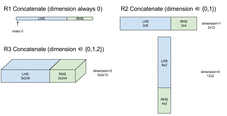
स्ट्रिंग जोड़ने की सुविधा से, कई अरे ऑपरेंड से एक अरे बन जाता है. अरे की रैंक, हर इनपुट ऐरे ऑपरेंड की रैंक के बराबर होती है और उनकी रैंक हर दूसरे ऑपरेंड के बराबर होनी चाहिए. साथ ही, इसमें आर्ग्युमेंट उनके बताए गए क्रम में होते हैं.
Concatenate(operands..., dimension)
| तर्क | टाइप | सिमैंटिक |
|---|---|---|
operands |
N XlaOp का क्रम |
डाइमेंशन [L0, L1, ...] के साथ T टाइप की N कैटगरी. N >= 1 ज़रूरी है. |
dimension |
int64 |
[0, N) इंटरवल में एक वैल्यू, जो operands के बीच जोड़े जाने वाले डाइमेंशन को नाम देती है. |
dimension को छोड़कर, सभी डाइमेंशन एक जैसे होने चाहिए. इसकी वजह यह है कि
XLA, "रैग्ड" कलेक्शन के साथ काम नहीं करता है. यह भी ध्यान दें कि रैंक-0 वैल्यू को जोड़ा नहीं जा सकता (क्योंकि स्ट्रिंग जोड़ने की प्रोसेस वाले डाइमेंशन को नाम देना मुमकिन नहीं है).
1-डाइमेंशन का उदाहरण:
Concat({ {2, 3}, {4, 5}, {6, 7} }, 0)
>>> {2, 3, 4, 5, 6, 7}
दो डाइमेंशन वाला उदाहरण:
let a = {
{1, 2},
{3, 4},
{5, 6},
};
let b = {
{7, 8},
};
Concat({a, b}, 0)
>>> {
{1, 2},
{3, 4},
{5, 6},
{7, 8},
}
डायग्राम:
कंडीशनल
XlaBuilder::Conditional
भी देखें.
Conditional(pred, true_operand, true_computation, false_operand,
false_computation)
| तर्क | टाइप | सिमैंटिक |
|---|---|---|
pred |
XlaOp |
PRED का स्केलर |
true_operand |
XlaOp |
आर्ग्युमेंट टाइप \(T_0\) |
true_computation |
XlaComputation |
XlaComputeation ऑफ़ टाइप \(T_0 \to S\) |
false_operand |
XlaOp |
आर्ग्युमेंट टाइप \(T_1\) |
false_computation |
XlaComputation |
XlaComputeation ऑफ़ टाइप \(T_1 \to S\) |
अगर pred, true है, तो true_computation को प्रोसेस करता है. अगर pred false है, तो false_computation को प्रोसेस करता है और नतीजा दिखाता है.
true_computation को एक ही तरह के आर्ग्युमेंट \(T_0\) में लिया जाना चाहिए. साथ ही, इसे true_operand के साथ शुरू किया जाएगा, जो एक ही तरह का होना चाहिए. false_computation को एक ही तरह के आर्ग्युमेंट \(T_1\) में शामिल किया जाना चाहिए. साथ ही, इसे false_operand के साथ शुरू किया जाएगा, जो एक ही तरह का होना चाहिए. true_computation और false_computation की रिटर्न की गई वैल्यू एक जैसी होनी चाहिए.
ध्यान दें कि pred की वैल्यू के आधार पर true_computation और false_computation में से सिर्फ़ एक को लागू किया जाएगा.
Conditional(branch_index, branch_computations, branch_operands)
| तर्क | टाइप | सिमैंटिक |
|---|---|---|
branch_index |
XlaOp |
S32 का स्केलर |
branch_computations |
N XlaComputation का क्रम |
XlaComputations टाइप की \(T_0 \to S , T_1 \to S , ..., T_{N-1} \to S\) |
branch_operands |
N XlaOp का क्रम |
आर्ग्युमेंट टाइप \(T_0 , T_1 , ..., T_{N-1}\) |
branch_computations[branch_index] को एक्ज़ीक्यूट करता है और नतीजा दिखाता है. अगर
branch_index एक S32 है, जो < 0 या >= N है, तो branch_computations[N-1]
को डिफ़ॉल्ट ब्रांच के तौर पर लागू किया जाता है.
हर branch_computations[b] में एक तरह का आर्ग्युमेंट \(T_b\) होना चाहिए. साथ ही, हर branch_computations[b] को branch_operands[b] के साथ शुरू किया जाएगा, जो एक ही तरह का होना चाहिए. हर branch_computations[b] की रिटर्न की गई वैल्यू एक ही होनी चाहिए.
ध्यान दें कि branch_index की वैल्यू के आधार पर, branch_computations में से सिर्फ़ एक को ही एक्ज़ीक्यूट किया जाएगा.
कन्वर्ज़न (कॉन्वॉल्यूशन)
XlaBuilder::Conv
भी देखें.
ConvWithGeneralPपैडिंग के तौर पर इस्तेमाल किया जा सकता है, लेकिन पैडिंग (जगह) को छोटे तरीके से 'SAME' या 'मान्य' के तौर पर बताया जाता है. SAME पैडिंग, इनपुट (lhs) को शून्य से पैड करती है. इससे वैल्यू को खाते में शामिल न करते समय, इनपुट का आकार इनपुट जैसा ही होता है. मान्य पैडिंग का मतलब है, कोई पैडिंग नहीं.
ConvWithGeneralPadding (कॉन्वॉल्यूशन)
XlaBuilder::ConvWithGeneralPadding
भी देखें.
न्यूरल नेटवर्क में इस्तेमाल किए गए प्रकार के कॉन्वलूशन की गणना करता है. यहां कॉन्वलूशन को एक एन-डाइमेंशन विंडो के तौर पर देखा जा सकता है, जो एन-डाइमेंशन बेस एरिया में चलती है. साथ ही, विंडो की हर संभावित पोज़िशन के लिए कंप्यूटेशन किया जाता है.
| तर्क | टाइप | सिमैंटिक |
|---|---|---|
lhs |
XlaOp |
इनपुट की n+2 ऐरे को रैंक करें |
rhs |
XlaOp |
कर्नेल वेट की n+2 ऐरे को रैंक करें |
window_strides |
ArraySlice<int64> |
कर्नेल स्ट्राइड का n-d अरे |
padding |
ArraySlice< pair<int64,int64>> |
(कम, ज़्यादा) पैडिंग की n-d अरे |
lhs_dilation |
ArraySlice<int64> |
n-d HHs डायलेशन फ़ैक्टर अरे |
rhs_dilation |
ArraySlice<int64> |
n-d rhs फैलाव कारक अरे |
feature_group_count |
int64 | सुविधा ग्रुप की संख्या |
batch_group_count |
int64 | बैच ग्रुप की संख्या |
मान लें कि n स्पेशल डाइमेंशन की संख्या है. lhs आर्ग्युमेंट, रैंक n+2 है, जो बेस एरिया की जानकारी देता है. इसे इनपुट कहा जाता है, हालांकि
बेशक rhs भी एक इनपुट है. न्यूरल नेटवर्क में, ये इनपुट ऐक्टिवेशन होते हैं.
n+2 डाइमेंशन इस क्रम में होते हैं:
batch: इस डाइमेंशन में हर कोऑर्डिनेट एक ऐसे स्वतंत्र इनपुट को दिखाता है जिसके लिए कन्वर्ज़न किया जाता है.z/depth/features: बेस एरिया में हर (y,x) पोज़िशन से एक वेक्टर जुड़ा होता है, जो इस डाइमेंशन में जाता है.spatial_dims:nके उन स्पेशल डाइमेंशन के बारे में बताता है जो उस बेस एरिया को तय करते हैं जहां विंडो चलती है.
rhs आर्ग्युमेंट, रैंक n+2 का ऐरे होता है, जो कॉन्वलूशनल फ़िल्टर/kernel/window में होता है. डाइमेंशन इस क्रम में होते हैं:
output-z: आउटपुट काzडाइमेंशन.input-z: इस डाइमेंशन का साइज़feature_group_count, लाखों मेंzडाइमेंशन के साइज़ के बराबर होना चाहिए.spatial_dims:nके स्पेशल डाइमेंशन के बारे में बताता है. ये डाइमेंशन उस एन-डी विंडो को तय करते हैं जो पूरे बेस एरिया में होती है.
window_strides आर्ग्युमेंट, स्पेशल डाइमेंशन में, कॉन्वलूशनल विंडो के स्ट्रेट के बारे में बताता है. उदाहरण के लिए, अगर पहले आकाशीय डाइमेंशन में स्ट्राइड 3 है, तो विंडो को सिर्फ़ उन निर्देशांकों पर रखा जा सकता है जहां पहले स्पेशल इंडेक्स को तीन से भाग दिया जा सकता है.
padding आर्ग्युमेंट, बेस एरिया पर लागू होने वाली शून्य पैडिंग की संख्या बताता है. पैडिंग (जगह) की संख्या नेगेटिव हो सकती है -- नेगेटिव पैडिंग की कुल वैल्यू, कॉन्वलूशन करने से पहले तय किए गए डाइमेंशन से हटाए जाने वाले एलिमेंट की संख्या दिखाती है. padding[0], y डाइमेंशन के लिए पैडिंग (जगह) तय करता है और padding[1], डाइमेंशन x के लिए पैडिंग (जगह) तय करता है. हर
पेयर में, पहले एलिमेंट के तौर पर कम पैडिंग और दूसरे एलिमेंट के तौर पर ज़्यादा पैडिंग होती है. लो पैडिंग (जगह) को निचले इंडेक्स की दिशा में लागू किया जाता है, जबकि
ज़्यादा पैडिंग (जगह) को ऊपर वाले इंडेक्स की दिशा में लागू किया जाता है. उदाहरण के लिए, अगर
padding[1], (2,3) है, तो बाईं ओर दो शून्य और दूसरे स्पेशल डाइमेंशन में दाईं ओर तीन शून्य होंगे. पैडिंग (जगह) का इस्तेमाल करना, कॉन्वलूशन शुरू करने से पहले इनपुट (lhs) में शून्य वैल्यू को डालने के बराबर होता है.
lhs_dilation और rhs_dilation तर्क, हर जगह के हिसाब से डाइमेंशन में क्रम से लागू होने वाला डाइलेशन फ़ैक्टर तय करते हैं. अगर किसी स्थानिक डाइमेंशन में फैलाव कारक d है, तो उस डाइमेंशन की हर एंट्री के बीच में d-1 छेद लगाए जाते हैं. इससे ऐरे का साइज़ बढ़ जाता है. इन छेदों में बिना किसी वैल्यू के भरे होते हैं, जिसका मतलब है कॉन्वलूशन के लिए ज़ीरो.
आरएच के डायलेशन को एट्रस कन्वलूशन भी कहा जाता है. ज़्यादा जानकारी के लिए, tf.nn.atrous_conv2d देखें. एलएच के डाइल्यूशन को ट्रांसपोज़्ड कॉन्वोलूशन भी कहा जाता है. ज़्यादा जानकारी के लिए, tf.nn.conv2d_transpose देखें.
feature_group_count तर्क (डिफ़ॉल्ट वैल्यू 1) का इस्तेमाल, ग्रुप किए गए कन्वर्ज़न के लिए किया जा सकता है. feature_group_count, इनपुट और आउटपुट सुविधा डाइमेंशन, दोनों का डिवाइज़र होना चाहिए. अगर feature_group_count, 1 से ज़्यादा है, तो इसका मतलब है कि इनपुट और आउटपुट सुविधा के डाइमेंशन और rhsआउटपुट सुविधा को कई feature_group_count ग्रुप में बराबर बांट दिया गया है. हर ग्रुप में, सुविधाओं का क्रम में आने वाला एक से ज़्यादा ग्रुप शामिल है. rhs की इनपुट सुविधा का डाइमेंशन, feature_group_count से भाग दिए गए lhs इनपुट सुविधा के डाइमेंशन के बराबर होना चाहिए, ताकि इनपुट सुविधाओं के ग्रुप का साइज़ पहले से ही मौजूद हो. i-वें ग्रुप का एक साथ इस्तेमाल करके, कई अलग-अलग कन्वलूशन के लिए
feature_group_count का हिसाब लगाया जाता है. इन कन्वर्ज़न के नतीजों को आउटपुट सुविधा डाइमेंशन में एक साथ जोड़ा जाता है.
ज़्यादा बारीकी से कन्वलूशन के लिए, feature_group_count आर्ग्युमेंट को इनपुट सुविधा के डाइमेंशन पर सेट किया जाएगा. साथ ही, फ़िल्टर को
[filter_height, filter_width, in_channels, channel_multiplier] से
[filter_height, filter_width, 1, in_channels * channel_multiplier] में बदल दिया जाएगा. ज़्यादा जानकारी के लिए, tf.nn.depthwise_conv2d देखें.
batch_group_count (डिफ़ॉल्ट वैल्यू 1) आर्ग्युमेंट का इस्तेमाल, बैकप्रोपेगेशन के दौरान, ग्रुप किए गए फ़िल्टर के लिए किया जा सकता है. batch_group_count, lhs (इनपुट) बैच डाइमेंशन के साइज़ का डिवाइज़र होना चाहिए. अगर batch_group_count 1 से बड़ा है, तो इसका मतलब है कि आउटपुट बैच डाइमेंशन का साइज़ input batch
/ batch_group_count होना चाहिए. batch_group_count, आउटपुट सुविधा साइज़ का डिवाइज़र होना चाहिए.
आउटपुट के आकार में ये डाइमेंशन इस क्रम में होते हैं:
batch: इस डाइमेंशन का साइज़batch_group_countलहों मेंbatchडाइमेंशन के साइज़ के बराबर होना चाहिए.z: कर्नेल परoutput-zके बराबर (rhs).spatial_dims: कॉन्वलूशनल विंडो के हर मान्य प्लेसमेंट के लिए एक वैल्यू.

ऊपर दिए गए चित्र से पता चलता है कि batch_group_count फ़ील्ड कैसे काम करता है. असरदार तरीक़े से, हम हर बैच को batch_group_count ग्रुप में बांटते हैं और आउटपुट सुविधाओं के लिए भी ऐसा ही करते हैं. इसके बाद, इनमें से हर ग्रुप के लिए, हम जोड़ी के हिसाब से कन्वलूशन करते हैं और आउटपुट को आउटपुट सुविधा वाले डाइमेंशन के साथ जोड़ते हैं. दूसरे सभी डाइमेंशन (सुविधा और जगह) का ऑपरेशनल सिमैंटिक पहले जैसा ही रहता है.
कॉन्वलूशनल विंडो की मान्य प्लेसमेंट, स्ट्राइड और पैडिंग के बाद बेस एरिया के साइज़ से तय की जाती है.
यह बताने के लिए कि कॉन्वलूशन क्या करता है, 2d कन्वलूशन पर विचार करें और आउटपुट में कुछ तय batch, z, y, x कोऑर्डिनेट चुनें. फिर (y,x), बेस एरिया में विंडो के कोने की पोज़िशन होता है (जैसे, ऊपर बाएं कोने में, इस बात पर निर्भर करता है कि जगह के हिसाब से डाइमेंशन को कैसे समझा जा सकता है). अब हमारे पास बेस एरिया से ली गई एक 2d विंडो है, जहां हर 2d पॉइंट 1d वेक्टर से जुड़ा होता है. इसलिए, हमें 3d बॉक्स मिलता है. कॉन्वलूशनल कर्नेल से, हमने
आउटपुट कोऑर्डिनेट z को ठीक किया है, इसलिए हमारे पास एक 3d बॉक्स भी है. दोनों बॉक्स में एक जैसे
डाइमेंशन होते हैं, इसलिए हम दो बॉक्स के बीच एलिमेंट के हिसाब से प्रॉडक्ट का योग निकाल सकते हैं (डॉट प्रॉडक्ट की तरह). यह आउटपुट वैल्यू है.
ध्यान दें कि अगर output-z 5 है, तो विंडो की हर पोज़िशन, आउटपुट के z डाइमेंशन में
आउटपुट में पांच वैल्यू जनरेट करती है. ये वैल्यू अलग-अलग होती हैं, क्योंकि कॉन्वलूशनल कर्नेल के किस हिस्से का इस्तेमाल किया जाता है - हर output-z कॉर्डिनेट के लिए वैल्यू वाले एक अलग 3d बॉक्स का इस्तेमाल किया जाता है. इसे पांच अलग-अलग कन्वर्ज़न के तौर पर गिना जा सकता है और हर कन्वर्ज़न के लिए अलग फ़िल्टर दिया गया है.
यहां पैडिंग और स्ट्रेडिंग के साथ 2d कॉन्वलूशन के लिए सूडो-कोड दिया गया है:
for (b, oz, oy, ox) {  // output coordinates
  value = 0;
  for (iz, ky, kx) {  // kernel coordinates and input z
    iy = oy*stride_y + ky - pad_low_y;
    ix = ox*stride_x + kx - pad_low_x;
    if ((iy, ix) inside the base area considered without padding) {
      value += input(b, iz, iy, ix) * kernel(oz, iz, ky, kx);
    }
  }
  output(b, oz, oy, ox) = value;
}
ConvertElementType
XlaBuilder::ConvertElementType
भी देखें.
C++ में एलिमेंट के हिसाब से static_cast की तरह, डेटा आकार से टारगेट आकार में एलिमेंट के हिसाब से कन्वर्ज़न कार्रवाई करता है. डाइमेंशन
मैच होने चाहिए और कन्वर्ज़न, एलिमेंट के हिसाब से है. उदाहरण के लिए, s32 एलिमेंट, s32-से-f32 कन्वर्ज़न रूटीन के ज़रिए f32 एलिमेंट बन जाते हैं.
ConvertElementType(operand, new_element_type)
| तर्क | टाइप | सिमैंटिक |
|---|---|---|
operand |
XlaOp |
डिम डी के साथ T टाइप की कैटगरी |
new_element_type |
PrimitiveType |
टाइप U |
ऑपरेंड के डाइमेंशन और टारगेट आकार मैच होने चाहिए. सोर्स और डेस्टिनेशन एलिमेंट टाइप, एक-दूसरे से अलग नहीं होने चाहिए.
T=s32 से U=f32 में होने वाला कन्वर्ज़न, इनट-टू-फ़्लोट कन्वर्ज़न रूटीन करेगा, जैसे कि राउंड-टू-ईवन.
let a: s32[3] = {0, 1, 2};
let b: f32[3] = convert(a, f32);
then b == f32[3]{0.0, 1.0, 2.0}
CrossReplicaSum
योग की गणना करके AllReduce करता है.
CustomCall
XlaBuilder::CustomCall
भी देखें.
कंप्यूटेशन (हिसाब लगाना) में, उपयोगकर्ता के दिए गए फ़ंक्शन को कॉल करें.
CustomCall(target_name, args..., shape)
| तर्क | टाइप | सिमैंटिक |
|---|---|---|
target_name |
string |
फ़ंक्शन का नाम. इस प्रतीक नाम को लक्षित करने वाला एक कॉल निर्देश उत्सर्जित किया जाएगा. |
args |
N XlaOp सेकंड का क्रम |
आर्बिट्रेरी टाइप के N आर्ग्युमेंट, जिन्हें फ़ंक्शन को भेजा जाएगा. |
shape |
Shape |
फ़ंक्शन के आउटपुट का आकार |
arity या आर्ग्युमेंट के टाइप के बावजूद, फ़ंक्शन सिग्नेचर एक जैसा होता है:
extern "C" void target_name(void* out, void** in);
उदाहरण के लिए, अगर CustomCall का इस्तेमाल इस तरह से किया जाता है:
let x = f32[2] {1,2};
let y = f32[2x3] { {10, 20, 30}, {40, 50, 60} };

CustomCall("myfunc", {x, y}, f32[3x3])
यहां myfunc को लागू करने का एक उदाहरण दिया गया है:
extern "C" void myfunc(void* out, void** in) {
  float (&x)[2] = *static_cast<float(*)[2]>(in[0]);
  float (&y)[2][3] = *static_cast<float(*)[2][3]>(in[1]);
  EXPECT_EQ(1, x[0]);
  EXPECT_EQ(2, x[1]);
  EXPECT_EQ(10, y[0][0]);
  EXPECT_EQ(20, y[0][1]);
  EXPECT_EQ(30, y[0][2]);
  EXPECT_EQ(40, y[1][0]);
  EXPECT_EQ(50, y[1][1]);
  EXPECT_EQ(60, y[1][2]);
  float (&z)[3][3] = *static_cast<float(*)[3][3]>(out);
  z[0][0] = x[1] + y[1][0];
  // ...
}
उपयोगकर्ता के दिए गए फ़ंक्शन का इस्तेमाल करने पर कोई खराब असर नहीं होना चाहिए. साथ ही, इसे बिना किसी रुकावट के लागू किया जाना चाहिए.
डॉट
XlaBuilder::Dot
भी देखें.
Dot(lhs, rhs)
| तर्क | टाइप | सिमैंटिक |
|---|---|---|
lhs |
XlaOp |
T टाइप की कैटगरी |
rhs |
XlaOp |
T टाइप की कैटगरी |
इस ऑपरेशन का सटीक सिमेंटिक, ऑपरेंड की रैंक पर निर्भर करता है:
| इनपुट | आउटपुट | सिमैंटिक |
|---|---|---|
वेक्टर [n] dot वेक्टर [n] |
स्केलर | वेक्टर डॉट प्रॉडक्ट |
मैट्रिक्स [m x k] dot वेक्टर [k] |
वेक्टर [m] | मैट्रिक्स-वेक्टर गुणा |
मैट्रिक्स [m x k] dot मैट्रिक्स [k x n] |
मैट्रिक्स [m x n] | मैट्रिक्स-मैट्रिक्स गुणा |
यह कार्रवाई, lhs के दूसरे डाइमेंशन (या
अगर इसकी रैंक 1 है, तो पहले) और rhs के पहले डाइमेंशन के आधार पर, प्रॉडक्ट का योग करती है. ये "कॉन्ट्रैक्टेड" डाइमेंशन होते हैं. lhs और rhs के कॉन्ट्रैक्टेड डाइमेंशन
एक ही साइज़ के होने चाहिए. असल में, इसका इस्तेमाल सदिशों, सदिश/आव्यूहों के गुणन या आव्यूह/आव्यूह के गुणन के बीच
डॉट प्रॉडक्ट लगाने के लिए किया जा सकता है.
DotGeneral
XlaBuilder::DotGeneral
भी देखें.
DotGeneral(lhs, rhs, dimension_numbers)
| तर्क | टाइप | सिमैंटिक |
|---|---|---|
lhs |
XlaOp |
T टाइप की कैटगरी |
rhs |
XlaOp |
T टाइप की कैटगरी |
dimension_numbers |
DotDimensionNumbers |
कॉन्ट्रैक्टिंग और बैच डाइमेंशन नंबर |
यह Dot की तरह है, लेकिन इससे lhs और rhs, दोनों के लिए कॉन्ट्रैक्टिंग और बैच डाइमेंशन नंबर तय किए जा सकते हैं.
| DotडाइमेंशनNumbers फ़ील्ड | टाइप | सिमैंटिक |
|---|---|---|
lhs_contracting_dimensions
|
दोहराया गया int64 | lhs कॉन्ट्रैक्टिंग डाइमेंशन
नंबर |
rhs_contracting_dimensions
|
दोहराया गया int64 | rhs कॉन्ट्रैक्टिंग डाइमेंशन
नंबर |
lhs_batch_dimensions
|
दोहराया गया int64 | lhs बैच डाइमेंशन नंबर |
rhs_batch_dimensions
|
दोहराया गया int64 | rhs बैच डाइमेंशन नंबर |
DotGeneral,
dimension_numbers में बताए गए डाइमेंशन के हिसाब से कुल प्रॉडक्ट का योग करता है.
lhs और rhs से जुड़े कॉन्ट्रैक्टिंग डाइमेंशन नंबर एक जैसे होने ज़रूरी नहीं हैं, लेकिन
उन डाइमेंशन के साइज़ एक जैसे होने चाहिए.
डाइमेंशन नंबर को कॉन्ट्रैक्ट करने का उदाहरण:
lhs = { {1.0, 2.0, 3.0},
{4.0, 5.0, 6.0} }

rhs = { {1.0, 1.0, 1.0},
{2.0, 2.0, 2.0} }

DotDimensionNumbers dnums;
dnums.add_lhs_contracting_dimensions(1);
dnums.add_rhs_contracting_dimensions(1);

DotGeneral(lhs, rhs, dnums) -> { {6.0, 12.0},
{15.0, 30.0} }
lhs और rhs से जुड़े बैच डाइमेंशन नंबर के डाइमेंशन का साइज़ एक जैसा होना चाहिए.
बैच डाइमेंशन नंबर (बैच साइज़ 2, 2x2 मैट्रिक्स) वाला उदाहरण:
lhs = { { {1.0, 2.0},
{3.0, 4.0} },
{ {5.0, 6.0},
{7.0, 8.0} } }

rhs = { { {1.0, 0.0},
{0.0, 1.0} },
{ {1.0, 0.0},
{0.0, 1.0} } }

DotDimensionNumbers dnums;
dnums.add_lhs_contracting_dimensions(2);
dnums.add_rhs_contracting_dimensions(1);
dnums.add_lhs_batch_dimensions(0);
dnums.add_rhs_batch_dimensions(0);

DotGeneral(lhs, rhs, dnums) -> { { {1.0, 2.0},
{3.0, 4.0} },
{ {5.0, 6.0},
{7.0, 8.0} } }
| इनपुट | आउटपुट | सिमैंटिक |
|---|---|---|
[b0, m, k] dot [b0, k, n] |
[b0, मीटर, n] | बैच मैटमुल |
[b0, b1, m, k] dot [b0, b1, k, n] |
[b0, b1, मीटर, n] | बैच मैटमुल |
इसके बाद, मिलता-जुलता डाइमेंशन नंबर बैच डाइमेंशन से शुरू होता है.
इसके बाद, lhs नॉन-कॉन्ट्रैक्टिंग/नॉन-बैच डाइमेंशन और आखिर में rhs
नॉन-कॉन्ट्रैक्टिंग/नॉन-बैच डाइमेंशन से शुरू होता है.
DynamicSlice
XlaBuilder::DynamicSlice
भी देखें.
डाइनैमिकSlice, डाइनैमिक start_indices पर इनपुट ऐरे से कोई सब-ऐरे निकालता है. हर डाइमेंशन में स्लाइस का साइज़ size_indices में पास किया जाता है. इससे हर डाइमेंशन में स्लाइस के खास इंटरवल का आखिरी पॉइंट मिलता है: [start, start + साइज़). start_indices के आकार की रैंक ==
1 होनी चाहिए और डाइमेंशन का साइज़ operand की रैंक के बराबर होना चाहिए.
DynamicSlice(operand, start_indices, size_indices)
| तर्क | टाइप | सिमैंटिक |
|---|---|---|
operand |
XlaOp |
T टाइप की N डाइमेंशन वाली अरे |
start_indices |
N XlaOp का क्रम |
N स्केलर पूर्णांकों की सूची, जिसमें हर डाइमेंशन के स्लाइस के शुरुआती इंडेक्स शामिल हैं. वैल्यू, शून्य से ज़्यादा या उसके बराबर होनी चाहिए. |
size_indices |
ArraySlice<int64> |
N पूर्णांक की सूची, जिसमें हर डाइमेंशन के स्लाइस का साइज़ होता है. हर वैल्यू पूरी तरह से शून्य से ज़्यादा होनी चाहिए. साथ ही, मॉड्यूलो डाइमेंशन साइज़ को रैप होने से बचाने के लिए, शुरुआती + साइज़ डाइमेंशन के साइज़ से कम या उसके बराबर होना चाहिए. |
स्लाइस के असरदार इंडेक्स का हिसाब लगाने के लिए, [1, N) में हर इंडेक्स i के लिए ये ट्रांसफ़ॉर्मेशन ऐक्शन लागू किए जाते हैं. इसके बाद, स्लाइस लागू किए जाते हैं:
start_indices[i] = clamp(start_indices[i], 0, operand.dimension_size[i] - size_indices[i])
इससे यह पक्का होता है कि एक्सट्रैक्ट किया गया स्लाइस, ऑपरेटर और अरे के हिसाब से हमेशा इन-बाउंड है. अगर ट्रांसफ़ॉर्मेशन लागू होने से पहले स्लाइस इन-बाउंड है, तो ट्रांसफ़ॉर्मेशन का कोई असर नहीं होगा.
1-डाइमेंशन का उदाहरण:
let a = {0.0, 1.0, 2.0, 3.0, 4.0}
let s = {2}

DynamicSlice(a, s, {2}) produces:
{2.0, 3.0}
दो डाइमेंशन वाला उदाहरण:
let b =
{ {0.0,  1.0,  2.0},
{3.0,  4.0,  5.0},
{6.0,  7.0,  8.0},
{9.0, 10.0, 11.0} }
let s = {2, 1}

DynamicSlice(b, s, {2, 2}) produces:
{ { 7.0,  8.0},
{10.0, 11.0} }
DynamicUpdateSlice
XlaBuilder::DynamicUpdateSlice
भी देखें.
डाइनैमिकअपडेट स्लाइस, इनपुट ऐरे operand की वैल्यू के तौर पर एक नतीजा जनरेट करता है. इसमें, update स्लाइस को start_indices पर ओवरराइट किया जाता है.
update का आकार, अपडेट किए जाने वाले नतीजे की सब-अरे का आकार तय करता है.
start_indices के आकार की रैंक == 1 होनी चाहिए और डाइमेंशन का साइज़ operand की रैंक के बराबर होना चाहिए.
DynamicUpdateSlice(operand, update, start_indices)
| तर्क | टाइप | सिमैंटिक |
|---|---|---|
operand |
XlaOp |
T टाइप की N डाइमेंशन वाली अरे |
update |
XlaOp |
T टाइप की N डाइमेंशन वाली ऐरे, जिसमें स्लाइस अपडेट है. अपडेट के आकार का हर डाइमेंशन शून्य से ज़्यादा होना चाहिए. साथ ही, अपडेट की शुरुआत और अपडेट, हर डाइमेंशन के ऑपरेंड साइज़ से कम या उसके बराबर होना चाहिए, ताकि आउट-ऑफ़-बाउंड अपडेट इंडेक्स जनरेट न हों. |
start_indices |
N XlaOp का क्रम |
N स्केलर पूर्णांकों की सूची, जिसमें हर डाइमेंशन के स्लाइस के शुरुआती इंडेक्स शामिल हैं. वैल्यू, शून्य से ज़्यादा या उसके बराबर होनी चाहिए. |
स्लाइस के असरदार इंडेक्स का हिसाब लगाने के लिए, [1, N) में हर इंडेक्स i के लिए ये ट्रांसफ़ॉर्मेशन ऐक्शन लागू किए जाते हैं. इसके बाद, स्लाइस लागू किए जाते हैं:
start_indices[i] = clamp(start_indices[i], 0, operand.dimension_size[i] - update.dimension_size[i])
इससे यह पक्का होता है कि अपडेट किया गया स्लाइस, ऑपरेंड अरे के हिसाब से हमेशा इन-बाउंड है. अगर ट्रांसफ़ॉर्मेशन लागू होने से पहले स्लाइस इन-बाउंड है, तो ट्रांसफ़ॉर्मेशन का कोई असर नहीं होगा.
1-डाइमेंशन का उदाहरण:
let a = {0.0, 1.0, 2.0, 3.0, 4.0}
let u = {5.0, 6.0}
let s = {2}

DynamicUpdateSlice(a, u, s) produces:
{0.0, 1.0, 5.0, 6.0, 4.0}
दो डाइमेंशन वाला उदाहरण:
let b =
{ {0.0,  1.0,  2.0},
{3.0,  4.0,  5.0},
{6.0,  7.0,  8.0},
{9.0, 10.0, 11.0} }
let u =
{ {12.0,  13.0},
{14.0,  15.0},
{16.0,  17.0} }

let s = {1, 1}

DynamicUpdateSlice(b, u, s) produces:
{ {0.0,  1.0,  2.0},
{3.0, 12.0, 13.0},
{6.0, 14.0, 15.0},
{9.0, 16.0, 17.0} }
तत्व के अनुसार बाइनरी अंकगणित
XlaBuilder::Add
भी देखें.
इसके लिए, एलिमेंट के हिसाब से बाइनरी अंकगणित की संक्रियाओं का सेट इस्तेमाल किया जा सकता है.
Op(lhs, rhs)
जहां Op, Add (जोड़), Sub (घटाना), Mul
(गुणा), Div (डिविज़न), Rem (बाकी है), Max (ज़्यादा से ज़्यादा), Min
(कम से कम), LogicalAnd (लॉजिकल AND) या LogicalOr (लॉजिकल OR) में से एक है.
| तर्क | टाइप | सिमैंटिक |
|---|---|---|
lhs |
XlaOp |
बाईं ओर का ऑपरेंड: T प्रकार का अरे |
rhs |
XlaOp |
दाईं ओर का ऑपरेंड: T प्रकार का अरे |
आर्ग्युमेंट के आकार एक जैसे या एक जैसे होने चाहिए. ब्रॉडकास्ट करना दस्तावेज़ देखें, ताकि इस बारे में जानकारी मिल सके कि आकार के साथ काम करने का क्या मतलब है. कार्रवाई के नतीजे में एक आकार होता है, जो दो इनपुट ऐरे को ब्रॉडकास्ट करने का नतीजा होता है. इस वैरिएंट में, अलग-अलग रैंक वाली अरे के बीच ऑपरेशन तब तक नहीं किया जाता, जब तक कोई एक ऑपरेंड कोई स्केलर न हो.
जब Op Rem होता है, तो नतीजे का चिह्न भाज्य से लिया जाता है और नतीजे का पूरा मान हमेशा भाजक के निरपेक्ष मान से कम होता है.
इंटीजर डिवीज़न ओवरफ़्लो (शून्य से साइन किया गया/साइन नहीं किया गया डिवीज़न/ज़ीरो से बचा हुआ या -1 के साथ INT_SMIN का साइन किया हुआ डिवीज़न/रिमेंडर) लागू करने से जुड़ी तय वैल्यू जनरेट करता है.
इन ऑपरेशन के लिए, अलग-अलग रैंक वाली ब्रॉडकास्टिंग की सुविधा का एक वैकल्पिक वैरिएंट मौजूद होता है:
Op(lhs, rhs, broadcast_dimensions)
जहां Op, ऊपर दिए गए ईमेल के जैसा है. इस वैरिएंट का इस्तेमाल, अलग-अलग रैंक की रेंज के बीच, अंकगणितीय संक्रियाओं के लिए किया जाना चाहिए. जैसे, वेक्टर में मैट्रिक्स जोड़ना.
अतिरिक्त broadcast_dimensions ऑपरेंड, पूर्णांक का एक हिस्सा होता है. इसका इस्तेमाल, कम रैंक वाले ऑपरेंड की रैंक को
उच्च रैंक वाले ऑपरेंड तक बढ़ाने के लिए किया जाता है. broadcast_dimensions कम रैंक वाले आकार के डाइमेंशन को
ज़्यादा रैंक वाले आकार के डाइमेंशन से मैप करता है. बड़े किए गए आकार के मैप नहीं किए गए डाइमेंशन में,
एक साइज़ के डाइमेंशन भरे हुए होते हैं. डीजन-डाइमेंशन ब्रॉडकास्टिंग
इसके बाद, दोनों ऑपरेंड के आकार को बराबर करने के लिए इन डिजनरेट डाइमेंशन के साथ आकार ब्रॉडकास्ट करता है. ब्रॉडकास्ट करने वाले पेज पर, इनके बारे में पूरी जानकारी दी गई है.
एलिमेंट के हिसाब से तुलना करने की कार्रवाइयां
XlaBuilder::Eq
भी देखें.
स्टैंडर्ड एलिमेंट के मुताबिक बाइनरी की तुलना करने वाली कार्रवाइयों का सेट इस्तेमाल किया जा सकता है. ध्यान दें फ़्लोटिंग-पॉइंट टाइप की तुलना करते समय, स्टैंडर्ड आईईईई 754 फ़्लोट-पॉइंट तुलना सिमैंटिक लागू होते हैं.
Op(lhs, rhs)
जहां Op, Eq (इसके बराबर है), Ne (इसके बराबर नहीं है), Ge
(इससे ज़्यादा या इसके बराबर), Gt (इससे ज़्यादा), Le (इससे कम या इसके बराबर), Lt
(इससे कम) में से कोई एक है. ऑपरेटर के एक और सेट, EqTotalOrder, NeTotalOrder, GeTotalOrder,
GtTotalOrder, LeTotalOrder, और LtTotalOrder. ये सिर्फ़ एक जैसी सुविधाएं उपलब्ध हैं. इनके लिए, -NaN < -Inf < -Finite < -0 < +0 <Nfinite <N
| तर्क | टाइप | सिमैंटिक |
|---|---|---|
lhs |
XlaOp |
बाईं ओर का ऑपरेंड: T प्रकार का अरे |
rhs |
XlaOp |
दाईं ओर का ऑपरेंड: T प्रकार का अरे |
आर्ग्युमेंट के आकार एक जैसे या एक जैसे होने चाहिए. ब्रॉडकास्ट करना दस्तावेज़ देखें, ताकि इस बारे में जानकारी मिल सके कि आकार के साथ काम करने का क्या मतलब है. ऑपरेशन के नतीजे में एक आकार होता है, जो एलिमेंट टाइप PRED के साथ दो इनपुट ऐरे को ब्रॉडकास्ट करने का नतीजा होता है. इस वैरिएंट में, अलग-अलग रैंक वाली अरे के बीच ऑपरेशन तब तक नहीं किया जाता, जब तक कि कोई एक ऑपरेंड कोई स्केलर न हो.
इन ऑपरेशन के लिए, अलग-अलग रैंक वाली ब्रॉडकास्टिंग की सुविधा का एक वैकल्पिक वैरिएंट मौजूद होता है:
Op(lhs, rhs, broadcast_dimensions)
जहां Op, ऊपर दिए गए ईमेल के जैसा है. ऑपरेशन के इस वैरिएंट का इस्तेमाल, अलग-अलग रैंक वाली अरे के बीच ऑपरेशन की तुलना करने के लिए किया जाना चाहिए. जैसे, वेक्टर में मैट्रिक्स जोड़ना.
अतिरिक्त broadcast_dimensions ऑपरेंड, पूर्णांक का एक हिस्सा होता है. इससे ऑपरेंड को ब्रॉडकास्ट करने के लिए इस्तेमाल होने वाले डाइमेंशन के बारे में जानकारी मिलती है. ब्रॉडकास्ट करने वाले पेज पर, इनके बारे में ज़्यादा जानकारी दी गई है.
एलिमेंट के अनुसार यूनरी फ़ंक्शन
XlaBuilder से, एलिमेंट के हिसाब से एक से ज़्यादा फ़ंक्शन इस्तेमाल किए जा सकते हैं:
Abs(operand) एलिमेंट के हिसाब से कुल x -> |x|.
Ceil(operand) एलिमेंट के हिसाब से सेल x -> ⌈x⌉.
Cos(operand) एलिमेंट के हिसाब से कोसाइन x -> cos(x).
Exp(operand) एलिमेंट के हिसाब से नैचुरल एक्स्पोनेंशियल x -> e^x.
Floor(operand) एलिमेंट के हिसाब से फ़्लोर x -> ⌊x⌋.
Imag(operand) एलिमेंट के हिसाब से, कॉम्प्लेक्स (या असली) आकार का काल्पनिक हिस्सा. x -> imag(x). अगर ऑपरेंड फ़्लोटिंग पॉइंट टाइप का है, तो उसकी वैल्यू 0 दिखती है.
IsFinite(operand) यह जांच करता है कि operand का हर एलिमेंट सीमित है या नहीं. जैसे, यह पॉज़िटिव या नेगेटिव अनंतता नहीं है और NaN नहीं है. इनपुट के आकार वाले PRED वैल्यू का अरे दिखाता है. इसमें हर एलिमेंट true होता है, अगर सिर्फ़ संबंधित इनपुट एलिमेंट सीमित हो.
Log(operand) एलिमेंट के हिसाब से नैचुरल लॉगारिद्म x -> ln(x).
LogicalNot(operand) एलिमेंट के हिसाब से लॉजिकल लॉजिकल x -> !(x) नहीं है.
Logistic(operand) एलिमेंट के हिसाब से लॉजिस्टिक फ़ंक्शन का हिसाब x ->
logistic(x).
PopulationCount(operand) operand के हर एलिमेंट में सेट किए गए बिट की संख्या को कैलकुलेट करता है.
Neg(operand) एलिमेंट के हिसाब से निगेशन x -> -x.
Real(operand) जटिल (या असली) आकार का, एलिमेंट के हिसाब से असली हिस्सा.
x -> real(x). अगर ऑपरेंड कोई फ़्लोटिंग पॉइंट टाइप है, तो वही वैल्यू दिखाता है.
Rsqrt(operand) स्क्वेयर रूट कार्रवाई का एलिमेंट के हिसाब से रेसिप्रोकल
x -> 1.0 / sqrt(x).
Sign(operand) एलिमेंट-वाइज़ साइन ऑपरेशन x -> sgn(x) जहां
\[\text{sgn}(x) = \begin{cases} -1 & x < 0\\ -0 & x = -0\\ NaN & x = NaN\\ +0 & x = +0\\ 1 & x > 0 \end{cases}\]
operand के एलिमेंट टाइप की तुलना करने वाले ऑपरेटर का इस्तेमाल करके.
Sqrt(operand) एलिमेंट-वाइज़ स्क्वेयर रूट ऑपरेशन x -> sqrt(x).
Cbrt(operand) एलिमेंट के हिसाब से क्यूबिक रूट की कार्रवाई x -> cbrt(x).
Tanh(operand) एलिमेंट के हिसाब से हाइपरबोलिक टैंजेंट x -> tanh(x).
Round(operand) एलिमेंट के हिसाब से राउंडिंग, शून्य से दूर होता है.
RoundNearestEven(operand) एलिमेंट के हिसाब से राउंडिंग, सबसे नज़दीकी सम संख्या से जुड़ा होता है.
| तर्क | टाइप | सिमैंटिक |
|---|---|---|
operand |
XlaOp |
फ़ंक्शन का ऑपरेंड |
फ़ंक्शन, operand कलेक्शन में मौजूद हर एलिमेंट पर लागू किया जाता है, जिससे एक जैसी आकृति वाली ऐरे बनती है. operand के लिए अदिश (रैंक 0) होने की अनुमति है.
एफ़एफ़टी
XLA FFT कार्रवाई, रीयल और जटिल इनपुट/आउटपुट के लिए फ़ॉरवर्ड और इन्वर्स फूरयर ट्रांसफ़ॉर्म लागू करता है. ज़्यादा से ज़्यादा तीन ऐक्सिस पर मल्टीडाइमेंशन वाले एफ़एफ़टी इस्तेमाल किए जा सकते हैं.
XlaBuilder::Fft
भी देखें.
| तर्क | टाइप | सिमैंटिक |
|---|---|---|
operand |
XlaOp |
हम फूरिये को बदल रहे हैं. |
fft_type |
FftType |
नीचे दी गई टेबल देखें. |
fft_length |
ArraySlice<int64> |
बदली जा रही ऐक्सिस की टाइम-डोमेन लंबाई. यह खास तौर पर IRFFT के लिए सबसे अंदरूनी ऐक्सिस को सही साइज़ देने के लिए ज़रूरी है, क्योंकि RFFT(fft_length=[16]) का आउटपुट आकार RFFT(fft_length=[17]) जैसा ही होता है. |
FftType |
सिमैंटिक |
|---|---|
FFT |
कॉम्प्लेक्स-से-जटिल एफ़एफ़टी को फ़ॉरवर्ड करें. आकार में कोई बदलाव नहीं हुआ है. |
IFFT |
इनवर्स कॉम्प्लेक्स-टू-कॉम्प्लेक्स एफ़एफ़टी. आकार में कोई बदलाव नहीं हुआ है. |
RFFT |
रीयल-टू-कॉम्प्लेक्स FFT फ़ॉरवर्ड करें. अगर fft_length[-1] की वैल्यू शून्य नहीं है, तो सबसे अंदरूनी ऐक्सिस का आकार fft_length[-1] // 2 + 1 तक कम कर दिया जाता है. यह वैल्यू, नाइक्विस्ट फ़्रीक्वेंसी से परे, बदले गए सिग्नल के उल्टे हुए संयुग्म वाले हिस्से को छोड़ देती है. |
IRFFT |
इनवर्स रियल-टू-कॉम्प्लेक्स एफ़एफ़टी (उदाहरण के लिए, यह जटिल होता है, लेकिन असल नतीजे देता है). अगर fft_length[-1] की वैल्यू शून्य नहीं है, तो सबसे अंदर वाले ऐक्सिस का आकार fft_length[-1] तक बढ़ाया जाता है. यह वैल्यू, बदली गई सिग्नल के हिस्से की जानकारी, नाइक्विस्ट फ़्रीक्वेंसी से परे 1 से fft_length[-1] // 2 + 1 एंट्री के रिवर्स कॉन्जुगेट से हासिल करती है. |
मल्टीडाइमेंशन वाला एफ़एफ़टी
एक से ज़्यादा fft_length दिए जाने पर, यह हर सबसे करीबी ऐक्सिस पर एफ़एफ़टी ऑपरेशन के कैस्केड लागू करने के बराबर होता है. ध्यान दें कि रीयल->जटिल और कॉम्प्लेक्स>असल मामलों में, सबसे अंदरूनी ऐक्सिस में बदलाव (असरदार तरीके से) पहले (आरएफ़एफ़टी; आखिरी आईआरएफ़एफ़टी) किया जाता है. इसलिए, सबसे अंदरूनी ऐक्सिस वही है जो साइज़ बदलता है. फिर अन्य ऐक्सिस से जुड़ी जानकारी
जटिल->जटिल हो जाएगी.
क्रियान्वयन विवरण
सीपीयू एफ़एफ़टी, Eigen के TensorFFT पर काम करता है. GPU FFT, cuFFT का इस्तेमाल करता है.
इकट्ठा करें
XLA, इनपुट अरे के कई स्लाइस (हर स्लाइस को संभावित रूप से अलग रनटाइम ऑफ़सेट पर) एक साथ इकट्ठा करता है.
सामान्य सिमैंटिक
XlaBuilder::Gather
भी देखें.
ज़्यादा आसानी से समझ में आने वाली जानकारी के लिए, नीचे दिया गया "अनौपचारिक जानकारी" सेक्शन देखें.
gather(operand, start_indices, offset_dims, collapsed_slice_dims, slice_sizes, start_index_map)
| तर्क | टाइप | सिमैंटिक |
|---|---|---|
operand |
XlaOp |
वह कलेक्शन जहां से हम इकट्ठा कर रहे हैं. |
start_indices |
XlaOp |
वह कलेक्शन जिसमें हमारे इकट्ठा किए गए स्लाइस के शुरुआती इंडेक्स मौजूद हैं. |
index_vector_dim |
int64 |
start_indices का वह डाइमेंशन जिसमें शुरुआती इंडेक्स "शामिल हैं". ज़्यादा जानकारी के लिए नीचे देखें. |
offset_dims |
ArraySlice<int64> |
आउटपुट आकार में डाइमेंशन का सेट, जो ऑपरेंड से काटे गए अरे में ऑफ़सेट होता है. |
slice_sizes |
ArraySlice<int64> |
slice_sizes[i], डाइमेंशन i में स्लाइस के लिए बाउंड है. |
collapsed_slice_dims |
ArraySlice<int64> |
हर स्लाइस में मौजूद डाइमेंशन का सेट, जिसे छोटा किया गया है. इन डाइमेंशन का साइज़ 1 होना चाहिए. |
start_index_map |
ArraySlice<int64> |
ऐसा मैप जिसमें यह जानकारी दी गई है कि start_indices के इंडेक्स को कानूनी इंडेक्स से ऑपरेंड में कैसे मैप करें. |
indices_are_sorted |
bool |
क्या इंडेक्स, कॉलर के हिसाब से क्रम में लगाए जाने की गारंटी है. |
unique_indices |
bool |
क्या कॉलर के लिए इंडेक्स के यूनीक होने की गारंटी है. |
आपकी सुविधा के लिए, हम आउटपुट कलेक्शन में मौजूद डाइमेंशन को offset_dims में नहीं,
batch_dims के तौर पर लेबल करते हैं.
आउटपुट, batch_dims.size + offset_dims.size रैंक की एक कैटगरी है.
operand.rank, offset_dims.size और
collapsed_slice_dims.size के योग के बराबर होना चाहिए. साथ ही, slice_sizes.size का मान
operand.rank के बराबर होना चाहिए.
अगर index_vector_dim, start_indices.rank के बराबर है, तो हम अनुमान लगाएं कि start_indices का बाद वाला 1 डाइमेंशन है. उदाहरण के लिए, अगर start_indices का आकार [6,7] और index_vector_dim 2 है, तो हम start_indices के आकार को [6,7,1] मानते हैं.
डाइमेंशन i के साथ, आउटपुट कलेक्शन के लिए बाउंड की गिनती इस तरह से की जाती है:
अगर
batch_dimsमेंiमौजूद है (यानी किkके लिए,batch_dims[k]का मानbatch_dims[k]के बराबर है), तो हमstart_indices.shapeमें से, संबंधित डाइमेंशन को चुन लेते हैं. ऐसे में हमindex_vector_dimको छोड़कर आगे बढ़ जाते हैं. अगरk<index_vector_dimहै और अगरk<index_vector_dimहै, तोstart_indices.shape.dims[k] को चुनें.start_indices.shape.dims1अगर
offset_dimsमेंiमौजूद है (जैसे कि कुछkके लिए,offset_dims[k] के बराबर) तो हमcollapsed_slice_dimsको शामिल करने के बाद,slice_sizesसे जुड़ा बाउंड चुनते हैं. उदाहरण के लिए, हमadjusted_slice_sizes[k] को चुनते हैं, जहांadjusted_slice_sizesslice_sizesहै.collapsed_slice_dimsइंडेक्स की सीमाएं हटा दी गई हैं.
औपचारिक रूप से, किसी दिए गए आउटपुट इंडेक्स Out से जुड़े ऑपरेंड इंडेक्स In की गिनती इस तरह की जाती है:
मान लें कि
batch_dims} मेंkके लिए,G= {Out[k] है. वेक्टरSको इस तरह स्लाइस करने के लिएGका इस्तेमाल करेंS[i] =start_indices[मिलाएं(G,i)], जहां कबाइन करें(A, b) b को स्थितिindex_vector_dimपर A में डालता है. ध्यान दें किGके खाली होने पर भी यह अच्छी तरह से परिभाषित किया जाता है: अगरGखाली है, तोS=start_indices.start_index_mapका इस्तेमाल करकेSकोSका इस्तेमाल करके,operandमें शुरुआती इंडेक्सSinबनाएं. ज़्यादा सटीक जानकारी दें:kअगरk<start_index_map.sizeहै, तोSin[start_index_map[k]] =S[k].Sin[_] =0अन्य मामलों में.
collapsed_slice_dimsसेट के मुताबिक,Outमें ऑफ़सेट डाइमेंशन पर इंडेक्स को बिखरकर,operandमेंOinबनाएं. ज़्यादा सटीक जानकारी दें:Oin[remapped_offset_dims(k)] =Out[offset_dims[k]] अगरk<offset_dims.size(remapped_offset_dimsके बारे में नीचे बताया गया है).Oin[_] =0अन्य मामलों में.
In,Oin+Sinहै, जहां +, एलिमेंट के हिसाब से जोड़ा गया है.
remapped_offset_dims एक मोनोटोनिक फ़ंक्शन है, जिसका डोमेन [0,
offset_dims.size) और रेंज [0, operand.rank) \ collapsed_slice_dims है. तो, अगर, उदाहरण के लिए, offset_dims.size, 4 है, operand.rank 6 है, और
collapsed_slice_dims {0, 2} है, तो remapped_offset_dims {0→1,
1→3, 2→4, 3→5} है.
अगर indices_are_sorted को 'सही' पर सेट किया जाता है, तो XLA यह मान सकता है कि उपयोगकर्ता ने start_indices को
बढ़ते start_index_map के क्रम में लगाया है. अगर ऐसा नहीं है,
तो सिमैंटिक लागू किया जाता है.
अगर unique_indices को 'सही है' पर सेट किया जाता है, तो XLA यह मान सकता है कि बिके हुए सभी एलिमेंट यूनीक हैं. इसलिए, एक्सएलए नॉन-एटॉमिक ऑपरेशन इस्तेमाल कर सकता था. अगर
unique_indices 'सही' पर सेट है और बिखरे हुए इंडेक्स यूनीक नहीं हैं, तो सिमैंटिक लागू करना तय किया जाता है.
अनौपचारिक ब्यौरा और उदाहरण
आम तौर पर, आउटपुट कलेक्शन का हर इंडेक्स Out, ऑपरेंड अरे में किसी एलिमेंट E से जुड़ा होता है, जिसका कंप्यूट इस तरह से किया जाता है:
हम
start_indicesसे शुरुआती इंडेक्स खोजने के लिए,Outमें बैच डाइमेंशन का इस्तेमाल करते हैं.हम
start_index_mapका इस्तेमाल करके, शुरुआती इंडेक्स (जिसका साइज़ ऑपरेंड.रैंक से कम हो सकता है) कोoperandमें, "पूरी" शुरुआती इंडेक्स में मैप करने के लिए इस्तेमाल करते हैं.हम पूरे शुरुआती इंडेक्स का इस्तेमाल करके,
slice_sizesसाइज़ वाले स्लाइस को डाइनैमिक तौर पर स्लाइस करते हैं.हम
collapsed_slice_dimsडाइमेंशन को छोटा करके, स्लाइस को नया आकार देते हैं. छोटे किए गए सभी स्लाइस डाइमेंशन की सीमा 1 होनी चाहिए, इसलिए यह रीसाइज़ हमेशा कानूनी होता है.हम
Outमें मौजूद ऑफ़सेट डाइमेंशन का इस्तेमाल इस स्लाइस में इंडेक्स करने के लिए करते हैं, ताकि आउटपुट इंडेक्सOutसे जुड़े इनपुट एलिमेंटEको हासिल किया जा सके.
आगे दिए गए सभी उदाहरणों में, index_vector_dim को start_indices.rank - 1 पर सेट किया गया है. index_vector_dim के लिए ज़्यादा दिलचस्प मान, कार्रवाई में बुनियादी तौर पर बदलाव नहीं करते, लेकिन विज़ुअल प्रज़ेंटेशन को ज़्यादा मुश्किल बनाते हैं.
यह जानने के लिए कि ऊपर दिए गए सभी विकल्प एक साथ कैसे फ़िट होते हैं, आइए एक उदाहरण देखते हैं, जिसमें [16,11] कलेक्शन से [8,6] आकृति के पांच स्लाइस इकट्ठा किए जाते हैं. [16,11] कलेक्शन में स्लाइस की पोज़िशन को S64[2] आकार के इंडेक्स वेक्टर से दिखाया जा सकता है. इसलिए, पांच पोज़िशन के सेट को S64[5,2] अरे के तौर पर दिखाया जा सकता है.
डेटा इकट्ठा करने की कार्रवाई को इंडेक्स
बदलाव के तौर पर दिखाया जा सकता है. इसमें [G,O0,O1] आउटपुट के आकार का एक इंडेक्स होता है. साथ ही, इसे इनपुट ऐरे में किसी एलिमेंट में मैप करने के लिए इस तरह से मैप किया जाता है:

हम पहले G का इस्तेमाल करके, इंडेक्स इकट्ठा करें सेक्शन से एक (X,Y) वेक्टर चुनते हैं.
इसके बाद, इंडेक्स [G,O0,O1] के आउटपुट ऐरे में मौजूद एलिमेंट, इंडेक्स [X+O0,Y+O1] के इनपुट ऐरे में एलिमेंट है.
slice_sizes, [8,6] है, जो O0 और
O1 की रेंज तय करता है. यह स्लाइस की सीमाएं तय करता है.
यह कलेक्ट करने की कार्रवाई एक बैच डाइनैमिक स्लाइस के तौर पर काम करता है, जिसमें G एक बैच डाइमेंशन के तौर पर काम करता है.
इकट्ठा किए गए इंडेक्स कई डाइमेंशन वाले हो सकते हैं. उदाहरण के लिए, ऊपर दिए गए उदाहरण का एक सामान्य वर्शन, जो [4,5,2] आकार की "इकट्ठा किए गए इंडेक्स" का इस्तेमाल करता है, वह इंडेक्स का इस तरह से अनुवाद करेगा:

फिर से, यह बैच के डाइनैमिक स्लाइस G0 और
G1 के बैच डाइमेंशन के तौर पर काम करता है. स्लाइस का साइज़ अब भी [8,6] है.
XLA में इकट्ठा करने की कार्रवाई, ऊपर बताए गए अनौपचारिक सिमैंटिक को नीचे बताए गए तरीकों से सामान्य बनाती है:
हम यह कॉन्फ़िगर कर सकते हैं कि आउटपुट शेप में कौनसे डाइमेंशन, ऑफ़सेट डाइमेंशन हैं. आखिरी उदाहरण में, वे डाइमेंशन जिनमें
O0,O1शामिल हैं. आउटपुट बैच डाइमेंशन (पिछले उदाहरण मेंG0,G1वाले डाइमेंशन) ऐसे आउटपुट डाइमेंशन के तौर पर तय किए गए हैं जो ऑफ़सेट डाइमेंशन नहीं हैं.आउटपुट ऑफ़सेट डाइमेंशन की संख्या, इनपुट रैंक से कम हो सकती है. इन "उपलब्ध नहीं" डाइमेंशन की स्लाइस का साइज़
1होना चाहिए. ये डाइमेंशन, साफ़ तौर परcollapsed_slice_dimsके तौर पर दिखते हैं. उनके पास1स्लाइस का साइज़ है, इसलिए उनके लिए सिर्फ़0इंडेक्स ही मान्य है. उन्हें हटाने से नतीजे साफ़ तौर पर नहीं दिखते.आखिरी उदाहरण में "इकट्ठा किए गए इंडेक्स" ऐरे (
X,Y) से निकाले गए स्लाइस में, इनपुट ऐरे रैंक की तुलना में कम एलिमेंट हो सकते हैं. साथ ही, साफ़ तौर पर मैप करने से यह पता चलता है कि इंडेक्स को कैसे बड़ा किया जाना चाहिए, ताकि इनपुट की रैंक में बदलाव हो जाए.
आखिरी उदाहरण के तौर पर, हम (2) और (3) का इस्तेमाल करके, tf.gather_nd को लागू करते हैं:

G0 और G1 का इस्तेमाल, कलेक्ट इंडेक्स कलेक्शन से शुरुआती इंडेक्स को अलग करने के लिए किया जाता है. हालांकि, शुरुआती इंडेक्स में सिर्फ़ एक एलिमेंट X होता है. इसी तरह, O0 वैल्यू वाला सिर्फ़ एक आउटपुट ऑफ़सेट इंडेक्स है. हालांकि, इनपुट ऐरे में इंडेक्स के तौर पर इस्तेमाल किए जाने से पहले, इन्हें "गैदर इंडेक्स मैपिंग" (औपचारिक ब्यौरे में start_index_map) और "ऑफ़सेट मैपिंग" (remapped_offset_dims
फ़ॉर्मल ब्यौरे में) के मुताबिक [X,0] और [0,O0] में बड़ा किया जाता है.
इस क्रम में [X,O0] तक पहुंचने से, 1G1इस इंडेक्स को मिलाकर [X,O0] इंडेक्स करने में मिलता है. GatherIndices0{1G,इंडेक्स,G1000OG1tf.gather_nd
इस मामले के लिए slice_sizes [1,11] है. इसका मतलब यह है कि इकट्ठा करने वाले इंडेक्स के ऐरे में मौजूद हर इंडेक्स X एक पूरी लाइन चुनता है और इस वजह से इन सभी पंक्तियों को जोड़ा जाता है.
GetDimensionSize
XlaBuilder::GetDimensionSize
भी देखें.
ऑपरेंड के दिए गए डाइमेंशन का साइज़ दिखाता है. ऑपरेंड को ऐरे के आकार का होना चाहिए.
GetDimensionSize(operand, dimension)
| तर्क | टाइप | सिमैंटिक |
|---|---|---|
operand |
XlaOp |
n डाइमेंशन वाले इनपुट ऐरे |
dimension |
int64 |
[0, n) के इंटरवल में मौजूद एक वैल्यू, जो डाइमेंशन की जानकारी देती है |
SetDimensionSize
XlaBuilder::SetDimensionSize
भी देखें.
XlaOp के दिए गए डाइमेंशन का डाइनैमिक साइज़ सेट करता है. ऑपरेंड को ऐरे के आकार का होना चाहिए.
SetDimensionSize(operand, size, dimension)
| तर्क | टाइप | सिमैंटिक |
|---|---|---|
operand |
XlaOp |
n डाइमेंशन वाले इनपुट ऐरे. |
size |
XlaOp |
int32, रनटाइम के डाइनैमिक साइज़ को दिखाता है. |
dimension |
int64 |
[0, n) इंटरवल में मौजूद एक वैल्यू, जो डाइमेंशन के बारे में बताती है. |
नतीजे के तौर पर, ऑपरेंड को पास करें. साथ ही, कंपाइलर से डाइनैमिक डाइमेंशन ट्रैक करें.
डाउनस्ट्रीम कम करने वाले ऑपरेशन से पैड की गई वैल्यू को अनदेखा कर दिया जाएगा.
let v: f32[10] = f32[10]{1, 2, 3, 4, 5, 6, 7, 8, 9, 10};
let five: s32 = 5;
let six: s32 = 6;

// Setting dynamic dimension size doesn't change the upper bound of the static
// shape.
let padded_v_five: f32[10] = set_dimension_size(v, five, /*dimension=*/0);
let padded_v_six: f32[10] = set_dimension_size(v, six, /*dimension=*/0);

// sum == 1 + 2 + 3 + 4 + 5
let sum:f32[] = reduce_sum(padded_v_five);
// product == 1 * 2 * 3 * 4 * 5
let product:f32[] = reduce_product(padded_v_five);

// Changing padding size will yield different result.
// sum == 1 + 2 + 3 + 4 + 5 + 6
let sum:f32[] = reduce_sum(padded_v_six);
GetTupleElement
XlaBuilder::GetTupleElement
भी देखें.
कंपाइल-टाइम-कॉन्सटेंट वैल्यू वाले टपल में इंडेक्स करता है.
वैल्यू, कंपाइल-टाइम-कॉन्सटेंट होनी चाहिए, ताकि आकार का अनुमान यह तय कर सके कि नतीजे किस तरह का है.
यह C++ में std::get<int N>(t) के जैसा है. सैद्धांतिक तौर पर:
let v: f32[10] = f32[10]{0, 1, 2, 3, 4, 5, 6, 7, 8, 9};
let s: s32 = 5;
let t: (f32[10], s32) = tuple(v, s);
let element_1: s32 = gettupleelement(t, 1);  // Inferred shape matches s32.
tf.tuple भी देखें.
इनफ़ीड
XlaBuilder::Infeed
भी देखें.
Infeed(shape)
| आर्ग्यूमेंट | टाइप | सिमैंटिक |
|---|---|---|
shape |
Shape |
इनफ़ीड इंटरफ़ेस से पढ़े गए डेटा का आकार. आकृति के लेआउट फ़ील्ड को डिवाइस पर भेजे गए डेटा के लेआउट से मेल खाने के लिए सेट करना ज़रूरी है, वरना इसका व्यवहार तय नहीं होता. |
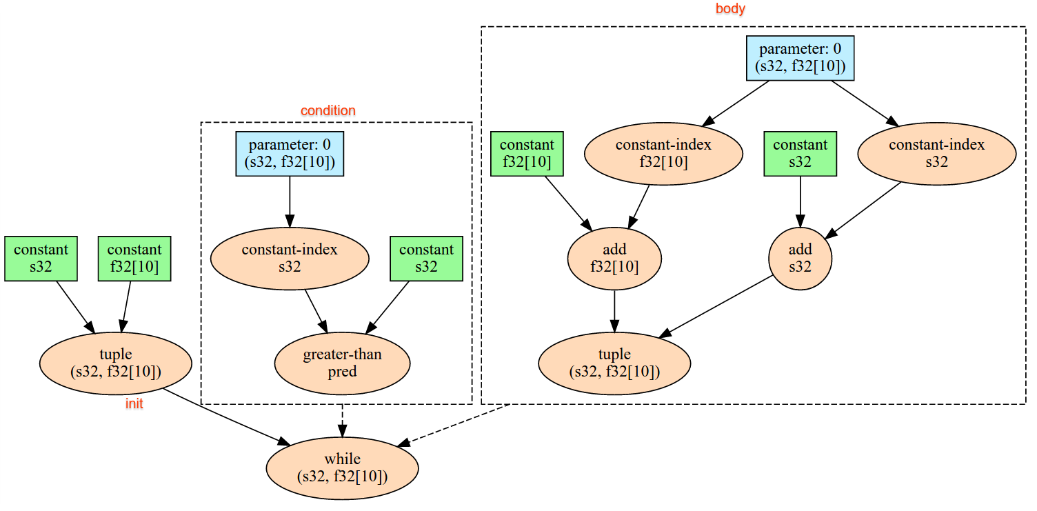
यह डिवाइस के इंप्लिसिट इनफ़ीड स्ट्रीमिंग इंटरफ़ेस से एक डेटा आइटम को पढ़ता है, डेटा को दिए गए आकार और उसके लेआउट के हिसाब से समझता है. साथ ही, डेटा का XlaOp नतीजे के तौर पर दिखाता है. कंप्यूटेशन में एक से ज़्यादा इनफ़ीड कार्रवाइयों की अनुमति है, लेकिन इनफ़ीड कार्रवाइयों में एक क्रम होना चाहिए. उदाहरण
के लिए, नीचे दिए गए कोड में मौजूद दो 'इनफ़ीड' का कुल क्रम है, क्योंकि
'टाइम लूप' के बीच निर्भरता होती है.
result1 = while (condition, init = init_value) {
  Infeed(shape)
}

result2 = while (condition, init = result1) {
  Infeed(shape)
}
नेस्ट किए गए टपल आकार काम नहीं करते. खाली टपल आकार के लिए, इनफ़ीड ऑपरेशन में कोई रुकावट नहीं होती है और यह डिवाइस के Infeed से किसी भी डेटा को पढ़े बिना आगे बढ़ जाता है.
आयोटा
XlaBuilder::Iota
भी देखें.
Iota(shape, iota_dimension)
यह किसी बड़े होस्ट ट्रांसफ़र के बजाय, डिवाइस पर एक स्थिर लिटरल
बनाने में मदद करता है. एक ऐसा अरे बनाता है जिसमें तय आकार होता है. साथ ही, शून्य से शुरू होने वाली और तय डाइमेंशन के साथ एक की बढ़ोतरी करके वैल्यू रखता है. फ़्लोटिंग-पॉइंट टाइप के लिए, बनाया गया कलेक्शन ConvertElementType(Iota(...)) के बराबर है, जहां Iota इंटिग्रल टाइप की है और कन्वर्ज़न फ़्लोटिंग-पॉइंट टाइप में है.
| तर्क | टाइप | सिमैंटिक |
|---|---|---|
shape |
Shape |
Iota() के बनाए गए कलेक्शन का आकार |
iota_dimension |
int64 |
वह डाइमेंशन जिसे साथ-साथ बढ़ाना है. |
उदाहरण के लिए, Iota(s32[4, 8], 0) आइटम लौटाएं
  [[0, 0, 0, 0, 0, 0, 0, 0 ],
   [1, 1, 1, 1, 1, 1, 1, 1 ],
   [2, 2, 2, 2, 2, 2, 2, 2 ],
   [3, 3, 3, 3, 3, 3, 3, 3 ]]
Iota(s32[4, 8], 1) तक के प्रॉडक्ट लौटाएं
  [[0, 1, 2, 3, 4, 5, 6, 7 ],
   [0, 1, 2, 3, 4, 5, 6, 7 ],
   [0, 1, 2, 3, 4, 5, 6, 7 ],
   [0, 1, 2, 3, 4, 5, 6, 7 ]]
मैप
XlaBuilder::Map
भी देखें.
Map(operands..., computation)
| तर्क | टाइप | सिमैंटिक |
|---|---|---|
operands |
N XlaOp सेकंड का क्रम |
T0..T{N-1} टाइप की N कैटगरी |
computation |
XlaComputation |
आर्बिट्रेरी टाइप के T और M टाइप के N पैरामीटर के साथ, T_0, T_1, .., T_{N + M -1} -> S टाइप का कैलकुलेशन |
dimensions |
int64 कलेक्शन |
मैप डाइमेंशन का कलेक्शन |
दी गई operands सरणियों पर एक अदिश फ़ंक्शन लागू करता है, जो एक जैसे डाइमेंशन का एक अरे बनाता है जहां हर एलिमेंट, इनपुट सरणियों में संबंधित एलिमेंट पर लागू किए गए मैप किए गए फ़ंक्शन का नतीजा होता है.
मैप किया गया फ़ंक्शन, पाबंदी के साथ आर्बिट्रेरी कैलकुलेशन है. इसमें अदिश टाइप T के N इनपुट और टाइप S वाला सिंगल आउटपुट है. आउटपुट में वही डाइमेंशन होते हैं जो ऑपरेंड के होते हैं. हालांकि, T टाइप को एलिमेंट S से बदल दिया जाता है.
उदाहरण के लिए: Map(op1, op2, op3, computation, par1), आउटपुट कलेक्शन बनाने के लिए इनपुट ऐरे में मौजूद हर (मल्टी-डाइमेंशन) इंडेक्स पर elem_out <-
computation(elem1, elem2, elem3, par1) को मैप करता है.
OptimizationBarrier
किसी भी ऑप्टिमाइज़ेशन पास को रुकावट के पार कंप्यूटेशन से ले जाने से रोकता है.
यह पक्का करता है कि सभी इनपुट का आकलन, ऐसे किसी भी ऑपरेटर से पहले किया जाए जो रुकावट के आउटपुट पर निर्भर है.
पैड
XlaBuilder::Pad
भी देखें.
Pad(operand, padding_value, padding_config)
| तर्क | टाइप | सिमैंटिक |
|---|---|---|
operand |
XlaOp |
T टाइप की कैटगरी |
padding_value |
XlaOp |
जोड़ी गई पैडिंग (जगह) भरने के लिए, T टाइप का स्केलर |
padding_config |
PaddingConfig |
हर डाइमेंशन के एलिमेंट के दोनों किनारों (कम, ज़्यादा) और एलिमेंट के बीच पैडिंग (जगह) की संख्या |
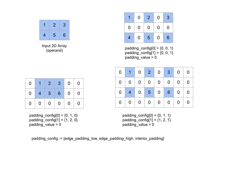
अरे के साथ-साथ दिए गए padding_value वाले ऐरे के एलिमेंट के बीच पैडिंग करके, दिए गए operand अरे को बड़ा करता है. padding_config
हर डाइमेंशन के लिए, किनारे की पैडिंग (जगह) और अंदरूनी पैडिंग (जगह) की जानकारी देता है.
PaddingConfig, PaddingConfigDimension का दोहराया गया फ़ील्ड है, जिसमें हर डाइमेंशन के लिए तीन फ़ील्ड होते हैं: edge_padding_low, edge_padding_high, और
interior_padding.
edge_padding_low और edge_padding_high, हर डाइमेंशन के लो-एंड (इंडेक्स 0 के बगल में) और हाई-एंड (सबसे बड़े इंडेक्स के बगल में) में जोड़ी गई पैडिंग की संख्या बताते हैं. एज पैडिंग की मात्रा ऋणात्मक हो सकती है --
ऋणात्मक पैडिंग का कुल मान, तय किए गए डाइमेंशन से हटाए जाने वाले एलिमेंट की संख्या बताता है.
interior_padding हर डाइमेंशन में, किसी भी दो एलिमेंट के बीच जोड़ी गई पैडिंग (जगह) की जानकारी देता है. हालांकि, यह नेगेटिव नहीं हो सकता. इंटीरियर पैडिंग, एज पैडिंग के पहले लॉजिकल तरीके से होती है. इसलिए, नेगेटिव एज पैडिंग के मामले में, एलिमेंट को इंटीरियर-पैडेड ऑपरेंड से हटा दिया जाता है.
अगर एज पैडिंग के सभी पेयर (0, 0) हैं और
अंदरूनी पैडिंग की वैल्यू 0 है, तो यह कार्रवाई ज़रूरी नहीं है. नीचे दी गई इमेज में, दो डाइमेंशन वाले कलेक्शन के लिए edge_padding और interior_padding अलग-अलग वैल्यू के उदाहरण दिए गए हैं.
रिकव
XlaBuilder::Recv
भी देखें.
Recv(shape, channel_handle)
| तर्क | टाइप | सिमैंटिक |
|---|---|---|
shape |
Shape |
पाने के लिए डेटा का आकार |
channel_handle |
ChannelHandle |
भेजे/रिकवरी के हर जोड़े के लिए यूनीक आइडेंटिफ़ायर |
दिए गए आकार का डेटा, उसी चैनल का हैंडल शेयर करने वाले दूसरे कंप्यूटेशन में Send निर्देश से लेता है. मिले डेटा के लिए
XlaOp दिखाता है.
Recv कार्रवाई का Client API, सिंक्रोनस कम्यूनिकेशन दिखाता है.
हालांकि, एसिंक्रोनस डेटा ट्रांसफ़र को चालू करने के लिए, निर्देश को अंदरूनी तौर पर एचएलओ के दो निर्देशों
(Recv और RecvDone) में बांटा जाता है. HloInstruction::CreateRecv और HloInstruction::CreateRecvDone भी देखें.
Recv(const Shape& shape, int64 channel_id)
एक ही channel_id वाले Send निर्देश से डेटा पाने के लिए ज़रूरी संसाधन बांटता है. दिए गए संसाधनों का संदर्भ देता है, जिसका इस्तेमाल नीचे दिए गए RecvDone निर्देश के ज़रिए किया जाता है और डेटा ट्रांसफ़र पूरा होने का इंतज़ार किया जाता है. कॉन्टेक्स्ट, {पाएं buffer (आकार), अनुरोध आइडेंटिफ़ायर
(U32)} का टपल है और इसका इस्तेमाल सिर्फ़ RecvDone निर्देश के साथ किया जा सकता है.
RecvDone(HloInstruction context)
Recv निर्देश के हिसाब से बनाए गए कॉन्टेक्स्ट को ध्यान में रखते हुए, डेटा ट्रांसफ़र की प्रोसेस पूरी होने का इंतज़ार किया जाता है और मिले डेटा को दिखाया जाता है.
खराब कॉन्टेंट को फ़ैलने से रोकना
XlaBuilder::Reduce
भी देखें.
साथ-साथ, एक या उससे ज़्यादा कलेक्शन पर कम करने वाला फ़ंक्शन लागू करता है.
Reduce(operands..., init_values..., computation, dimensions)
| तर्क | टाइप | सिमैंटिक |
|---|---|---|
operands |
N XlaOp का क्रम |
T_0, ..., T_{N-1} टाइप की N कैटगरी. |
init_values |
N XlaOp का क्रम |
T_0, ..., T_{N-1} टाइप के N स्केलर. |
computation |
XlaComputation |
T_0, ..., T_{N-1}, T_0, ..., T_{N-1} -> Collate(T_0, ..., T_{N-1}) टाइप की कैलकुलेशन. |
dimensions |
int64 कलेक्शन |
डाइमेंशन की बिना क्रम वाली कैटगरी का इस्तेमाल करें. |
जगह:
- N को 1 से बड़ा या उसके बराबर होना ज़रूरी है.
- कंप्यूटेशन को "मोटे तौर पर" असोसिएट होना चाहिए (नीचे देखें).
- सभी इनपुट ऐरे के डाइमेंशन एक जैसे होने चाहिए.
- सभी शुरुआती वैल्यू को
computationके तहत एक आइडेंटिटी बनानी होगी. - अगर
N = 1,Collate(T),Tहोता है. - अगर
N > 1है, तोCollate(T_0, ..., T_{N-1}),Tटाइप केNएलिमेंट का एक टपल है.
यह कार्रवाई हर इनपुट ऐरे के एक या उससे ज़्यादा डाइमेंशन को स्केलर में कम कर देती है.
दिखाई गई हर कैटगरी की रैंक rank(operand) - len(dimensions) है. ऑप का आउटपुट Collate(Q_0, ..., Q_N) है, जहां Q_i T_i टाइप की कैटगरी है. डाइमेंशन के बारे में नीचे बताया गया है.
अलग-अलग बैकएंड को सीमित करने की गणना को फिर से जोड़ने की अनुमति है. इससे संख्याओं में अंतर हो सकता है, क्योंकि कम करने वाले कुछ फ़ंक्शन, फ़्लोट के लिए सहयोगी नहीं होते हैं. हालांकि, अगर डेटा की रेंज सीमित है, तो फ़्लोटिंग-पॉइंट जोड़ने की प्रोसेस, ज़्यादातर व्यावहारिक इस्तेमाल के लिए मददगार होती है.
उदाहरण
जब रिडक्शन फ़ंक्शन f (यह computation है) और [10, 11,
12, 13] वैल्यू वाली एक 1D कलेक्शन में किसी एक डाइमेंशन को कम किया जाता है, तो इसे इस तरह से कैलकुलेट किया जा सकता है
f(10, f(11, f(12, f(init_value, 13)))
हालांकि, और भी कई संभावनाएं हैं, जैसे कि
f(init_value, f(f(10, f(init_value, 11)), f(f(init_value, 12), f(init_value, 13))))
यहां एक छद्म कोड का उदाहरण दिया गया है. इसमें बताया गया है कि रिडक्शन को कैसे लागू किया जा सकता है. इसके लिए, योग को कम करने की प्रोसेस के तौर पर 0 की शुरुआती वैल्यू के साथ जोड़ना होता है.
result_shape <- remove all dims in dimensions from operand_shape

# Iterate over all elements in result_shape. The number of r's here is equal
# to the rank of the result
for r0 in range(result_shape[0]), r1 in range(result_shape[1]), ...:
  # Initialize this result element
  result[r0, r1...] <- 0

  # Iterate over all the reduction dimensions
  for d0 in range(dimensions[0]), d1 in range(dimensions[1]), ...:
    # Increment the result element with the value of the operand's element.
    # The index of the operand's element is constructed from all ri's and di's
    # in the right order (by construction ri's and di's together index over the
    # whole operand shape).
    result[r0, r1...] += operand[ri... di]
यहां 2D ऐरे (मैट्रिक्स) को कम करने का एक उदाहरण दिया गया है. आकृति की रैंक 2 है, डाइमेंशन 0 का साइज़ 2 है, और डाइमेंशन 1 है:
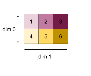
"जोड़ें" फ़ंक्शन से डाइमेंशन 0 या 1 को कम करने के नतीजे:
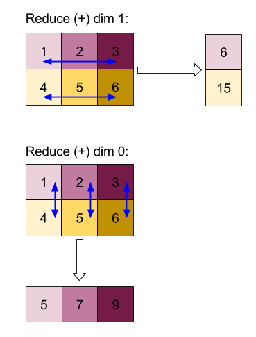
ध्यान दें कि दोनों कमी के नतीजे 1D अरे हैं. इस डायग्राम में दिखाया गया है कि एक को कॉलम के तौर पर दिखाया गया है और दूसरे को पंक्ति के तौर पर.
ज़्यादा जटिल उदाहरण के लिए, यहां 3D कलेक्शन दिया गया है. इसकी रैंक 3 है, साइज़ 4 की डाइमेंशन 0 है, साइज़ 2 का डाइमेंशन 1 है, और साइज़ 3 का डाइमेंशन 2 है. आसानी के लिए, 1 से 6 तक की वैल्यू को 0 डाइमेंशन में दोहराया जाता है.
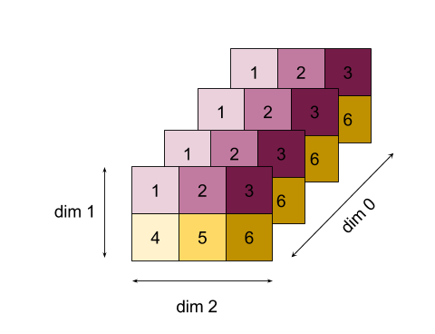
इसी तरह, 2D उदाहरण की तरह, हम सिर्फ़ एक डाइमेंशन को कम कर सकते हैं. उदाहरण के लिए, अगर हम डाइमेंशन 0 को कम करते हैं, तो हमें रैंक-2 का अरे मिलता है जिसमें डाइमेंशन 0 की सभी वैल्यू एक स्केलर में फ़ोल्ड हो जाती हैं:
|  4   8  12 |
| 16  20  24 |
अगर हम डाइमेंशन 2 को कम करते हैं, तो हमें रैंक-2 वाला अरे भी मिलता है, जहां डाइमेंशन 2 की सभी वैल्यू एक स्केलर में फ़ोल्ड हो जाती हैं:
| 6  15 |
| 6  15 |
| 6  15 |
| 6  15 |
ध्यान दें कि इनपुट में बचे हुए डाइमेंशन के बीच मिलता-जुलता ऑर्डर, आउटपुट में सुरक्षित रहता है. हालांकि, हो सकता है कि कुछ डाइमेंशन को नई संख्या असाइन की जा सके (क्योंकि रैंक में बदलाव होता है).
हम एक से ज़्यादा डाइमेंशन को भी कम कर सकते हैं. डाइमेंशन 0 और 1 को कम करने से,
1D अरे [20, 28, 36] बनता है.
3D अरे को इसके सभी डाइमेंशन में कम करने से अदिश 84 बनता है.
वैरैडिक कम करें
N > 1 के बाद, 'कम करें' फ़ंक्शन को लागू करना थोड़ा मुश्किल होता है, क्योंकि यह सभी इनपुट पर एक साथ लागू होता है. ऑपरेंड, कंप्यूटेशन को
इस क्रम में दिए जाते हैं:
- पहले ऑपरेंड के लिए कम की गई वैल्यू चलाई जा रही है
- ...
- N'वें ऑपरेंड के लिए कम किया गया मान चल रहा है
- पहले ऑपरेंड के लिए इनपुट वैल्यू
- ...
- N'वें ऑपरेंड के लिए इनपुट वैल्यू
उदाहरण के लिए, नीचे दिए गए रिडक्शन फ़ंक्शन पर विचार करें, जिसका इस्तेमाल साथ-साथ 1-D ऐरे के सबसे बड़ी और तर्क की वैल्यू को कैलकुलेट करने के लिए किया जा सकता है:
f: (Float, Int, Float, Int) -> Float, Int
f(max, argmax, value, index):
  if value >= max:
    return (value, index)
  else:
    return (max, argmax)
1-D इनपुट ऐरे V = Float[N], K = Int[N] और इनिट वैल्यू
I_V = Float, I_K = Int के लिए, एक ही इनपुट डाइमेंशन में
घटाने का नतीजा f_(N-1) बार-बार होने वाले इस ऐप्लिकेशन के बराबर होता है:
f_0 = f(I_V, I_K, V_0, K_0)
f_1 = f(f_0.first, f_0.second, V_1, K_1)
...
f_(N-1) = f(f_(N-2).first, f_(N-2).second, V_(N-1), K_(N-1))
वैल्यू के अरे और क्रम में चलने वाले इंडेक्स (जैसे कि iota) की कैटगरी पर इस कमी को लागू करने पर, यह अरे पर फिर से लागू होगा. साथ ही, ज़्यादा से ज़्यादा वैल्यू और मेल खाने वाले इंडेक्स वाला टपल दिखेगा.
ReducePrecision
XlaBuilder::ReducePrecision
भी देखें.
फ़्लोटिंग-पॉइंट वैल्यू को कम सटीक फ़ॉर्मैट (जैसे कि IEEE-FP16) में बदलने और वापस ओरिजनल फ़ॉर्मैट में बदलने के असर को मॉडल करता है. कम सटीक फ़ॉर्मैट में, एक्सपोनेंट और मैंटिसा बिट की संख्या, मन मुताबिक तय की जा सकती है. हालांकि, हो सकता है कि सभी बिट साइज़, हर तरह के हार्डवेयर इंप्लीमेंटेशन पर काम न करते हों.
ReducePrecision(operand, mantissa_bits, exponent_bits)
| तर्क | टाइप | सिमैंटिक |
|---|---|---|
operand |
XlaOp |
फ़्लोटिंग-पॉइंट टाइप T की कैटगरी. |
exponent_bits |
int32 |
कम सटीक फ़ॉर्मैट में घातांक बिट की संख्या |
mantissa_bits |
int32 |
कम सटीक फ़ॉर्मैट में मैंटिससा बिट की संख्या |
नतीजा, T टाइप की एक कैटगरी है. इनपुट वैल्यू को मेंटिसा बिट की दी गई संख्या ("सम उससे जुड़ी संख्या" सिमैंटिक का इस्तेमाल करके) के सबसे करीबी
वैल्यू से राउंड ऑफ़ किया जाता है. साथ ही, कोई भी ऐसी वैल्यू जो घातांक बिट की संख्या से तय की गई सीमा से ज़्यादा होती है, उसे पॉज़िटिव या नेगेटिव अनगिनत कर दिया जाता है. NaN वैल्यू बनी रहती हैं. हालांकि, इन्हें कैननिकल NaN वैल्यू में बदला जा सकता है.
कम से कम सटीक फ़ॉर्मैट में कम से कम एक घातांक बिट होना चाहिए (शून्य से वैल्यू में अंतर करने के लिए, क्योंकि दोनों में मैंटिसा ज़ीरो होता है). साथ ही, इसमें मैंटिसा बिट की संख्या गैर-ऋणात्मक होनी चाहिए. घातांक (एक्सपोनेंट) या
मैंटिसा बिट की संख्या, टाइप T के हिसाब से तय की गई वैल्यू से ज़्यादा हो सकती है. ऐसे में, कन्वर्ज़न का संबंधित हिस्सा 'नो-ऑप' होगा.
ReduceScatter
XlaBuilder::ReduceScatter
भी देखें.
LookScatter एक साथ मिलकर की जाने वाली कार्रवाई है, जो All होती है. यह नतीजे को
scatter_dimension के साथ-साथ shard_count ब्लॉक में बांटकर, नतीजे को स्कैटर करती है और रेप्लिका ग्रुप में मौजूद रेप्लिका i को ith शॉर्टकट में बांटती है.
ReduceScatter(operand, computation, scatter_dim, shard_count,
replica_group_ids, channel_id)
| तर्क | टाइप | सिमैंटिक |
|---|---|---|
operand |
XlaOp |
दोहरावों को कम करने के लिए, अरे या अरे का ऐसा टपल जो खाली न हो. |
computation |
XlaComputation |
रिडक्शन कंप्यूटेशन |
scatter_dimension |
int64 |
स्कैटर के लिए डाइमेंशन. |
shard_count |
int64 |
scatter_dimension को बांटने के लिए ब्लॉक की संख्या |
replica_groups |
int64 के वेक्टर का वेक्टर |
वे ग्रुप जिनके बीच में कमी की जाती है |
channel_id |
वैकल्पिक int64 |
क्रॉस-मॉड्यूल कम्यूनिकेशन के लिए वैकल्पिक चैनल आईडी |
- जब
operand, अरे का टपल है, तो टपल के हर एलिमेंट पर रिड्यूस-स्कैटर फ़ंक्शन लागू किया जाता है. replica_groupsउन प्रतिरूप समूहों की सूची है जिनके बीच कमी की जाती है (मौजूदा प्रतिरूप के लिए रेप्लिका आईडीReplicaIdका इस्तेमाल करके फिर से पाया जा सकता है). हर ग्रुप में प्रतिरूपों का क्रम तय करता है कि पूरे कम करने के नतीजे किस क्रम में दिखेंगे.replica_groupsखाली होना चाहिए (जिस स्थिति में सभी रेप्लिका एक ही ग्रुप से जुड़े हैं) या उसमें उतने ही एलिमेंट होने चाहिए जितने रेप्लिका की संख्या में हैं. अगर एक से ज़्यादा रेप्लिका ग्रुप मौजूद हैं, तो उन सभी का साइज़ एक ही होना चाहिए. उदाहरण के लिए,replica_groups = {0, 2}, {1, 3},0और2, और1और3के बीच कम जानकारी देता है. इसके बाद, नतीजे को बिगाड़ता है.shard_countहर कॉपी ग्रुप का साइज़ होता है. हमें इसकी ज़रूरत तब होती है, जबreplica_groupsखाली हो. अगरreplica_groupsखाली नहीं है, तोshard_countहर डुप्लीकेट ग्रुप के साइज़ के बराबर होना चाहिए.channel_idका इस्तेमाल, क्रॉस-मॉड्यूल कम्यूनिकेशन के लिए किया जाता है: एक हीchannel_idवालेreduce-scatterऑपरेशन ही एक-दूसरे से कम्यूनिकेट कर सकते हैं.
आउटपुट साइज़, इनपुट का आकार होता है. इसमें scatter_dimension को
shard_count गुना छोटा किया जाता है. उदाहरण के लिए, अगर दो रेप्लिका हैं और
ऑपरेंड की वैल्यू [1.0, 2.25] है और
ऑपरेंड की वैल्यू [3.0, 5.25] है, तो इस ऑपर्च्यूनिटी की आउटपुट वैल्यू जहां scatter_dim है, वहां पहली कॉपी के लिए [4.0] और दूसरी रेप्लिका के लिए [7.5] होगा.0
ReduceWindow
XlaBuilder::ReduceWindow
भी देखें.
N बहु-आयामी सरणियों के अनुक्रम की हर विंडो में मौजूद सभी एलिमेंट पर रिडक्शन फ़ंक्शन लागू करता है, जो आउटपुट के रूप में N बहु-आयामी सरणियों का एक या टपल बनाता है. हर आउटपुट अरे में एलिमेंट की संख्या और विंडो की मान्य स्थितियों की संख्या बराबर होती है. पूल की गई लेयर को ReduceWindow के तौर पर दिखाया जा सकता है. Reduce की तरह ही, लागू किया गया computation हमेशा बाईं ओर मौजूद init_values के पास होता है.
ReduceWindow(operands..., init_values..., computation, window_dimensions,
window_strides, padding)
| तर्क | टाइप | सिमैंटिक |
|---|---|---|
operands |
N XlaOps |
T_0,..., T_{N-1} टाइप की N मल्टी-डाइमेंशनल रेंज का क्रम. इसमें हर वह बेस एरिया दिखाता है जिस पर विंडो रखी गई है. |
init_values |
N XlaOps |
कमी के लिए N शुरुआती वैल्यू, हर N ऑपरेंड के लिए एक. ज़्यादा जानकारी के लिए, कम करें पर जाएं. |
computation |
XlaComputation |
सभी इनपुट ऑपरेंड की हर विंडो में मौजूद एलिमेंट पर लागू करने के लिए, T_0, ..., T_{N-1}, T_0, ..., T_{N-1} -> Collate(T_0, ..., T_{N-1}) टाइप का रिडक्शन फ़ंक्शन. |
window_dimensions |
ArraySlice<int64> |
विंडो की डाइमेंशन वैल्यू के लिए पूर्णांकों का कलेक्शन |
window_strides |
ArraySlice<int64> |
विंडो स्ट्राइड वैल्यू के लिए पूर्णांकों का कलेक्शन |
base_dilations |
ArraySlice<int64> |
बेस फ़ैलेशन वैल्यू के लिए पूर्णांकों का कलेक्शन |
window_dilations |
ArraySlice<int64> |
विंडो डाइलेशन वैल्यू के लिए पूर्णांकों का कलेक्शन |
padding |
Padding |
विंडो के लिए पैडिंग टाइप (Pपैडिंग::ksame), इसका मतलब है कि स्ट्राइड 1 होने पर, इनपुट के जैसा आउटपुट आकार रखें या पैडिंग::kValid, जो पैडिंग (जगह) का इस्तेमाल नहीं करता है और विंडो के फ़िट न होने पर उसे "बंद" कर देता है) |
जगह:
- N को 1 से बड़ा या उसके बराबर होना ज़रूरी है.
- सभी इनपुट ऐरे के डाइमेंशन एक जैसे होने चाहिए.
- अगर
N = 1,Collate(T),Tहोता है. - अगर
N > 1है, तोCollate(T_0, ..., T_{N-1}),(T0,...T{N-1})टाइप केNएलिमेंट का एक टपल है.
नीचे दिए गए कोड और इमेज में, ReduceWindow को इस्तेमाल करने का एक उदाहरण दिया गया है. इनपुट,
साइज़ [4x6] का मैट्रिक्स है. साथ ही, window_डाइमेंशनs और window_stride_डाइमेंशन, दोनों [2x3] होते हैं.
// Create a computation for the reduction (maximum).
XlaComputation max;
{
  XlaBuilder builder(client_, "max");
  auto y = builder.Parameter(0, ShapeUtil::MakeShape(F32, {}), "y");
  auto x = builder.Parameter(1, ShapeUtil::MakeShape(F32, {}), "x");
  builder.Max(y, x);
  max = builder.Build().value();
}

// Create a ReduceWindow computation with the max reduction computation.
XlaBuilder builder(client_, "reduce_window_2x3");
auto shape = ShapeUtil::MakeShape(F32, {4, 6});
auto input = builder.Parameter(0, shape, "input");
builder.ReduceWindow(
    input,
    /*init_val=*/builder.ConstantLiteral(LiteralUtil::MinValue(F32)),
    *max,
    /*window_dimensions=*/{2, 3},
    /*window_stride_dimensions=*/{2, 3},
    Padding::kValid);
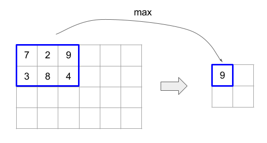
किसी डाइमेंशन में 1 होने पर, यह पता चलता है कि डाइमेंशन में किसी विंडो की जगह उसके पास वाली विंडो से 1 एलिमेंट दूर है. यह बताने के लिए कि कोई भी विंडो एक-दूसरे से ओवरलैप नहीं कर रही है, window_stride_dimensions, window_dimensions के बराबर होना चाहिए. नीचे दी गई इमेज में, स्ट्राइड के दो अलग-अलग वैल्यू का इस्तेमाल दिखाया गया है. इनपुट के हर डाइमेंशन पर पैडिंग (जगह) लागू की जाती है और कैलकुलेशन की प्रोसेस एक जैसी होती हैं.
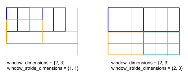
एक नॉन-ट्रिवियल पैडिंग उदाहरण के लिए, डाइमेंशन 3 के साथ कम से कम विंडो (शुरुआती वैल्यू MAX_FLOAT है) और इनपुट ऐरे [10000, 1000, 100, 10, 1] पर 2 को घुमाएं. इस तरह के पैडिंग (जगह) का इस्तेमाल करने पर विचार करें. kValid की पैडिंग, कम से कम दो मान्य विंडो से की जाती है: [10000, 1000, 100] और [100, 10, 1]. इससे, आउटपुट [100, 1] मिलता है. kSame को पैडिंग करने पर, सबसे पहले अरे को पैड किया जाता है, ताकि कम विंडो के बाद की आकार, स्ट्राइड वन के इनपुट के समान ही हो. ऐसा, दोनों तरफ़ शुरुआती एलिमेंट जोड़कर किया जाता है, जिससे [MAX_VALUE, 10000, 1000, 100, 10, 1,
MAX_VALUE] मिलता है. पैडेड ऐरे पर कम विंडो चलाने की सुविधा तीन विंडो [MAX_VALUE, 10000, 1000], [1000, 100, 10], [10, 1, MAX_VALUE], और यील्ड [1000, 10, 1] पर काम करती है.
कम करने के फ़ंक्शन का आकलन करने का क्रम मनचाहे तरीके से
हो सकता है और यह तय नहीं होता. इसलिए, कम करने के फ़ंक्शन को फिर से जोड़ने के लिए बहुत ज़्यादा संवेदनशील नहीं होना चाहिए. ज़्यादा जानकारी के लिए, Reduce के संदर्भ में असोसिएशन के बारे में हुई चर्चा देखें.
ReplicaId
XlaBuilder::ReplicaId
भी देखें.
प्रतिरूप का यूनीक आईडी (U32 अदिश) दिखाता है.
ReplicaId()
हर नकल का यूनीक आईडी, [0, N) इंटरवल में साइन नहीं किया गया एक पूर्णांक होता है. इसमें N, कॉपी की संख्या होती है. सभी रेप्लिका एक ही प्रोग्राम को चला रहे हैं, इसलिए प्रोग्राम में ReplicaId() कॉल हर रेप्लिका के लिए अलग वैल्यू दिखाएगा.
आकार बदलें
XlaBuilder::Reshape और Collapse कार्रवाई भी देखें.
किसी ऐरे के डाइमेंशन को नए कॉन्फ़िगरेशन में बदलता है.
Reshape(operand, new_sizes)
Reshape(operand, dimensions, new_sizes)
| तर्क | टाइप | सिमैंटिक |
|---|---|---|
operand |
XlaOp |
T टाइप की कैटगरी |
dimensions |
int64 वेक्टर |
डाइमेंशन को छोटा करने का क्रम |
new_sizes |
int64 वेक्टर |
नए डाइमेंशन के साइज़ का वेक्टर |
सैद्धांतिक तौर पर, पहले किसी अरे को डेटा वैल्यू के एक-डाइमेंशन वाले वेक्टर में बदल देता है
और फिर इस वेक्टर को नए आकार में बदल देता है. इनपुट आर्ग्युमेंट, T टाइप का एक आर्बिट्रेरी अरे है, जो डाइमेंशन इंडेक्स का कंपाइल-टाइम-कॉन्सटेंट वेक्टर है. नतीजे के लिए, डाइमेंशन साइज़ का कंपाइल-टाइम-कॉन्सटेंट वेक्टर है.
अगर dimension वेक्टर में वैल्यू दी गई है, तो यह T के सभी डाइमेंशन का क्रमचय होना चाहिए. अगर वैल्यू नहीं दी गई है, तो {0, ..., rank - 1} है. dimensions में डाइमेंशन का क्रम, सबसे धीरे बदलने वाले डाइमेंशन (सबसे बड़ा) से लेकर लूप नेस्ट में सबसे तेज़ बदलने वाले डाइमेंशन (सबसे छोटा) तक होता है. यह इनपुट ऐरे को एक डाइमेंशन में छोटा कर देता है. new_sizes वेक्टर, आउटपुट ऐरे का साइज़ तय करता है. new_sizes में इंडेक्स 0 की वैल्यू, डाइमेंशन 0 का साइज़, इंडेक्स 1 की वैल्यू, डाइमेंशन 1 का साइज़ वगैरह होती है. new_size डाइमेंशन का प्रॉडक्ट, ऑपरेंड के डाइमेंशन साइज़ के प्रॉडक्ट के बराबर होना चाहिए. छोटा किए गए अरे को new_sizes से तय किए गए मल्टीडाइमेंशन कलेक्शन में रिफ़ाइन करते समय, new_sizes में डाइमेंशन को सबसे कम और सबसे कम अंतर (सबसे कम) से सबसे कम क्रम में लगाया जाता है.
उदाहरण के लिए, v को 24 एलिमेंट की कैटगरी बनाएं:
let v = f32[4x2x3] { { {10, 11, 12}, {15, 16, 17} },
                    { {20, 21, 22}, {25, 26, 27} },
                    { {30, 31, 32}, {35, 36, 37} },
                    { {40, 41, 42}, {45, 46, 47} } };

In-order collapse:
let v012_24 = Reshape(v, {0,1,2}, {24});
then v012_24 == f32[24] {10, 11, 12, 15, 16, 17, 20, 21, 22, 25, 26, 27,
                         30, 31, 32, 35, 36, 37, 40, 41, 42, 45, 46, 47};

let v012_83 = Reshape(v, {0,1,2}, {8,3});
then v012_83 == f32[8x3] { {10, 11, 12}, {15, 16, 17},
                          {20, 21, 22}, {25, 26, 27},
                          {30, 31, 32}, {35, 36, 37},
                          {40, 41, 42}, {45, 46, 47} };

Out-of-order collapse:
let v021_24 = Reshape(v, {1,2,0}, {24});
then v012_24 == f32[24]  {10, 20, 30, 40, 11, 21, 31, 41, 12, 22, 32, 42,
                          15, 25, 35, 45, 16, 26, 36, 46, 17, 27, 37, 47};

let v021_83 = Reshape(v, {1,2,0}, {8,3});
then v021_83 == f32[8x3] { {10, 20, 30}, {40, 11, 21},
                          {31, 41, 12}, {22, 32, 42},
                          {15, 25, 35}, {45, 16, 26},
                          {36, 46, 17}, {27, 37, 47} };


let v021_262 = Reshape(v, {1,2,0}, {2,6,2});
then v021_262 == f32[2x6x2] { { {10, 20}, {30, 40},
                              {11, 21}, {31, 41},
                              {12, 22}, {32, 42} },
                             { {15, 25}, {35, 45},
                              {16, 26}, {36, 46},
                              {17, 27}, {37, 47} } };
खास मामले में, रीशेप किसी सिंगल-एलिमेंट अरे को अदिश में बदल सकता है और इससे उलटा भी कर सकता है. उदाहरण के लिए,
Reshape(f32[1x1] { {5} }, {0,1}, {}) == 5;
Reshape(5, {}, {1,1}) == f32[1x1] { {5} };
रेव (रिवर्स)
XlaBuilder::Rev
भी देखें.
Rev(operand, dimensions)
| तर्क | टाइप | सिमैंटिक |
|---|---|---|
operand |
XlaOp |
T टाइप की कैटगरी |
dimensions |
ArraySlice<int64> |
रिवर्स करने के लिए डाइमेंशन |
operand कलेक्शन में मौजूद एलिमेंट के क्रम को उलटा करता है. साथ ही, तय किए गए
dimensions फ़ंक्शन के हिसाब से एक ही आकार का आउटपुट अरे जनरेट करता है. मल्टीडाइमेंशन वाले इंडेक्स में, ऑपरेंड अरे का हर एलिमेंट, बदले गए इंडेक्स में आउटपुट कलेक्शन में सेव होता है. मल्टी-डाइमेंशनल इंडेक्स को हर डाइमेंशन में इंडेक्स को उलटा करके बदल दिया जाता है. यानी, अगर साइज़ N वाला डाइमेंशन, रिवर्सिंग डाइमेंशन में से एक है, तो उसका इंडेक्स i, N - 1 - i में बदल जाता है.
Rev ऑपरेशन के लिए एक इस्तेमाल, न्यूरल नेटवर्क में ग्रेडिएंट कंप्यूटेशन के दौरान दो विंडो डाइमेंशन के साथ कॉन्वलूशन वेट अरे को रिवर्स करना होता है.
RngNormal
XlaBuilder::RngNormal
भी देखें.
सामान्य डिस्ट्रिब्यूशन \(N(\mu, \sigma)\) के बाद जनरेट हुई रैंडम संख्याओं से किसी दिए गए आकार का आउटपुट बनाता है. पैरामीटर \(\mu\) , \(\sigma\), और आउटपुट आकार में फ़्लोटिंग पॉइंट एलिमेंटल टाइप होना चाहिए. इसके अलावा, पैरामीटर का स्केलर मान होना चाहिए.
RngNormal(mu, sigma, shape)
| तर्क | टाइप | सिमैंटिक |
|---|---|---|
mu |
XlaOp |
जनरेट की गई संख्याओं का माध्य तय करने वाला T प्रकार का स्केलर |
sigma |
XlaOp |
T प्रकार का स्केलर, जो जनरेट किए गए का स्टैंडर्ड डीविएशन तय करता है |
shape |
Shape |
T टाइप के आउटपुट का आकार |
RngUniform
XlaBuilder::RngUniform
भी देखें.
इंटरवल \([a,b)\)पर एक जैसे डिस्ट्रिब्यूशन के बाद जनरेट हुई रैंडम संख्याओं के साथ किसी दिए गए आकार का आउटपुट बनाता है. पैरामीटर और आउटपुट एलिमेंट का टाइप बूलियन टाइप, इंटिग्रल टाइप या फ़्लोटिंग पॉइंट टाइप होना चाहिए. साथ ही, उसके टाइप एक जैसे होने चाहिए. फ़िलहाल, सीपीयू और जीपीयू बैकएंड में सिर्फ़ F64, F32, F16, BF16, S64, U64, S32, और U32 का इस्तेमाल किया जा सकता है. इसके अलावा, पैरामीटर की वैल्यू अदिश वैल्यू होनी चाहिए. अगर \(b <= a\) नतीजे के तौर पर लागू करने के तरीके के बारे में बताया गया है.
RngUniform(a, b, shape)
| तर्क | टाइप | सिमैंटिक |
|---|---|---|
a |
XlaOp |
T प्रकार का स्केलर, जिसमें अंतराल की निचली सीमा तय की गई है |
b |
XlaOp |
अंतराल की ऊपरी सीमा तय करने वाला T प्रकार का स्केलर |
shape |
Shape |
T टाइप के आउटपुट का आकार |
RngBitGenerator
तय किए गए एल्गोरिदम (या बैकएंड डिफ़ॉल्ट) का इस्तेमाल करके, दिए गए आकार के साथ एक जैसे रैंडम बिट से आउटपुट जनरेट करता है. साथ ही, अपडेट की गई स्थिति (जिसकी शुरुआती स्थिति का आकार है) और जनरेट किए गए रैंडम डेटा का इस्तेमाल करके, अपडेट की गई स्थिति दिखाता है.
शुरुआती स्थिति, रैंडम नंबरों को जनरेट करने वाले मौजूदा नंबर की शुरुआती स्थिति होती है. यह और ज़रूरी आकार और मान्य वैल्यू, इस्तेमाल किए गए एल्गोरिदम पर निर्भर करती हैं.
इस बात की गारंटी है कि आउटपुट शुरुआती स्थिति का डिटर्मिनिस्टिक फ़ंक्शन होगा. हालांकि, इसकी गारंटी नहीं है कि बैकएंड और अलग-अलग कंपाइलर वर्शन के बीच यह फ़ंक्शन तय होगा.
RngBitGenerator(algorithm, key, shape)
| तर्क | टाइप | सिमैंटिक |
|---|---|---|
algorithm |
RandomAlgorithm |
पीआरएनजी एल्गोरिदम का इस्तेमाल किया जाना चाहिए. |
initial_state |
XlaOp |
PRNG एल्गोरिदम की शुरुआती स्थिति. |
shape |
Shape |
जनरेट किए गए डेटा के लिए आउटपुट आकार. |
algorithm के लिए उपलब्ध वैल्यू:
rng_default: बैकएंड की खास आकार की शर्तों के साथ खास एल्गोरिदम.rng_three_fry: थ्री फ़्राई काउंटर-आधारित पीआरएनजी एल्गोरिदम.initial_stateआकार आर्बिट्रेरी वैल्यू वालाu64[2]है. सैलमन और अन्य एससी 2011. पैरलल रैंडम नंबर: 1, 2, 3 जितने आसान होते हैं.rng_philox: साथ-साथ रैंडम नंबर जनरेट करने के लिए Philox एल्गोरिदम.initial_stateका आकार,u64[3]है. इसमें आर्बिट्रेरी वैल्यू का इस्तेमाल किया गया है. सैलमन और अन्य एससी 2011. पैरलल रैंडम नंबर: 1, 2, 3 जितने आसान होते हैं.
स्कैटर
XLA स्कैटर ऑपरेशन, नतीजों का एक क्रम जनरेट करता है, जो इनपुट ऐरे operands की वैल्यू होते हैं. इसमें कई स्लाइस (scatter_indices के बताए गए इंडेक्स पर) होते हैं, जिन्हें update_computation का इस्तेमाल करके, updates में वैल्यू के क्रम के साथ अपडेट किया जाता है.
XlaBuilder::Scatter
भी देखें.
scatter(operands..., scatter_indices, updates..., update_computation,
index_vector_dim, update_window_dims, inserted_window_dims,
scatter_dims_to_operand_dims)
| तर्क | टाइप | सिमैंटिक |
|---|---|---|
operands |
N XlaOp का क्रम |
N कैटगरी की ऐसी कैटगरी जिन्हें T_0, ..., T_N में फैलाया जाना है. |
scatter_indices |
XlaOp |
वह कलेक्शन जिसमें उन स्लाइस के शुरुआती इंडेक्स हैं जिन्हें आस-पास होना चाहिए. |
updates |
N XlaOp का क्रम |
T_0, ..., T_N टाइप की N कैटगरी. updates[i] में ऐसी वैल्यू होती हैं जिनका इस्तेमाल operands[i] को स्कैटर करने के लिए किया जाना चाहिए. |
update_computation |
XlaComputation |
इनपुट ऐरे में मौजूद वैल्यू और स्कैटर के दौरान अपडेट को एक साथ जोड़ने के लिए इस्तेमाल किया जाने वाला कंप्यूटेशन. यह कंप्यूटेशन, T_0, ..., T_N, T_0, ..., T_N -> Collate(T_0, ..., T_N) टाइप का होना चाहिए. |
index_vector_dim |
int64 |
scatter_indices में मौजूद वह डाइमेंशन जिसमें शुरुआती इंडेक्स शामिल हैं. |
update_window_dims |
ArraySlice<int64> |
updates के आकार में डाइमेंशन का सेट, जो विंडो के डाइमेंशन होते हैं. |
inserted_window_dims |
ArraySlice<int64> |
विंडो डाइमेंशन का सेट, जिसे updates के आकार में शामिल किया जाना चाहिए. |
scatter_dims_to_operand_dims |
ArraySlice<int64> |
डाइमेंशन मैप, स्कैटर इंडेक्स से ऑपरेंड इंडेक्स स्पेस तक होता है. इस कलेक्शन को i को scatter_dims_to_operand_dims[i] में मैप करने के तौर पर इस्तेमाल किया जाता है . इसे वन-टू-वन और कुल होना चाहिए. |
indices_are_sorted |
bool |
क्या इंडेक्स, कॉलर के हिसाब से क्रम में लगाए जाने की गारंटी है. |
जगह:
- N को 1 से बड़ा या उसके बराबर होना ज़रूरी है.
operands[0], ...,operands[N-1] सभी के डाइमेंशन एक जैसे होने चाहिए.updates[0], ...,updates[N-1] सभी के डाइमेंशन एक जैसे होने चाहिए.- अगर
N = 1,Collate(T),Tहोता है. - अगर
N > 1है, तोCollate(T_0, ..., T_N),Tटाइप केNएलिमेंट का एक टपल है.
अगर index_vector_dim, scatter_indices.rank के बराबर है, तो हम अनुमान के तौर पर
scatter_indices को ट्रेलिंग 1 डाइमेंशन मानते हैं.
हम ArraySlice<int64> टाइप के update_scatter_dims को updates के आकार वाले डाइमेंशन के सेट के तौर पर बताते हैं. ये ऐसे डाइमेंशन होते हैं जो update_window_dims में नहीं होते. ये बढ़ते क्रम में होते हैं.
स्कैटर के तर्कों को इन कंस्ट्रेंट का पालन करना चाहिए:
हर
updatesकलेक्शन की रैंकupdate_window_dims.size + scatter_indices.rank - 1होनी चाहिए.हर
updatesकलेक्शन में डाइमेंशनiकी सीमाएं, इन शर्तों के मुताबिक होनी चाहिए:- अगर
update_window_dimsमेंiमौजूद है (जैसे कि कुछkके लिएupdate_window_dims[k] के बराबर), तोupdatesमें डाइमेंशनiकी सीमा,inserted_window_dims(उदाहरण के लिए,adjusted_window_bounds[k] को शामिल करने के बाद,operandकी संबंधित सीमा से ज़्यादा नहीं होनी चाहिए). यहांadjusted_window_bounds, इंडेक्स पर सीमाओं के साथoperandकी सीमाएंinserted_window_dimsहटा दी गई है. - अगर
update_scatter_dimsमेंiमौजूद है (जैसे, कुछkके लिएupdate_scatter_dims[k] के बराबर), तोupdatesमेंiकी सीमा,scatter_indicesकी संबंधित बाउंड के बराबर होनी चाहिए. इसमेंindex_vector_dim(जैसे,scatter_indices.shape.dims[k] को छोड़ने पर,k<index_vector_dimऔरscatter_indices.shape.dims[k+1] को छोड़ा जा सकता है).
- अगर
update_window_dims, बढ़ते क्रम में होना चाहिए. साथ ही, इसमें दोहराया गया डाइमेंशन नंबर नहीं होना चाहिए. साथ ही, यह[0, updates.rank)रेंज में होना चाहिए.inserted_window_dims, बढ़ते क्रम में होना चाहिए. साथ ही, इसमें दोहराया गया डाइमेंशन नंबर नहीं होना चाहिए. साथ ही, यह[0, operand.rank)रेंज में होना चाहिए.operand.rank,update_window_dims.sizeऔरinserted_window_dims.sizeके योग के बराबर होना चाहिए.scatter_dims_to_operand_dims.size,scatter_indices.shape.dims[index_vector_dim] के बराबर होना चाहिए और इसकी वैल्यू[0, operand.rank)की रेंज में होनी चाहिए.
हर updates कलेक्शन में दिए गए इंडेक्स U के लिए, operands कलेक्शन में मौजूद इंडेक्स I को इस तरह कैलकुलेट किया जाता है:
- मान लें कि
update_scatter_dims} मेंkके लिए,G= {U[k] है.scatter_indicesकलेक्शन में इंडेक्स वेक्टरSपता करने के लिए,Gका इस्तेमाल करें. इससेS[i] =scatter_indices[मिलाएं(G,i)] इस तरह लिखें कि काॅपीराइट(A, b),index_vector_dimकी स्थितियों में b को A में डाल देता है. scatter_dims_to_operand_dimsमैप का इस्तेमाल करकेSस्कैटर करके,Sका इस्तेमाल करकेoperandमेंSinइंडेक्स बनाएं. औपचारिक तौर पर:Sin[scatter_dims_to_operand_dims[k]] =S[k], अगरk<scatter_dims_to_operand_dims.size.Sin[_] =0अन्य मामलों में.
- हर
operandsकलेक्शन में, इंडेक्सWinबनाएं. इसके लिए,Uमेंupdate_window_dimsपर इंडेक्स कोinserted_window_dimsके हिसाब से फैलाएं. औपचारिक तौर पर:Win[window_dims_to_operand_dims(k)] =U[k] अगरkupdate_window_dimsमें है, तो यहांwindow_dims_to_operand_dims, [0,update_window_dims.size) और रेंज [0,operand.rank) \inserted_window_dimsवाला मोनोटोनिक फ़ंक्शन है. (उदाहरण के लिए, अगरupdate_window_dims.size,4है,operand.rank6है, औरinserted_window_dims{0,2} है, तोwindow_dims_to_operand_dims{0→1,1→3,2→4,3→5} है).Win[_] =0अन्य मामलों में.
I,Win+Sinहै, जहां +, एलिमेंट के हिसाब से जोड़ा गया है.
खास जानकारी में, स्कैटर ऑपरेशन को इस तरह परिभाषित किया जा सकता है.
outputकी शुरुआतoperandsके साथ करें. इसका मतलब है कि सभी इंडेक्सJके लिए,operands[J] कलेक्शन में मौजूद सभी इंडेक्सOके लिए:
output[J][O] =operands[J][O]updates[J] कलेक्शन में मौजूद हर इंडेक्सUऔरoperand[J] कलेक्शन में मौजूदOके इंडेक्स के लिए, अगरO,outputके लिए मान्य इंडेक्स है:
(output[0][O], ...,output[N-1][O]) =update_computation(output[0][O], ..., ,output[N-1][O],updates[0][U], ...,updates[N-1][U])
अपडेट लागू होने का क्रम तय नहीं होता है. इसलिए, जब updates में एक से ज़्यादा इंडेक्स, operands के एक ही इंडेक्स को रेफ़र करते हैं, तो output में संबंधित वैल्यू तय नहीं होगी.
ध्यान दें कि update_computation में दिया गया पहला पैरामीटर
हमेशा output कलेक्शन की मौजूदा वैल्यू होगी और दूसरा पैरामीटर
हमेशा updates कलेक्शन की वैल्यू होगी. यह खास तौर पर उन मामलों में ज़रूरी है, जब update_computation क्रम से नहीं बदला जा सकता.
अगर indices_are_sorted को 'सही' पर सेट किया जाता है, तो XLA यह मान सकता है कि उपयोगकर्ता ने start_indices को
बढ़ते start_index_map के क्रम में लगाया है. अगर ऐसा नहीं है,
तो सिमैंटिक लागू किया जाता है.
अनौपचारिक तौर पर, स्कैटर ऑप को कलेक्ट ऑप के इनवर्स के तौर पर देखा जा सकता है, यानी कि स्कैटर ऑप इनपुट में उन एलिमेंट को अपडेट करता है जो उससे जुड़े कलेक्ट ऑप से एक्सट्रैक्ट किए जाते हैं.
ज़्यादा जानकारी और उदाहरणों के लिए, Gather में
"अनौपचारिक जानकारी" सेक्शन देखें.
चुनें
XlaBuilder::Select
भी देखें.
प्रेडिकेट अरे की वैल्यू के आधार पर, दो इनपुट ऐरे के एलिमेंट से आउटपुट अरे बनाता है.
Select(pred, on_true, on_false)
| तर्क | टाइप | सिमैंटिक |
|---|---|---|
pred |
XlaOp |
PRED टाइप की कैटगरी |
on_true |
XlaOp |
T टाइप की कैटगरी |
on_false |
XlaOp |
T टाइप की कैटगरी |
on_true और on_false कैटगरी का आकार एक ही होना चाहिए. यह आउटपुट अरे का आकार भी होता है. PRED एलिमेंट टाइप के साथ, pred कैटगरी की डाइमेंशन on_true और on_false के बराबर होनी चाहिए.
pred के हर एलिमेंट P के लिए, आउटपुट ऐरे का संबंधित एलिमेंट
on_true से लिया जाता है. अगर P की वैल्यू true है, तो on_false से और P की वैल्यू false होने पर, उससे जुड़ा एलिमेंट लिया जाता है. ब्रॉडकास्ट करना के प्रतिबंधित तरीके के तौर पर, pred, PRED टाइप का स्केलर हो सकता है. इस मामले में, अगर pred true है, तो आउटपुट ऐरे को पूरी तरह से on_true से लिया जाता है. साथ ही, अगर pred false है, तो on_false से लिया जाता है.
नॉन-स्केलर pred के साथ उदाहरण:
let pred: PRED[4] = {true, false, false, true};
let v1: s32[4] = {1, 2, 3, 4};
let v2: s32[4] = {100, 200, 300, 400};
==>
Select(pred, v1, v2) = s32[4]{1, 200, 300, 4};
अदिश pred के साथ उदाहरण:
let pred: PRED = true;
let v1: s32[4] = {1, 2, 3, 4};
let v2: s32[4] = {100, 200, 300, 400};
==>
Select(pred, v1, v2) = s32[4]{1, 2, 3, 4};
ट्यूपल के बीच चुनने की सुविधा काम करती है. इस काम के लिए टपल को अदिश
टाइप माना जाता है. अगर on_true और on_false टूपल (जिनका आकार
एक ही होना चाहिए!) है, तो pred को PRED टाइप का स्केलर होना चाहिए.
SelectAndScatter
XlaBuilder::SelectAndScatter
भी देखें.
इस ऑपरेशन को कंपोज़िट ऑपरेशन के तौर पर माना जाता है जो सबसे पहले हर विंडो से कोई एलिमेंट चुनने के लिए, operand कलेक्शन पर ReduceWindow की गिनती करता है. इसके बाद, चुने गए एलिमेंट के इंडेक्स पर source अरे को फैला देता है, ताकि ऑपरेंड अरे के आकार वाली आउटपुट ऐरे को तैयार किया जा सके. बाइनरी select फ़ंक्शन का इस्तेमाल, हर विंडो से एक एलिमेंट चुनने के लिए किया जाता है. इसके लिए, इसे हर विंडो पर लागू किया जाता है. साथ ही, इसे ऐसी प्रॉपर्टी के साथ कॉल किया जाता है जिसमें पहले पैरामीटर का इंडेक्स वेक्टर, दूसरे पैरामीटर के इंडेक्स वेक्टर की तुलना में लेक्सिक तौर पर कम होता है. अगर पहला पैरामीटर चुना जाता है, तो select फ़ंक्शन true दिखाता है और दूसरा पैरामीटर चुनने पर false दिखाता है. साथ ही, फ़ंक्शन की ट्रांज़िटिविटी होनी चाहिए (जैसे, अगर select(a, b) और select(b, c) true हैं, तो select(a, c) भी true है), ताकि चुना गया एलिमेंट किसी दी गई विंडो में ले जाने वाले एलिमेंट के क्रम पर निर्भर न हो.
आउटपुट कलेक्शन में, चुने गए हर इंडेक्स पर scatter फ़ंक्शन लागू किया जाता है. यह
दो स्केलर पैरामीटर लेता है:
- आउटपुट कलेक्शन में चुने गए इंडेक्स पर मौजूदा वैल्यू
sourceसे मिली स्कैटर वैल्यू, जो चुने गए इंडेक्स पर लागू होती है
यह दोनों पैरामीटर को मिलाता है और एक स्केलर वैल्यू देता है. इसका इस्तेमाल आउटपुट ऐरे में चुने गए इंडेक्स
की वैल्यू को अपडेट करने के लिए किया जाता है. शुरुआत में, आउटपुट कलेक्शन के सभी इंडेक्स init_value पर सेट होते हैं.
आउटपुट अरे का आकार operand अरे और source ऐरे का आकार, operand अरे पर ReduceWindow
ऑपरेशन लागू करने से मिलने वाले नतीजे जैसा ही होना चाहिए. SelectAndScatter का इस्तेमाल, न्यूरल नेटवर्क में पूलिंग लेयर के लिए ग्रेडिएंट वैल्यू को बैकप्रोपेगेट करने के लिए किया जा सकता है.
SelectAndScatter(operand, select, window_dimensions, window_strides,
padding, source, init_value, scatter)
| तर्क | टाइप | सिमैंटिक |
|---|---|---|
operand |
XlaOp |
T प्रकार का अरे, जिस पर विंडो स्लाइड होती है |
select |
XlaComputation |
हर विंडो में सभी एलिमेंट पर लागू करने के लिए, T, T -> PRED टाइप का बाइनरी कंप्यूटेशन. अगर पहला पैरामीटर चुना जाता है, तो true दिखाता है. वहीं, दूसरा पैरामीटर चुने जाने पर false दिखाता है |
window_dimensions |
ArraySlice<int64> |
विंडो की डाइमेंशन वैल्यू के लिए पूर्णांकों का कलेक्शन |
window_strides |
ArraySlice<int64> |
विंडो स्ट्राइड वैल्यू के लिए पूर्णांकों का कलेक्शन |
padding |
Padding |
विंडो के लिए पैडिंग (जगह) टाइप (पैडिंग::ksame या Padding::kValid) |
source |
XlaOp |
स्कैटर के लिए वैल्यू के साथ T टाइप की कैटगरी |
init_value |
XlaOp |
आउटपुट कलेक्शन की शुरुआती वैल्यू के लिए, टाइप T का स्केलर वैल्यू |
scatter |
XlaComputation |
हर स्कैटर सोर्स एलिमेंट को उसके डेस्टिनेशन एलिमेंट के साथ लागू करने के लिए, T, T -> T टाइप की बाइनरी कंप्यूटेशन |
नीचे दी गई इमेज में SelectAndScatter को इस्तेमाल करने के उदाहरण दिए गए हैं. इसमें select
फ़ंक्शन, अपने सभी पैरामीटर में सबसे बड़ी वैल्यू की गिनती करता है. ध्यान दें कि जब विंडो ओवरलैप होती हैं, तो जैसा कि नीचे दी गई इमेज (2) में दिखाया गया है, operand कलेक्शन के इंडेक्स को अलग-अलग विंडो से कई बार चुना जा सकता है. इस इमेज में, वैल्यू 9 का एलिमेंट, दोनों टॉप विंडो (नीले और लाल) से चुना गया है और बाइनरी जोड़ने वाला scatter फ़ंक्शन, वैल्यू 8 (2 + 6) का आउटपुट एलिमेंट देता है.
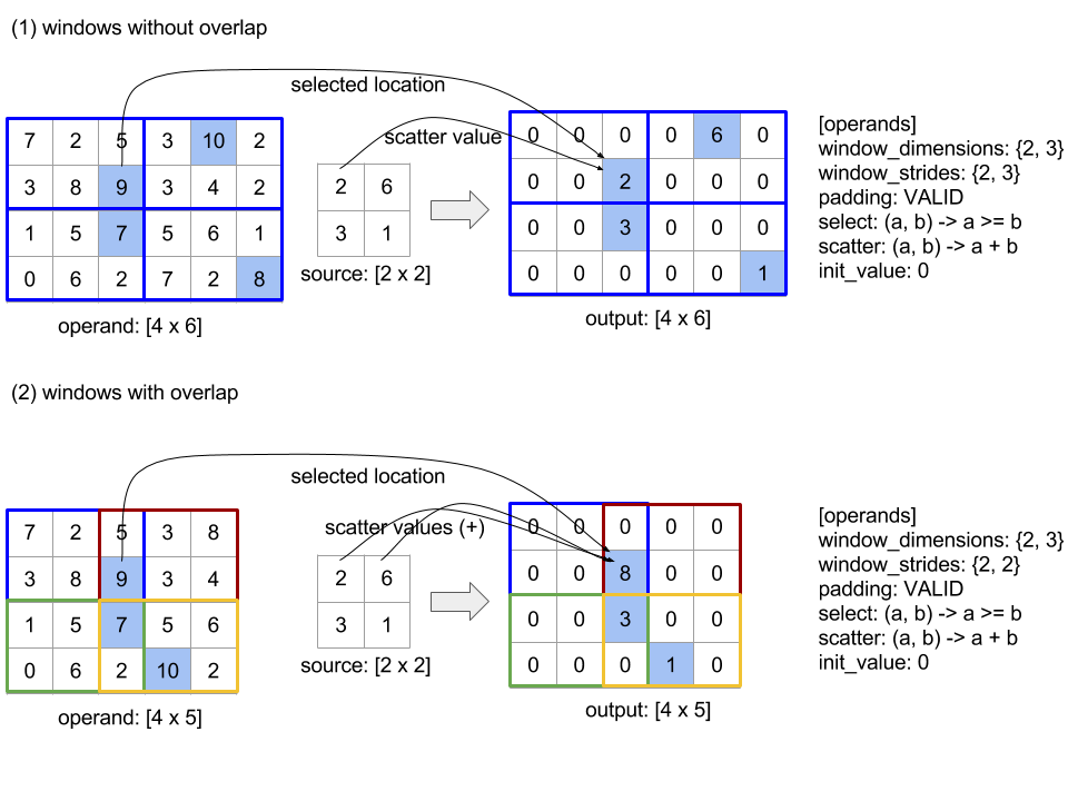
scatter फ़ंक्शन के आकलन का क्रम मनचाहे तरीके से तय होता है और हो सकता है कि यह तय न हो. इसलिए, scatter फ़ंक्शन को फिर से जोड़ने के लिए बहुत ज़्यादा संवेदनशील नहीं होना चाहिए. ज़्यादा जानकारी के लिए, Reduce के संदर्भ में असोसिएशन के बारे में हुई चर्चा देखें.
भेजें
XlaBuilder::Send
भी देखें.
Send(operand, channel_handle)
| तर्क | टाइप | सिमैंटिक |
|---|---|---|
operand |
XlaOp |
भेजा जाने वाला डेटा (T प्रकार की श्रेणी) |
channel_handle |
ChannelHandle |
भेजे/रिकवरी के हर जोड़े के लिए यूनीक आइडेंटिफ़ायर |
दिए गए ऑपरेंड डेटा को उसी चैनल हैंडल वाले अन्य कंप्यूटेशन में Recv निर्देश को भेजता है. कोई डेटा नहीं दिखाता.
Recv की तरह ही, Send कार्रवाई का क्लाइंट एपीआई, सिंक्रोनस कम्यूनिकेशन है. इसे एसिंक्रोनस डेटा ट्रांसफ़र को चालू करने के लिए, अंदरूनी तौर पर दो एचएलओ निर्देशों (Send और SendDone) में बांटा जाता है. HloInstruction::CreateSend और HloInstruction::CreateSendDone भी देखें.
Send(HloInstruction operand, int64 channel_id)
एक ही चैनल आईडी वाले Recv निर्देश से मिले संसाधनों पर ऑपरेंड का एसिंक्रोनस ट्रांसफ़र शुरू करता है. डेटा ट्रांसफ़र पूरा होने का इंतज़ार करने के लिए, कॉन्टेक्स्ट SendDone के निर्देश का इस्तेमाल करता है. कॉन्टेक्स्ट, {operand (आकार), अनुरोध पहचानकर्ता
(U32)} का एक टपल है और इसका इस्तेमाल सिर्फ़ SendDone निर्देश के ज़रिए किया जा सकता है.
SendDone(HloInstruction context)
Send निर्देश के ज़रिए बनाए गए कॉन्टेक्स्ट को ध्यान में रखते हुए, डेटा ट्रांसफ़र की प्रोसेस पूरी होने का इंतज़ार किया जाता है. इस निर्देश से कोई डेटा नहीं मिलता.
चैनल के निर्देशों को शेड्यूल करना
हर चैनल (Recv, RecvDone,
Send, SendDone) के लिए, चारों निर्देशों का पालन करने का क्रम नीचे दिया गया है.
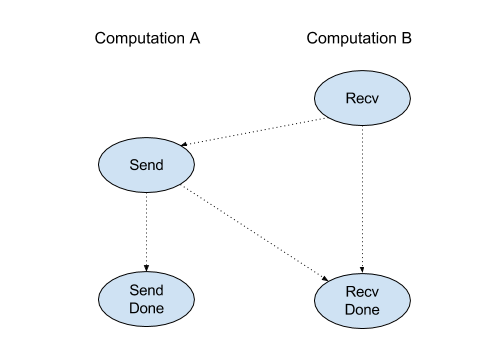
Recv,Sendसे पहले हैSend,RecvDoneसे पहले हैRecv,RecvDoneसे पहले हैSend,SendDoneसे पहले है
जब बैकएंड कंपाइलर, चैनल के निर्देशों की मदद से कम्यूनिकेट करने वाले हर कंप्यूटेशन के लिए एक लीनियर शेड्यूल जनरेट करते हैं, तब सभी कंप्यूटेशन पर एक साइकल नहीं होना चाहिए. उदाहरण के लिए, नीचे दिए गए शेड्यूल से डेडलॉक पैदा होते हैं.
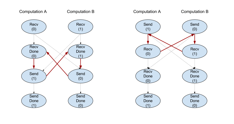
स्लाइस
XlaBuilder::Slice
भी देखें.
स्लाइसिंग, इनपुट अरे से सब-ऐरे को निकालता है. सब-ऐरे, उसी रैंक की होती है जो इनपुट में है. इसमें इनपुट ऐरे में, बाउंडिंग बॉक्स के अंदर वैल्यू शामिल होती हैं. यहां बाउंडिंग बॉक्स के डाइमेंशन और इंडेक्स, स्लाइस ऑपरेशन के लिए तर्क के तौर पर दिए जाते हैं.
Slice(operand, start_indices, limit_indices, strides)
| तर्क | टाइप | सिमैंटिक |
|---|---|---|
operand |
XlaOp |
T टाइप की N डाइमेंशन वाली अरे |
start_indices |
ArraySlice<int64> |
N पूर्णांक की सूची, जिसमें हर डाइमेंशन के स्लाइस के शुरुआती इंडेक्स मौजूद हैं. वैल्यू, शून्य से ज़्यादा या उसके बराबर होनी चाहिए. |
limit_indices |
ArraySlice<int64> |
हर डाइमेंशन के स्लाइस के लिए, आखिरी इंडेक्स (खास) वाले N पूर्णांक की सूची. हर वैल्यू, डाइमेंशन की start_indices वैल्यू से ज़्यादा या उसके बराबर होनी चाहिए. साथ ही, डाइमेंशन के साइज़ से कम या उसके बराबर होनी चाहिए. |
strides |
ArraySlice<int64> |
N पूर्णांक की सूची, जो स्लाइस के इनपुट स्ट्राइड को तय करती है. स्लाइस, d डाइमेंशन में हर strides[d] एलिमेंट को चुनता है. |
1-डाइमेंशन का उदाहरण:
let a = {0.0, 1.0, 2.0, 3.0, 4.0}
Slice(a, {2}, {4}) produces:
  {2.0, 3.0}
दो डाइमेंशन वाला उदाहरण:
let b =
 { {0.0,  1.0,  2.0},
   {3.0,  4.0,  5.0},
   {6.0,  7.0,  8.0},
   {9.0, 10.0, 11.0} }

Slice(b, {2, 1}, {4, 3}) produces:
  { { 7.0,  8.0},
    {10.0, 11.0} }
क्रम से लगाएं
XlaBuilder::Sort
भी देखें.
Sort(operands, comparator, dimension, is_stable)
| तर्क | टाइप | सिमैंटिक |
|---|---|---|
operands |
ArraySlice<XlaOp> |
क्रम से लगाए जाने वाले ऑपरेंड. |
comparator |
XlaComputation |
इस्तेमाल किया जाने वाला कंप्रेटर कंप्यूटेशन. |
dimension |
int64 |
वह डाइमेंशन जिसके साथ डेटा को क्रम से लगाना है. |
is_stable |
bool |
स्टेबल सॉर्टिंग का इस्तेमाल किया जाना चाहिए या नहीं. |
अगर सिर्फ़ एक ऑपरेंड दिया गया है, तो:
अगर ऑपरेंड रैंक-1 टेंसर (एक अरे) है, तो नतीजा क्रम से लगाया गया ऐरे होता है. अगर आपको अरे को बढ़ते क्रम में लगाना है, तो कंपैरेटर को तुलना से कम की परफ़ॉर्मेंस करनी चाहिए. आम तौर पर, अरे को क्रम से लगाने के बाद, यह
i < jवाले सभी इंडेक्स पोज़िशनi, jके लिए होल्ड पर रहता है, जिसमेंcomparator(value[i], value[j]) = comparator(value[j], value[i]) = falseयाcomparator(value[i], value[j]) = trueमें से कोई एक शामिल होता है.अगर ऑपरेंड की रैंक ज़्यादा है, तो ऑपरेंड को दिए गए डाइमेंशन के हिसाब से क्रम में लगाया जाता है. उदाहरण के लिए, रैंक-2 टेंसर (मैट्रिक्स) के लिए,
0की डाइमेंशन वैल्यू हर कॉलम को अलग-अलग क्रम में लगाएगी और1डाइमेंशन वैल्यू हर लाइन को अलग-अलग क्रम में लगाएगी. अगर कोई डाइमेंशन नंबर नहीं दिया जाता है, तो आखिरी डाइमेंशन को डिफ़ॉल्ट रूप से चुना जाता है. क्रम से लगाए गए डाइमेंशन के लिए, क्रम में लगाने का वही क्रम लागू होता है जो रैंक-1 के मामले में लागू होता है.
अगर n > 1 ऑपरेंड दिए गए हैं:
सभी
nऑपरेंड एक जैसे डाइमेंशन वाले टेंसर होने चाहिए. टेंसर के एलिमेंट टाइप अलग-अलग हो सकते हैं.सभी ऑपरेंड एक साथ क्रम से लगाए जाते हैं, अलग-अलग नहीं. सैद्धांतिक तौर पर, ऑपरेंड को एक टपल माना जाता है. यह जांच करते समय कि इंडेक्स की स्थितियों
iऔरjपर मौजूद हर ऑपरेंड के एलिमेंट को बदलने की ज़रूरत है या नहीं, कंपैरेटर को2 * nस्केलर पैरामीटर से कॉल किया जाता है, जहां पैरामीटर2 * k,k-thऑपरेंड की स्थितिiकी वैल्यू से जुड़ा होता है. साथ ही, पैरामीटर2 * k + 1,k-thऑपरेंड की पोज़िशनjकी वैल्यू से मेल खाता है. आम तौर पर, तुलना करने वाला टूल एक-दूसरे से2 * kऔर2 * k + 1पैरामीटर की तुलना करता है और टाई ब्रेकर के तौर पर दूसरे पैरामीटर पेयर का इस्तेमाल करता है.नतीजे में एक ऐसा टपल होता है जिसमें ऑपरेंड को क्रम से (जैसा कि ऊपर बताया गया है, दिए गए डाइमेंशन के साथ) शामिल होता है. टपल का
i-thऑपरेंड, क्रम केi-thऑपरेंड से मेल खाता है.
उदाहरण के लिए, अगर तीन ऑपरेंड operand0 = [3, 1],
operand1 = [42, 50], operand2 = [-3.0, 1.1] हैं, और कम्पैरेटर, सिर्फ़ operand0 की वैल्यू की तुलना इससे कम वाले वैल्यू के साथ करता है, तो क्रम में लगाने का आउटपुट
टपल ([1, 3], [50, 42], [1.1, -3.0]) होता है.
अगर is_stable को 'सही है' पर सेट किया जाता है, तो क्रम से लगाने के तरीके के स्थिर रहने की गारंटी दी जाती है. इसका मतलब है कि अगर
ऐसे एलिमेंट हैं जिन्हें तुलना करने वाले के हिसाब से बराबर माना जाता है, तो बराबर वैल्यू के क्रम को सुरक्षित रखा जाता है. दो एलिमेंट e1 और e2,
अगर और सिर्फ़ comparator(e1, e2) = comparator(e2, e1) = false होते हैं, तो बराबर होते हैं. डिफ़ॉल्ट रूप से, is_stable 'गलत' पर सेट होता है.
ट्रांसपोज़ करें
tf.reshape कार्रवाई भी देखें.
Transpose(operand)
| तर्क | टाइप | सिमैंटिक |
|---|---|---|
operand |
XlaOp |
ट्रांसपोज़ करने के लिए ऑपरेंड. |
permutation |
ArraySlice<int64> |
डाइमेंशन को अनुमति देने का तरीका. |
दिए गए क्रमचय के साथ ऑपरेंड डाइमेंशन की अनुमति देता है, इसलिए
∀ i . 0 ≤ i < rank ⇒ input_dimensions[permutation[i]] = output_dimensions[i].
यह रीशेप(ऑपरैंड, क्रमचय, परम्युटेशन(परम्यूटेशन, ऑपरेंड.शेप.डाइमेंशन)) की तरह ही होता है.
TriangularSolve
XlaBuilder::TriangularSolve
भी देखें.
कम या ऊपरी त्रिकोणीय गुणांकों वाले रैखिक समीकरणों की प्रणालियों को हल करने के लिए,
आगे या पीछे के प्रतिस्थापन की मदद लेता है. मुख्य डाइमेंशन के साथ ब्रॉडकास्ट करते हुए, यह रूटीन, वैरिएबल x के लिए एक मैट्रिक्स सिस्टम op(a) * x =
b या x * op(a) = b को हल करता है. इसमें a और b दिए गए हैं, जहां op(a), op(a) = a या op(a) = Transpose(a) या op(a) = Conj(Transpose(a)) है.
TriangularSolve(a, b, left_side, lower, unit_diagonal, transpose_a)
| तर्क | टाइप | सिमैंटिक |
|---|---|---|
a |
XlaOp |
रैंक > 2 की कैटगरी में आने वाले कॉम्प्लेक्स या फ़्लोटिंग-पॉइंट टाइप का अरे, जिसकी आकार [..., M, M] होती है. |
b |
XlaOp |
अगर left_side सही है, तो [..., M, K] आकार वाली एक ही रैंक > 2 वाली कैटगरी का अरे, नहीं तो [..., K, M] होगा. |
left_side |
bool |
यह बताता है कि op(a) * x = b (true) या x * op(a) = b (false) फ़ॉर्म के सिस्टम को हल करना है या नहीं. |
lower |
bool |
a के ऊपरी या निचले त्रिभुज का उपयोग करना है या नहीं. |
unit_diagonal |
bool |
अगर true है, तो a के विकर्ण एलिमेंट को 1 माना जाता है और इसे ऐक्सेस नहीं किया जाता है. |
transpose_a |
Transpose |
चाहे a का इस्तेमाल ऐसे ही करना हो, उसे ट्रांसपोज़ करना है या उसका कॉन्जुगेट ट्रांसपोज़ करना है. |
इनपुट डेटा को सिर्फ़ a के निचले/ऊपरी त्रिकोण से पढ़ा जाता है. हालांकि, यह lower की वैल्यू पर निर्भर करता है. दूसरे त्रिकोण के वैल्यू को नज़रअंदाज़ किया जाता है. आउटपुट डेटा
उसी त्रिभुज में दिखाया जाता है; दूसरे त्रिभुज में दी गई वैल्यू,
लागू करने से तय होती हैं और कुछ भी हो सकती हैं.
अगर a और b की रैंक, 2 से ज़्यादा है, तो उन्हें मैट्रिक्स के बैच के तौर पर माना जाता है.
इसमें मामूली दो डाइमेंशन को छोड़कर बाकी सभी डाइमेंशन बैच डाइमेंशन होते हैं. a और
b के बैच डाइमेंशन समान होने चाहिए.
टपल
XlaBuilder::Tuple
भी देखें.
ऐसा टपल जिसमें अलग-अलग संख्या में डेटा हैंडल होते हैं. हर हैंडल का अपना आकार होता है.
यह C++ में std::tuple के जैसा है. सैद्धांतिक तौर पर:
let v: f32[10] = f32[10]{0, 1, 2, 3, 4, 5, 6, 7, 8, 9};
let s: s32 = 5;
let t: (f32[10], s32) = tuple(v, s);
टपल को GetTupleElement कार्रवाई के ज़रिए, डीकंस्ट्रक्ट (ऐक्सेस किया जा सकता है) किया जा सकता है.
हालांकि
XlaBuilder::While
भी देखें.
While(condition, body, init)
| तर्क | टाइप | सिमैंटिक |
|---|---|---|
condition |
XlaComputation |
T -> PRED टाइप का XlaComप्यूटेशन, जो लूप खत्म होने की स्थिति को परिभाषित करता है. |
body |
XlaComputation |
T -> T टाइप का XlaComputation, जो लूप के मुख्य हिस्से को परिभाषित करता है. |
init |
T |
condition और body के पैरामीटर के लिए शुरुआती वैल्यू. |
condition के विफल होने तक body को क्रम से चलाता है. यह, कई दूसरी भाषाओं में आम तौर पर होने वाले लूप की तरह है. हालांकि, यहां दिए गए अंतर और पाबंदियों को छोड़कर.
WhileनोडTटाइप की वैल्यू दिखाता है, जोbodyके पिछले एक्ज़ीक्यूशन के बाद मिलता है.Tटाइप का आकार स्टैटिक रूप से तय किया जाता है और यह सभी बार में एक जैसा होना चाहिए.
कंप्यूटेशन के T पैरामीटर को पहली इटरेशन में init वैल्यू से शुरू किया जाता है और वे body के बाद के हर इटरेशन में, नए नतीजे में अपने-आप अपडेट हो जाते हैं.
While नोड का एक खास इस्तेमाल यह है कि न्यूरल नेटवर्क में ट्रेनिंग को बार-बार लागू किया जाए. सिंप्लिफ़ाइड स्यूडोकोड को यहां ग्राफ़ के साथ दिखाया गया है, जो कंप्यूटेशन को दिखाता है. यह कोड,
while_test.cc में देखा जा सकता है.
इस उदाहरण में दिया गया T टाइप, Tuple है. इसमें इटरेशन की गिनती के लिए int32 और इकट्ठार के लिए vector[10] शामिल हैं. 1,000 बार दोहराने के लिए, लूप
एक्यूमुलेटर में एक कॉन्सटेंट वेक्टर जोड़ता रहता है.
// Pseudocode for the computation.
init = {0, zero_vector[10]} // Tuple of int32 and float[10].
result = init;
while (result(0) < 1000) {
  iteration = result(0) + 1;
  new_vector = result(1) + constant_vector[10];
  result = {iteration, new_vector};
}