בהמשך מתוארת הסמנטיקה של פעולות המוגדרות בממשק XlaBuilder. בדרך כלל הפעולות האלה ממופות אחד לאחד לפעולות שמוגדרות בממשק RPC ב-xla_data.proto.
הערה לגבי מינוח: סוג הנתונים הכללי XLA מתמודד איתו הוא מערך ממדי N שמכיל רכיבים מסוג אחיד כלשהו (כמו מספר ממשי (float) ב-32 ביט. לאורך התיעוד, ה-array משמש לציון מערך ממדי שרירותי. לשם נוחות, למקרים מיוחדים יש שמות ספציפיים ומוכרים יותר. לדוגמה, וקטור הוא מערך חד-ממדי ומטריצה היא מערך דו-ממדי.
AfterAll
למידע נוסף: XlaBuilder::AfterAll.
חברת afterAll לוקחת מספר שונים של אסימונים ומפיקה אסימון יחיד. אסימונים הם סוגים פרימיטיביים שניתן לשרשר בין פעולות השפעה צדדיות כדי לאכוף את ביצוע ההזמנה. אפשר להשתמש בקוד AfterAll כצירוף אסימונים להזמנת פעולה אחרי פעולה שהוגדרה.
AfterAll(operands)
| ארגומנטים | סוג | סמנטיקה |
|---|---|---|
operands |
XlaOp |
מספר וריאנטים של אסימונים |
AllGather
למידע נוסף: XlaBuilder::AllGather.
מבצע שרשור בין רפליקות.
AllGather(operand, all_gather_dim, shard_count, replica_group_ids,
channel_id)
| ארגומנטים | סוג | סמנטיקה |
|---|---|---|
operand
|
XlaOp
|
מערך לשרשור בין עותקים |
all_gather_dim |
int64 |
מאפיין שרשור |
replica_groups
|
בווקטורים של int64 |
קבוצות שביניהן מתבצע השרשור |
channel_id
|
ערך אופציונלי של int64
|
מזהה ערוץ אופציונלי לתקשורת בין מודולים |
replica_groupsהיא רשימה של קבוצות העתקים שביניהן מתבצע שרשור (ניתן לאחזר מזהה עותק של ההעתק הנוכחי באמצעותReplicaId). סדר הרפליקות בכל קבוצה קובע את הסדר שבו ערכי הקלט שלהם ממוקמים בתוצאה.replica_groupsחייב להיות ריק (במקרה כזה, כל הרפליקות שייכות לקבוצה אחת, בסדר מ-0עדN - 1), או להכיל את אותו מספר רכיבים כמו מספר הרפליקות. לדוגמה, הקודreplica_groups = {0, 2}, {1, 3}מבצע שרשור בין הרפליקות0ו-2, ו-1ו-3.shard_countהוא הגודל של כל קבוצת עותקים. צריך להשתמש בה במקרים שבהם השדהreplica_groupsריק.channel_idמשמש לתקשורת בין מודולים: רק פעולותall-gatherעם אותוchannel_idיכולות לתקשר זו עם זו.
צורת הפלט היא צורת הקלט כאשר all_gather_dim גדל פי shard_count. לדוגמה, אם יש שתי רפליקות והאופרנד מכיל את הערך [1.0, 2.5] ו-[3.0, 5.25] בהתאמה בשתי הרפליקות, ערך הפלט מהפעולה הזו שבו all_gather_dim הוא 0 יהיה [1.0, 2.5, 3.0,
5.25] בשתי הרפליקות.
AllReduce
למידע נוסף: XlaBuilder::AllReduce.
מבצע חישוב מותאם אישית על פני רפליקות.
AllReduce(operand, computation, replica_group_ids, channel_id)
| ארגומנטים | סוג | סמנטיקה |
|---|---|---|
operand
|
XlaOp
|
מערך או צמד לא ריק של מערכים כדי לצמצם בין רפליקות |
computation |
XlaComputation |
חישוב הפחתה |
replica_groups
|
בווקטורים של int64 |
קבוצות שביניהן מתבצעות ההפחתה |
channel_id
|
ערך אופציונלי של int64
|
מזהה ערוץ אופציונלי לתקשורת בין מודולים |
- כשהערך הוא
operandב-tuple של מערכים, כל פונקציית ההפחתה מבוצעת בכל רכיב ב-tuple. replica_groupsהיא רשימה של קבוצות עותקים שביניהן מתבצעת ההפחתה (ניתן לאחזר מזהה עותק של הרפליקה הנוכחי באמצעותReplicaId). השדהreplica_groupsחייב להיות ריק (במקרה כזה, כל הרפליקות שייכות לקבוצה אחת) או להכיל את אותו מספר רכיבים כמו מספר הרפליקות. לדוגמה, הפונקציהreplica_groups = {0, 2}, {1, 3}מבצעת הפחתה בין הרפליקות0ו-2, ו-1ו-3.channel_idמשמש לתקשורת בין מודולים: רק פעולותall-reduceעם אותוchannel_idיכולות לתקשר זו עם זו.
צורת הפלט זהה לצורת הקלט. לדוגמה, אם יש שני
עותקים ולאופרנד יש את הערך [1.0, 2.5] ו-[3.0, 5.25]
בהתאמה בשני הרפליקות, ערך הפלט מהפעולה
והסיכום הזה יהיה [4.0, 7.75] בשני הרפליקות. אם הקלט נוצר ב-tuple, גם הפלט יופיע ב-tuple.
כדי לחשב את התוצאה של AllReduce צריך לקבל קלט אחד מכל עותק, כך שאם העתק אחד יבצע צומת AllReduce יותר פעמים מאשר עותק אחר, העותק הקודם ימתין לתמיד. כל הרפליקות פועלות באותה תוכנית, אז אין הרבה דרכים לעשות את זה, אבל יכול להיות שתנאי של לולאת בלולאה תלוי בנתונים מהפיד ובנתונים שמוזנים
וגורמים ללולאת הזמן לחזור יותר פעמים על רפליקה אחת ולא יותר.
AllToAll
למידע נוסף: XlaBuilder::AllToAll.
AllToAll היא פעולה קולקטיבית ששולחת נתונים מכל הליבות לכל הליבות. התהליך כולל שני שלבים:
- שלב הפיזור. בכל ליבה, האופרנד מחולק למספר
split_countשל בלוקים לאורךsplit_dimensions, והבלוקים מפוזרים לכל הליבות, למשל הבלוק it נשלח לליבת ה-ith. - שלב האיסוף. כל ליבה משורשרת את הבלוקים שהתקבלו לאורך
concat_dimension.
אפשר להגדיר את הליבות המשתתפות בתוכנית:
replica_groups: כל ReplicaGroup מכיל רשימה של מזהי עותקים שמשתתפים בחישוב (אפשר לאחזר את המזהה של העותק הנוכחי באמצעותReplicaId). AllToAll ייושם בתוך קבוצות המשנה לפי הסדר שצוין. לדוגמה, המשמעות שלreplica_groups = { {1,2,3}, {4,5,0} }היא ש-AllToAll ייושם בתוך רפליקות{1, 2, 3}, ובשלב האיסוף, והבלוקים שהתקבלו ישורשו באותו סדר של 1, 2, 3. לאחר מכן, יוחל AllToAll אחר בתוך רפליקות 4, 5 ו-0, וסדר השרשור הוא גם 4, 5, 0. אם השדהreplica_groupsריק, כל הרפליקות שייכות לקבוצה אחת, לפי סדר השרשור שבו הן מופיעות.
דרישות מוקדמות:
- גודל האופרנד ב-
split_dimensionמתחלק ב-split_count. - צורת האופרנד אינה כפולה.
AllToAll(operand, split_dimension, concat_dimension, split_count,
replica_groups)
| ארגומנטים | סוג | סמנטיקה |
|---|---|---|
operand |
XlaOp |
מערך קלט n ממדי |
split_dimension
|
int64
|
ערך באינטרוול [0,
n) שנותן שם למאפיין
שלאופרנד
שמפוצל |
concat_dimension
|
int64
|
ערך במרווח [0,
n) שנותן שם למאפיין
שלאורכו משורשרים הבלוקים המפוצלים |
split_count
|
int64
|
מספר הליבות שמשתתפות בפעולה הזו. אם השדה replica_groups ריק, הוא צריך להיות מספר העותקים הכפולים. אחרת, הוא צריך להיות שווה למספר הרפליקות בכל קבוצה. |
replica_groups
|
וקטור ReplicaGroup
|
כל קבוצה מכילה רשימה של מזהים כפולים. |
למטה מוצגת דוגמה של Alltoall.
XlaBuilder b("alltoall");
auto x = Parameter(&b, 0, ShapeUtil::MakeShape(F32, {4, 16}), "x");
AllToAll(x, /*split_dimension=*/1, /*concat_dimension=*/0, /*split_count=*/4);
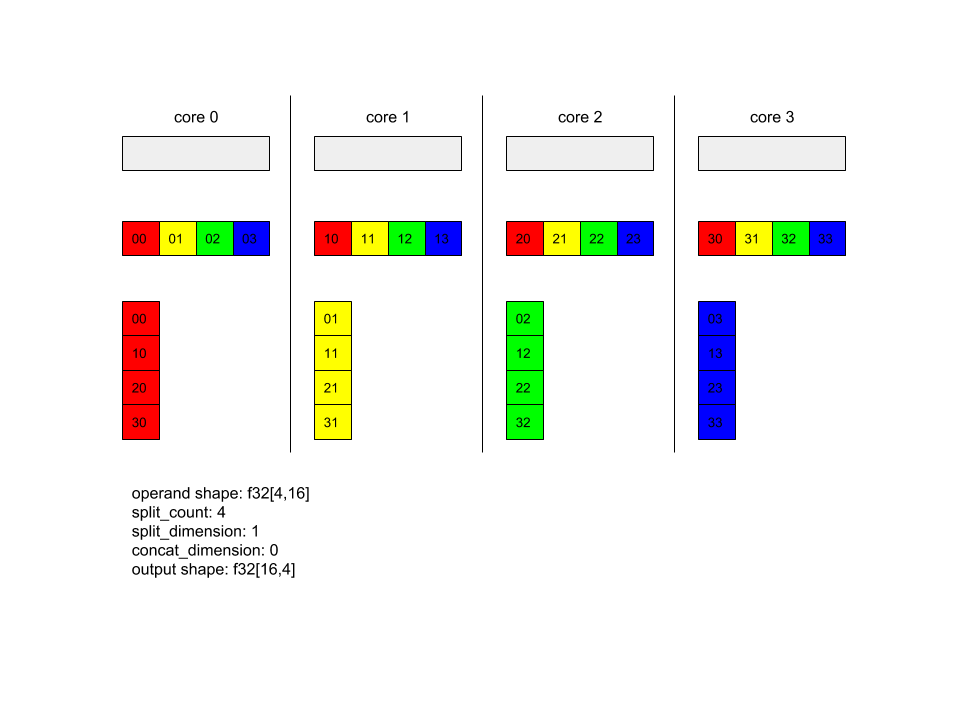
בדוגמה הזו יש 4 ליבות שמשתתפות ב-Alltoall. בכל ליבה, האופרנד מחולק לארבעה חלקים לאורך מימד 0, כך שלכל חלק יש צורה f32[4,4]. 4 החלקים מפוזרים לכל הליבות. לאחר מכן כל ליבה משורשרת את החלקים שהתקבלו לאורך מימד 1, לפי סדר ליבה 0-4. כך שהפלט של כל ליבה הוא בצורה f32[16,4].
BatchNormGrad
לתיאור מפורט של האלגוריתם, אפשר להיעזר ב-XlaBuilder::BatchNormGrad ובמאמר המקורי בנושא נורמליזציה רק על אצוות.
מחשבת את ההדרגתיות של הנורמה באצווה.
BatchNormGrad(operand, scale, mean, variance, grad_output, epsilon, feature_index)
| ארגומנטים | סוג | סמנטיקה |
|---|---|---|
operand |
XlaOp |
מערך n ממדי לנורמלי (x) |
scale |
XlaOp |
מערך דו-ממדי אחד (\(\gamma\)) |
mean |
XlaOp |
מערך דו-ממדי אחד (\(\mu\)) |
variance |
XlaOp |
מערך דו-ממדי אחד (\(\sigma^2\)) |
grad_output |
XlaOp |
הדרגתיים הועברו אל BatchNormTraining (\(\nabla y\)) |
epsilon |
float |
ערך אפסילון (\(\epsilon\)) |
feature_index |
int64 |
אינדקס למאפיין התכונה ב-operand |
לכל תכונה במאפיין התכונה (feature_index הוא האינדקס למאפיין התכונה ב-operand), הפעולה מחשבת את ההדרגתיות בהתאם ל-operand, ל-offset ול-scale בכל המאפיינים האחרים. הערך feature_index חייב להיות אינדקס חוקי למימד של התכונה ב-operand.
שלושת ההדרגות מוגדרים באמצעות הנוסחאות הבאות (בהנחה שמערך 4 ממדי הוא operand, ועם אינדקס מאפיין התכונה l, גודל אצווה m והגדלים המרחביים w ו-h):
\[ \begin{split} c_l&= \frac{1}{mwh}\sum_{i=1}^m\sum_{j=1}^w\sum_{k=1}^h \left( \nabla y_{ijkl} \frac{x_{ijkl} - \mu_l}{\sigma^2_l+\epsilon} \right) \\\\ d_l&= \frac{1}{mwh}\sum_{i=1}^m\sum_{j=1}^w\sum_{k=1}^h \nabla y_{ijkl} \\\\ \nabla x_{ijkl} &= \frac{\gamma_{l} }{\sqrt{\sigma^2_{l}+\epsilon} } \left( \nabla y_{ijkl} - d_l - c_l (x_{ijkl} - \mu_{l}) \right) \\\\ \nabla \gamma_l &= \sum_{i=1}^m\sum_{j=1}^w\sum_{k=1}^h \left( \nabla y_{ijkl} \frac{x_{ijkl} - \mu_l}{\sqrt{\sigma^2_{l}+\epsilon} } \right) \\\\\ \nabla \beta_l &= \sum_{i=1}^m\sum_{j=1}^w\sum_{k=1}^h \nabla y_{ijkl} \end{split} \]
הקלט mean ו-variance מייצגים ערכי רגעים במאפיינים של אצווה ומרחבי.
סוג הפלט מורכב מ-tuple של שלוש נקודות אחיזה:
| פלט | סוג | סמנטיקה |
|---|---|---|
grad_operand
|
XlaOp
|
הדרגתי ביחס לקלט operand ($\nabla
x$) |
grad_scale
|
XlaOp
|
הדרגתי ביחס לקלט scale ($\nabla
\gamma$) |
grad_offset
|
XlaOp
|
הדרגתי ביחס לקלט offset($\nabla
\beta$) |
BatchNormInference
לתיאור מפורט של האלגוריתם, אפשר להיעזר ב-XlaBuilder::BatchNormInference ובמאמר המקורי בנושא נורמליזציה רק על אצוות.
מנרמלת מערך על פני מערכי נתונים באצווה ומרחבי.
BatchNormInference(operand, scale, offset, mean, variance, epsilon, feature_index)
| ארגומנטים | סוג | סמנטיקה |
|---|---|---|
operand |
XlaOp |
מערך n ממדי שצריך לנרמל |
scale |
XlaOp |
מערך ממדי אחד |
offset |
XlaOp |
מערך ממדי אחד |
mean |
XlaOp |
מערך ממדי אחד |
variance |
XlaOp |
מערך ממדי אחד |
epsilon |
float |
ערך אפסילון |
feature_index |
int64 |
אינדקס למאפיין התכונה ב-operand |
לכל תכונה במאפיין התכונה (feature_index הוא האינדקס של מאפיין התכונה ב-operand), הפעולה מחשבת את הממוצע והשונות בכל שאר המאפיינים, ומשתמשת בממוצע ובשונות כדי לנרמל כל רכיב ב-operand. השדה feature_index חייב להיות אינדקס חוקי למאפיין התכונה ב-operand.
הפונקציה BatchNormInference מקבילה להפעלה של BatchNormTraining בלי לחשב mean ו-variance לכל אצווה. במקום זאת, נשתמש בקלט mean ובקלט variance בתור ערכים משוערים. מטרת הפעולה הזו היא לצמצם את זמן האחזור לכאורה, ומכאן השם BatchNormInference.
הפלט הוא מערך מנורמל n-ממדי בעל צורה זהה לזו של קלט operand.
BatchNormTraining
למידע מפורט על האלגוריתם, ראו XlaBuilder::BatchNormTraining ו-the original batch normalization paper.
מנרמלת מערך על פני מערכי נתונים באצווה ומרחבי.
BatchNormTraining(operand, scale, offset, epsilon, feature_index)
| ארגומנטים | סוג | סמנטיקה |
|---|---|---|
operand |
XlaOp |
מערך n ממדי לנורמלי (x) |
scale |
XlaOp |
מערך דו-ממדי אחד (\(\gamma\)) |
offset |
XlaOp |
מערך דו-ממדי אחד (\(\beta\)) |
epsilon |
float |
ערך אפסילון (\(\epsilon\)) |
feature_index |
int64 |
אינדקס למאפיין התכונה ב-operand |
לכל תכונה במאפיין התכונה (feature_index הוא האינדקס של מאפיין התכונה ב-operand), הפעולה מחשבת את הממוצע והשונות בכל שאר המאפיינים, ומשתמשת בממוצע ובשונות כדי לנרמל כל רכיב ב-operand. השדה feature_index חייב להיות אינדקס חוקי למאפיין התכונה ב-operand.
האלגוריתם פועל באופן הבא לכל אצווה ב-operand \(x\) שמכילה m רכיבים עם w ו-h כגודל של המימדים המרחביים (בהנחה ש-operand הוא מערך 4 ממדי):
מחשבת את הממוצע באצווה \(\mu_l\) לכל תכונה
lבמאפיין התכונה:\(\mu_l=\frac{1}{mwh}\sum_{i=1}^m\sum_{j=1}^w\sum_{k=1}^h x_{ijkl}\)הפונקציה מחשבת את השונות של האצווה \(\sigma^2_l\): $\sigma^2l=\frac{1}{mwh}\sum{i=1}^m\sum{j=1}^w\sum{k=1}^h (x_{ijkl} - \mu_l)^2$
נרמול, שינוי קנה מידה ותזוזה: \(y_{ijkl}=\frac{\gamma_l(x_{ijkl}-\mu_l)}{\sqrt[2]{\sigma^2_l+\epsilon} }+\beta_l\)
כדי להימנע משגיאות חלוקה באפס, מוסיפים את ערך אפסילון, בדרך כלל מספר קטן.
סוג הפלט הוא ב-tuple של שלושה XlaOp:
| פלט | סוג | סמנטיקה |
|---|---|---|
output
|
XlaOp
|
מערך n ממדי עם אותה צורה כמו הקלט
operand (y) |
batch_mean |
XlaOp |
מערך דו-ממדי אחד (\(\mu\)) |
batch_var |
XlaOp |
מערך דו-ממדי אחד (\(\sigma^2\)) |
הערכים batch_mean ו-batch_var הם רגעים שמחושבים בממדים של האצווה והמרחבי באמצעות הנוסחאות שלמעלה.
BitcastConvertType
למידע נוסף: XlaBuilder::BitcastConvertType.
בדומה ל-tf.bitcast ב-TensorFlow, היא מבצעת פעולת ביטcast (bitcast) ברמת רכיבים מצורת נתונים לצורת מטרה. גודל הקלט והפלט חייב להיות תואם: למשל, רכיבי s32 יהפכו לרכיבי f32 דרך תרחיש ביטcast, ורכיב s32 אחד יהפוך לארבעה רכיבי s8. Bitcast מיושם בתור העברה ברמה נמוכה, כך שמכונות עם ייצוגים שונים של נקודה צפה (floating-point) ייתנו תוצאות שונות.
BitcastConvertType(operand, new_element_type)
| ארגומנטים | סוג | סמנטיקה |
|---|---|---|
operand |
XlaOp |
מערך מסוג T עם עמעום D |
new_element_type |
PrimitiveType |
סוג U |
מידות האופרנד וצורת היעד חייבות להתאים, מלבד המימד האחרון שישתנה ביחס לגודל הפרמיטיבי לפני ההמרה ואחריה.
אין להפריד בין סוגי רכיבי המקור ורכיב היעד.
ממיר Bitcast לסוג פרימיטיבי של רוחב שונה
הוראת HLO BitcastConvert תומכת במקרה שבו הגודל של סוג רכיב הפלט T' לא שווה לגודל של רכיב הקלט T. כל הפעולה היא למעשה תפיסת ביט (bitcast) שלא משנה את הבייטים הבסיסיים, ולכן הצורה של רכיב הפלט צריכה להשתנות. עבור B = sizeof(T), B' =
sizeof(T'), יש שני מקרים אפשריים.
קודם כל, כשהערך הוא B > B', צורת הפלט מקבלת מאפיין חדש בגודל המינורי ביותר B/B'. לדוגמה:
f16[10,2]{1,0} %output = f16[10,2]{1,0} bitcast-convert(f32[10]{0} %input)
הכלל נשאר זהה לגבי סקלרים יעילים:
f16[2]{0} %output = f16[2]{0} bitcast-convert(f32[] %input)
לחלופין, עבור B' > B, ההוראה מחייבת שהמימד הלוגי האחרון של צורת הקלט יהיה שווה ל-B'/B, והמאפיין הזה מושמט במהלך ההמרה:
f32[10]{0} %output = f32[10]{0} bitcast-convert(f16[10,2]{1,0} %input)
שימו לב שהמרות בין רוחבי סיביות שונים אינן ברכיב.
להודיע לכולם
למידע נוסף: XlaBuilder::Broadcast.
הוספת מאפיינים למערך על ידי שכפול הנתונים במערך.
Broadcast(operand, broadcast_sizes)
| ארגומנטים | סוג | סמנטיקה |
|---|---|---|
operand |
XlaOp |
המערך שיש לשכפל |
broadcast_sizes |
ArraySlice<int64> |
הגדלים של המימדים החדשים |
המאפיינים החדשים מתווספים בצד שמאל, כלומר אם ל-broadcast_sizes יש את הערכים {a0, ..., aN} ולצורה האופרנד יש מאפיינים {b0, ..., bM}, לצורת הפלט יש את המאפיינים {a0, ..., aN, b0, ..., bM}.
המאפיינים החדשים מוסיפים לאינדקס עותקים של האופרנד, כלומר
output[i0, ..., iN, j0, ..., jM] = operand[j0, ..., jM]
לדוגמה, אם operand הוא f32 סקלרי עם הערך 2.0f והערך
broadcast_sizes הוא {2, 3}, התוצאה תהיה מערך עם צורה
f32[2, 3] וכל הערכים בתוצאה יהיו 2.0f.
BroadcastInDim
למידע נוסף: XlaBuilder::BroadcastInDim.
הרחבת הגודל והדירוג של מערך על ידי שכפול הנתונים במערך.
BroadcastInDim(operand, out_dim_size, broadcast_dimensions)
| ארגומנטים | סוג | סמנטיקה |
|---|---|---|
operand |
XlaOp |
המערך שיש לשכפל |
out_dim_size |
ArraySlice<int64> |
מידות הגודל של צורת היעד |
broadcast_dimensions |
ArraySlice<int64> |
המאפיין בצורת היעד שאליו מתייחס כל מאפיין של צורת האופרנד |
דומה לשידור, אך מאפשר להוסיף מאפיינים בכל מקום ולהרחיב מאפיינים קיימים בגודל 1.
operand משודר לצורה המתוארת על ידי out_dim_size.
broadcast_dimensions ממפה את הממדים של operand לממדים של צורת היעד, כלומר הממד ה-i של האופרנד ממופה למאפיין של broadcast_dimension[i] של צורת הפלט. המאפיינים של operand חייבים להיות בגודל 1 או להיות זהים בגודל המאפיין בצורת הפלט שאליה הם ממופים. שאר המאפיינים מלאים במידות של מידה 1. שידור מימדים מצומצם ולאחר מכן שידורים לאורך המימדים המנוונים האלה כדי להגיע לצורת הפלט. הסמנטיקה מתוארת בפירוט בדף השידור.
התקשרות
למידע נוסף: XlaBuilder::Call.
מפעילה חישוב עם הארגומנטים הנתונים.
Call(computation, args...)
| ארגומנטים | סוג | סמנטיקה |
|---|---|---|
computation |
XlaComputation |
חישוב מסוג T_0, T_1, ..., T_{N-1} -> S עם N פרמטרים מסוג שרירותי |
args |
רצף של N XlaOp שנ' |
N ארגומנטים מסוג שרירותי |
ה-arity והסוגים של args חייבים להתאים לפרמטרים של
computation. אסור לכלול args.
צ'ולסקי
למידע נוסף: XlaBuilder::Cholesky.
מחשבת את הפירוק צ'ולסקי של קבוצה של מטריצות מוגדרות חיוביות סימטריות (הרמיטיאנים).
Cholesky(a, lower)
| ארגומנטים | סוג | סמנטיקה |
|---|---|---|
a |
XlaOp |
מערך > 2 מסוג מורכב או נקודה צפה (floating-point). |
lower |
bool |
האם להשתמש במשולש העליון או התחתון של a. |
אם lower הוא true, הפונקציה מחשבת את המטריצות עם המשולשים הנמוכים l כך ש- $a = l .
l^T$. אם lower הוא false, הפונקציה מחשבת את המטריצות עם המשולש העליון u כך ש-\(a = u^T . u\).
קריאה של נתוני הקלט רק מהמשולש התחתון/העליון של a, בהתאם
לערך של lower. המערכת תתעלם מהערכים מהמשולש השני. נתוני הפלט מוחזרים באותו משולש. הערכים במשולש השני מוגדרים לפי ההטמעה והם יכולים להיות כל דבר.
אם הדירוג של a גדול מ-2, המערכת מתייחסת ל-a כקבוצה של מטריצות,
כאשר כל המידות חוץ מ-2 המידות הן מידות אצווה.
אם a לא חיובי סימטרי (הרמיטי), התוצאה מוגדרת על ידי הטמעה.
מוחזקת באמצעות תפס
למידע נוסף: XlaBuilder::Clamp.
מצמידה אופרנד בתוך הטווח שבין ערך מינימלי לערך מקסימלי.
Clamp(min, operand, max)
| ארגומנטים | סוג | סמנטיקה |
|---|---|---|
min |
XlaOp |
מערך מסוג T |
operand |
XlaOp |
מערך מסוג T |
max |
XlaOp |
מערך מסוג T |
בהינתן אופרנד וערכי מינימום ומקסימום, מחזירה את האופרנד אם הוא נמצא בטווח שבין המינימום למקסימום. אחרת, מחזירה את הערך המינימלי אם האופרנד נמצא מתחת לטווח הזה או מהערך המקסימלי אם האופרנד מעל הטווח הזה. כלומר, clamp(a, x, b) = min(max(a, x), b).
כל שלושת המערכים חייבים להיות באותה צורה. לחלופין, בצורה מוגבלת של שידור, min ו/או max יכולים להיות סקלרים מסוג T.
דוגמה עם min ו-max סקלרי:
let operand: s32[3] = {-1, 5, 9};
let min: s32 = 0;
let max: s32 = 6;
==>
Clamp(min, operand, max) = s32[3]{0, 5, 6};
כיווץ
למידע נוסף, ראו XlaBuilder::Collapse והפעולה tf.reshape.
מכווץ את המימדים של מערך למאפיין אחד.
Collapse(operand, dimensions)
| ארגומנטים | סוג | סמנטיקה |
|---|---|---|
operand |
XlaOp |
מערך מסוג T |
dimensions |
וקטור int64 |
לפי הסדר, תת-קבוצה של המאפיינים של T. |
הכיווץ מחליף את קבוצת המשנה הנתונה של מאפייני האופרנד במאפיין יחיד. הארגומנטים של הקלט הם מערך שרירותי מסוג T, וגם וקטור קבוע של מאפיין בזמן ההידור של האינדקסים. אינדקסי המאפיין חייבים להיות לפי סדר (מספרי מאפיינים נמוכים עד גבוהים), קבוצת משנה עוקבת של המאפיינים של T. לכן, {0, 1, 2}, {0, 1} או {1, 2} הן קבוצות מאפיינים חוקיות, אבל
{1, 0} או {0, 2} אינן חוקיות. הם מוחלפים במאפיין חדש אחד, באותו מיקום ברצף המאפיינים כמו אלו שהוחלפו, וגודל המאפיין החדש שווה למכפלת הגדלים המקוריים. מספר המאפיין הנמוך ביותר ב-dimensions הוא המאפיין המשתנה האיטי ביותר (העיקרי) בקן הלולאה, שמכווץ את המאפיינים האלה, ומספר המאפיין הגבוה ביותר משתנה במהירות הגבוהה ביותר (רוב המימדים המשניים). אם צריך סידור כיווץ כללי יותר, צריך לפנות לאופרטור tf.reshape.
לדוגמה, מגדירים את v כמערך של 24 רכיבים:
let v = f32[4x2x3] { { {10, 11, 12},  {15, 16, 17} },
{ {20, 21, 22},  {25, 26, 27} },
{ {30, 31, 32},  {35, 36, 37} },
{ {40, 41, 42},  {45, 46, 47} } };

// Collapse to a single dimension, leaving one dimension.
let v012 = Collapse(v, {0,1,2});
then v012 == f32[24] {10, 11, 12, 15, 16, 17,
20, 21, 22, 25, 26, 27,
30, 31, 32, 35, 36, 37,
40, 41, 42, 45, 46, 47};

// Collapse the two lower dimensions, leaving two dimensions.
let v01 = Collapse(v, {0,1});
then v01 == f32[4x6] { {10, 11, 12, 15, 16, 17},
{20, 21, 22, 25, 26, 27},
{30, 31, 32, 35, 36, 37},
{40, 41, 42, 45, 46, 47} };

// Collapse the two higher dimensions, leaving two dimensions.
let v12 = Collapse(v, {1,2});
then v12 == f32[8x3] { {10, 11, 12},
{15, 16, 17},
{20, 21, 22},
{25, 26, 27},
{30, 31, 32},
{35, 36, 37},
{40, 41, 42},
{45, 46, 47} };
CollectivePermute
למידע נוסף: XlaBuilder::CollectivePermute.
CollectivePermute היא פעולה קולקטיבית ששולחת ומקבלת נתונים עותקים שונים של נתונים.
CollectivePermute(operand, source_target_pairs)
| ארגומנטים | סוג | סמנטיקה |
|---|---|---|
operand |
XlaOp |
מערך קלט n ממדי |
source_target_pairs |
וקטור <int64, int64> |
רשימה של צמדים (source_Replica_id, target_Replica_id). עבור כל צמד, האופרנד נשלח מעותק המקור לעותק היעד. |
לתשומת ליבך, חלות על source_target_pair ההגבלות הבאות:
- לשני צמדים לא יכול להיות אותו מזהה רפליקה של יעד, והם לא יכולים להיות בעלי אותו מזהה עותק של המקור.
- אם מזהה העתק הוא לא יעד באף צמד, אז הפלט של הרפליקה הזו הוא t tensor שמורכב מ-0(ים) עם אותה צורה כמו הקלט.
שרשור
למידע נוסף: XlaBuilder::ConcatInDim.
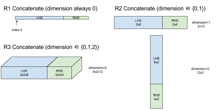
שרשור יוצר מערך מתוך אופרנדים מרובים של מערכים. המערך הוא באותו דירוג כמו כל אחד מהאופרנדים של מערך הקלט (שחייב להיות באותו דירוג כמו זה של זה) ומכיל את הארגומנטים לפי הסדר שבו הם צוינו.
Concatenate(operands..., dimension)
| ארגומנטים | סוג | סמנטיקה |
|---|---|---|
operands |
רצף של N XlaOp |
N מערכים מסוג T במידות [L0, L1, ...]. נדרש N >= 1. |
dimension |
int64 |
ערך במרווח [0, N) שמגדיר את המאפיין שיש לשרשר בין operands. |
למעט dimension, כל המאפיינים חייבים להיות זהים. הסיבה לכך היא שמערכת XLA לא תומכת במערכים "מסולסלים". כמו כן, שימו לב שאי אפשר לשרשר בין ערכי דירוג 0 (כי אי אפשר לתת שם למאפיין שבו מתרחשת השרשור).
דוגמה חד-ממדית:
Concat({ {2, 3}, {4, 5}, {6, 7} }, 0)
>>> {2, 3, 4, 5, 6, 7}
דוגמה דו-ממדית:
let a = {
{1, 2},
{3, 4},
{5, 6},
};
let b = {
{7, 8},
};
Concat({a, b}, 0)
>>> {
{1, 2},
{3, 4},
{5, 6},
{7, 8},
}
תרשים:
משפטי תנאי
למידע נוסף: XlaBuilder::Conditional.
Conditional(pred, true_operand, true_computation, false_operand,
false_computation)
| ארגומנטים | סוג | סמנטיקה |
|---|---|---|
pred |
XlaOp |
סולם מסוג PRED |
true_operand |
XlaOp |
ארגומנט מסוג \(T_0\) |
true_computation |
XlaComputation |
XlaComputation מסוג \(T_0 \to S\) |
false_operand |
XlaOp |
ארגומנט מסוג \(T_1\) |
false_computation |
XlaComputation |
XlaComputation מסוג \(T_1 \to S\) |
מבצעת true_computation אם pred היא true, false_computation אם pred
היא false ומחזירה את התוצאה.
השדה true_computation חייב לכלול ארגומנט אחד מסוג \(T_0\) , והוא יופעל עם true_operand שחייב להיות מאותו סוג. השדה false_computation חייב להכיל ארגומנט אחד מסוג \(T_1\) , והוא יופעל עם false_operand שחייב להיות מאותו סוג. סוג הערך
שמוחזר מ-true_computation ומ-false_computation חייב להיות זהה.
הערה: רק אחד מתוך true_computation ו-false_computation יופעל, בהתאם לערך של pred.
Conditional(branch_index, branch_computations, branch_operands)
| ארגומנטים | סוג | סמנטיקה |
|---|---|---|
branch_index |
XlaOp |
סולם מסוג S32 |
branch_computations |
רצף של N XlaComputation |
XlaComputations מסוג \(T_0 \to S , T_1 \to S , ..., T_{N-1} \to S\) |
branch_operands |
רצף של N XlaOp |
ארגומנטים מסוג \(T_0 , T_1 , ..., T_{N-1}\) |
מבצעת branch_computations[branch_index] ומחזירה את התוצאה. אם
branch_index הוא S32 שהוא < 0 או >= N, אז branch_computations[N-1] מופעל בתור הסתעפות ברירת המחדל.
כל branch_computations[b] חייב לכלול ארגומנט אחד מסוג \(T_b\) , והוא יופעל עם branch_operands[b] שחייב להיות מאותו סוג. סוג הערך המוחזר של כל branch_computations[b] חייב להיות זהה.
שימו לב שרק אחד מהערכים של branch_computations יתבצע בהתאם לערך של branch_index.
המרה (קונבולוציה)
למידע נוסף: XlaBuilder::Conv.
בתור ConvWithGeneralPadding, אבל המרווח הפנימי מצוין באופן קצר כ-SAME או valid. מרווח פנימי זהה ממיר את הקלט (lhs) באפסים, כך שהפלט יהיה זהה לצורה של הקלט כשלא נכנסים לחשבון. מרווח פנימי חוקי פירושו שאין מרווח פנימי.
ConvWithGeneralPadding (convolution)
למידע נוסף: XlaBuilder::ConvWithGeneralPadding.
מחשבת קונבולציה מהסוג שבו משתמשים ברשתות נוירונים. כאן אפשר לחשוב על קונבולציה כחלון לא-ממדי שנע על פני אזור בסיס N-ממדי, ומבוצע חישוב לכל מיקום אפשרי של החלון.
| ארגומנטים | סוג | סמנטיקה |
|---|---|---|
lhs |
XlaOp |
דירוג n+2 מערך קלטים |
rhs |
XlaOp |
דירוג n+2 מערך של משקלי ליבה |
window_strides |
ArraySlice<int64> |
מערך n-d של צעדים בליבה |
padding |
ArraySlice< pair<int64,int64>> |
מערך n-d של מרווח פנימי (נמוך, גבוה) |
lhs_dilation |
ArraySlice<int64> |
מערך גורמי הרחבה מסוג n-d lhs |
rhs_dilation |
ArraySlice<int64> |
מערך גורמי הרחבה מסוג n-d rhs |
feature_group_count |
int64 | מספר הקבוצות של התכונות |
batch_group_count |
int64 | המספר של קבוצות אצווה |
תהי n של מספר המימדים המרחביים. הארגומנט lhs הוא מערך בדירוג n+2 שמתאר את אזור הבסיס. זה נקרא הקלט, למרות שכמובן גם
ה-rhs הוא קלט. ברשת נוירונים, אלה הפעלות הקלט.
מאפייני n+2 הם, בסדר הבא:
batch: כל קואורדינטה במאפיין הזה מייצגת קלט עצמאי שעבורו מתבצעת קונבולציה.z/depth/features: לכל מיקום (y,x) באזור הבסיס משויך וקטור שנוסף למאפיין הזה.spatial_dims: מתאר אתnהמימדים המרחביים שמגדירים את אזור הבסיס שבו החלון נע.
הארגומנט rhs הוא מערך דירוג n+2 שמתאר את המסנן/הליבה (kernel)/החלון המתקפל. המאפיינים הם, בסדר הבא:
output-z: המאפייןzשל הפלט.input-z: גודל המימד הזה כפולfeature_group_countצריך להיות שווה לגודל של המאפייןzבשניות.spatial_dims: מתאר אתnהמימדים המרחביים שמגדירים את חלון ה-n-d שנע על פני אזור הבסיס.
הארגומנט window_strides מציין את הרוחב של החלון הקונבולוציה במימדים המרחביים. לדוגמה, אם הצלעה במאפיין המרחבי הראשון היא 3, אז ניתן למקם את החלון רק בקואורדינטות שבהן האינדקס המרחבי הראשון מתחלק ב-3.
הארגומנט padding מציין את הכמות של אפס מרווח פנימי שיש להחיל על אזור הבסיס. מידת המרווח הפנימי יכולה להיות שלילית. הערך המוחלט של מרווח פנימי שלילי מציין את מספר הרכיבים שיש להסיר מהמאפיין שצוין לפני ביצוע הקונבולוציה. padding[0] מציין את המרווח הפנימי במאפיין y והרווח padding[1] מציין את המרווח הפנימי של המאפיין x. לכל צמד יש מרווח פנימי נמוך כרכיב הראשון, והמרווח הפנימי הגבוה הוא הרכיב השני. המרווח הפנימי הנמוך מוחל בכיוון של האינדקסים הנמוכים יותר, והמרווח הפנימי העליון מוחל בכיוון של האינדקסים הגבוהים יותר. לדוגמה, אם הערך של padding[1] הוא (2,3), יופיע מרווח של 2 אפסים בצד שמאל ו-3 אפסים בצד ימין במאפיין המרחבי השני. השימוש במרווח פנימי הוא שווה ערך להוספה של אותם ערכי אפס לקלט (lhs) לפני ביצוע הקונבולוציה.
הארגומנטים lhs_dilation ו-rhs_dilation מציינים את גורם ההרחבה שיש להחיל על rhs ו-rhs, בהתאמה, בכל ממד מרחבי. אם גורם ההרחבות של מימד מרחבי הוא d, אז חורי d-1 מוצבים באופן מרומז בין כל אחד מהערכים במימד הזה, ומגדילים את המערך. החורים ימולאו בערך 'no-op', שמשמעותו בקונבולוציה היא אפס.
התרחבות של ה-rhs נקראת גם 'קונבולציה מזעזעת'. למידע נוסף: tf.nn.atrous_conv2d. הרחבה של הליצים נקראת גם 'קונבולוציה הופכת'. לפרטים נוספים: tf.nn.conv2d_transpose.
אפשר להשתמש בארגומנט feature_group_count (ערך ברירת המחדל 1) כדי ליצור קונבולוציות מקובצות. feature_group_count צריך להיות מחלק גם של הקלט וגם של מאפיין תכונת הפלט. אם feature_group_count גדול מ-1, המשמעות היא שמושגי מימד תכונת הקלט והפלט ומאפיין תכונת הפלט rhs מתפצלים באופן שווה לקבוצות רבות של feature_group_count, כשכל קבוצה מכילה רצף משנה עוקב של תכונות. מימד תכונת הקלט של rhs צריך להיות שווה למאפיין של תכונת הקלט lhs חלקי feature_group_count (כך שכבר יש לו גודל של קבוצה של תכונות קלט). קבוצות i-th משמשות יחד כדי לחשב את feature_group_count לפונבולציות נפרדות רבות. התוצאות של התכוונונים האלה משורשרות יחד במאפיין תכונת הפלט.
כדי לבצע קונבולציה לעומק, הארגומנט feature_group_count יוגדר
למימד של תכונת הקלט, והמסנן יעוצב מחדש מ-[filter_height, filter_width, in_channels, channel_multiplier] ל-[filter_height, filter_width, 1, in_channels * channel_multiplier]. לפרטים נוספים: tf.nn.depthwise_conv2d.
אפשר להשתמש בארגומנט batch_group_count (ערך ברירת מחדל 1) למסננים
מקובצים במהלך הפצה לאחור. הערך batch_group_count צריך להיות מחלק
בגודל של מאפיין האצווה lhs (קלט). אם batch_group_count גדול מ-1, המשמעות היא שמאפיין קבוצת הפלט צריך להיות בגודל input batch
/ batch_group_count. הערך batch_group_count חייב להיות מחלק של גודל התכונה
של הפלט.
לצורת הפלט יש מימדים אלה, בסדר הבא:
batch: גודל המאפיין הזה כפולbatch_group_countצריך להיות שווה לגודל של המאפייןbatchבשניות.z: גודל זהה לזה שלoutput-zבליבה (rhs).spatial_dims: ערך אחד לכל מיקום חוקי של חלון הקונבולוציה.

האיור שלמעלה מציג את אופן הפעולה של השדה batch_group_count. בפועל, אנחנו מפצלים כל מערכי נתונים לקבוצות batch_group_count ועושים את אותו הדבר לגבי תכונות הפלט. לאחר מכן, עבור כל אחת מהקבוצות האלה, אנחנו מבצעים צמדים של קונבולציות (קונבולציות) ושרשורים את הפלט לאורך מאפיין תכונת הפלט. הסמנטיקה התפעולית של כל שאר המאפיינים (תכונה ומרחב) נשארת ללא שינוי.
המיקומים החוקיים של החלון הקונבולוציה נקבעים לפי הצעדים וגודל שטח הבסיס אחרי המרווח הפנימי.
כדי לתאר מה עושה קונבולציה, כדאי לחשוב על קונבולציה דו-ממדית ולבחור בפלט כמה קואורדינטות קבועות של batch, z, y, x. לאחר מכן, (y,x) הוא המיקום של פינת החלון בתוך אזור הבסיס (למשל, הפינה השמאלית העליונה, בהתאם לאופן שבו אתם מפרשים את המימדים המרחביים). עכשיו יש לנו חלון דו-ממדי שנלקח מאזור הבסיס, שבו כל נקודה דו-ממדית משויכת לווקטור חד-ממדי, ולכן יש לנו תיבה בתלת-ממד. מהליבה המסתובלת, מאז שתיקנו את
קואורדינטת הפלט z, יש לנו גם תיבה בתלת-ממד. לשתי התיבות יש אותם מימדים, כך שנוכל לקחת את סכום המוצרים ברמת הרכיבים בשתי התיבות (בדומה למכפלה סקלרית). זהו ערך הפלט.
שימו לב שאם output-z הוא למשל, 5, כל מיקום של החלון מייצר 5 ערכים בפלט אל המאפיין z של הפלט. הערכים האלה שונים בחלק של הליבה המתפתל שבו נעשה שימוש – לכל קואורדינטת output-z יש תיבה נפרדת בתלת-ממד של ערכים. אפשר לחשוב על זה בתור 5
קונבולוציות נפרדות עם מסנן שונה לכל אחת מהן.
לפניכם קוד פסאודו-קוד ליצירת קונבולציה דו-ממדית עם מרווח פנימי וצעדים:
for (b, oz, oy, ox) {  // output coordinates
  value = 0;
  for (iz, ky, kx) {  // kernel coordinates and input z
    iy = oy*stride_y + ky - pad_low_y;
    ix = ox*stride_x + kx - pad_low_x;
    if ((iy, ix) inside the base area considered without padding) {
      value += input(b, iz, iy, ix) * kernel(oz, iz, ky, kx);
    }
  }
  output(b, oz, oy, ox) = value;
}
ConvertElementType
למידע נוסף: XlaBuilder::ConvertElementType.
בדומה לפעולת ההמרה static_cast שכוללת רכיבים ב-C++, היא מבצעת פעולת המרה
מבחינת רכיבים מצורת נתונים לצורת יעד. המאפיינים חייבים
להיות תואמים, וההמרה היא רכיב ברכיב. למשל, רכיבי s32 הופכים לרכיבי
f32 באמצעות תרחיש המרה מ-s32 ל-f32.
ConvertElementType(operand, new_element_type)
| ארגומנטים | סוג | סמנטיקה |
|---|---|---|
operand |
XlaOp |
מערך מסוג T עם עמעום D |
new_element_type |
PrimitiveType |
סוג U |
מידות האופרנד וצורת היעד חייבות להתאים. אסור שיהיו פיצולים בין סוגי רכיבי המקור ורכיב היעד.
המרה כמו T=s32 ל-U=f32 תבצע תרחיש של המרות מסוג 'מספר שלם', למשל 'מסביב עד זוגי'.
let a: s32[3] = {0, 1, 2};
let b: f32[3] = convert(a, f32);
then b == f32[3]{0.0, 1.0, 2.0}
CrossReplicaSum
מבצעת AllReduce עם חישוב של סכום.
CustomCall
למידע נוסף: XlaBuilder::CustomCall.
הפעלה של פונקציה שסופקה על ידי משתמש בתוך חישוב.
CustomCall(target_name, args..., shape)
| ארגומנטים | סוג | סמנטיקה |
|---|---|---|
target_name |
string |
שם הפונקציה. תושמע הוראה לשיחה שמתמקדת בשם הסמל הזה. |
args |
רצף של N XlaOp שנ' |
N ארגומנטים מסוג שרירותי, שיועברו לפונקציה. |
shape |
Shape |
צורת הפלט של הפונקציה |
חתימת הפונקציה זהה, ללא קשר לארגומנטים או לסוג הארגומנטים:
extern "C" void target_name(void* out, void** in);
לדוגמה, אם נעשה שימוש ב-CustomCall באופן הבא:
let x = f32[2] {1,2};
let y = f32[2x3] { {10, 20, 30}, {40, 50, 60} };

CustomCall("myfunc", {x, y}, f32[3x3])
הנה דוגמה להטמעה של myfunc:
extern "C" void myfunc(void* out, void** in) {
  float (&x)[2] = *static_cast<float(*)[2]>(in[0]);
  float (&y)[2][3] = *static_cast<float(*)[2][3]>(in[1]);
  EXPECT_EQ(1, x[0]);
  EXPECT_EQ(2, x[1]);
  EXPECT_EQ(10, y[0][0]);
  EXPECT_EQ(20, y[0][1]);
  EXPECT_EQ(30, y[0][2]);
  EXPECT_EQ(40, y[1][0]);
  EXPECT_EQ(50, y[1][1]);
  EXPECT_EQ(60, y[1][2]);
  float (&z)[3][3] = *static_cast<float(*)[3][3]>(out);
  z[0][0] = x[1] + y[1][0];
  // ...
}
לפונקציה שסופקה על ידי המשתמש אסור שיהיו תופעות לוואי, וההפעלה שלה חייבת להיות זהה.
נקודה
למידע נוסף: XlaBuilder::Dot.
Dot(lhs, rhs)
| ארגומנטים | סוג | סמנטיקה |
|---|---|---|
lhs |
XlaOp |
מערך מסוג T |
rhs |
XlaOp |
מערך מסוג T |
הסמנטיקה המדויקת של פעולה זו תלויה בדירוג האופרנדים:
| קלט | פלט | סמנטיקה |
|---|---|---|
וקטור [n] dot וקטור [n] |
סקלרי | מכפלה וקטורית נקודה |
מטריצה [m x k] dot וקטור [k] |
וקטור [m] | הכפלת מטריצה-וקטורית |
מטריצה [m x k] מטריצה של dot [k x n] |
מטריצה [m x n] | הכפלת מטריצות |
הפעולה מבצעת סכום של מוצרים במאפיין השני של lhs (או הראשון אם יש לו דירוג 1) והמאפיין הראשון של rhs. אלו המאפיינים ה"מכווצים". המידות שמוסכמים בחוזה של lhs ו-rhs חייבות להיות באותו גודל. בפועל, אפשר להשתמש בה כדי לבצע מכפלות נקודות בין וקטורים, הכפלות וקטורים/מטריצה או הכפלות של מטריצות/מטריצה.
DotGeneral
למידע נוסף: XlaBuilder::DotGeneral.
DotGeneral(lhs, rhs, dimension_numbers)
| ארגומנטים | סוג | סמנטיקה |
|---|---|---|
lhs |
XlaOp |
מערך מסוג T |
rhs |
XlaOp |
מערך מסוג T |
dimension_numbers |
DotDimensionNumbers |
מספרים לכיווץ ולמספר מידות באצווה |
דומה ל-Dot, אך מאפשר לציין מספרי מימדים של אצווה וחוזים גם ב-lhs וגם ב-rhs.
| שדות DotdimensionNumbers | סוג | סמנטיקה |
|---|---|---|
lhs_contracting_dimensions
|
int64 חוזר | lhs מספרים של מאפיינים
חוזיים |
rhs_contracting_dimensions
|
int64 חוזר | rhs מספרים של מאפיינים
חוזיים |
lhs_batch_dimensions
|
int64 חוזר | מספרים של lhs מידות
|
rhs_batch_dimensions
|
int64 חוזר | מספרים של rhs מידות
|
DotGeneral מבצעת את סכום המוצרים בהתאם למידות החוזה שצוינו ב-dimension_numbers.
מספרי המאפיינים הקשורים בחוזה מ-lhs ומ-rhs לא חייבים להיות זהים, אבל מידות המידות שלהם צריכות להיות זהות.
דוגמה למספרים של מאפיינים חוזיים:
lhs = { {1.0, 2.0, 3.0},
{4.0, 5.0, 6.0} }

rhs = { {1.0, 1.0, 1.0},
{2.0, 2.0, 2.0} }

DotDimensionNumbers dnums;
dnums.add_lhs_contracting_dimensions(1);
dnums.add_rhs_contracting_dimensions(1);

DotGeneral(lhs, rhs, dnums) -> { {6.0, 12.0},
{15.0, 30.0} }
למספרים של מאפייני אצווה משויכים מ-lhs ומ-rhs חייבים להיות אותם מידות.
דוגמה למספרי מידות באצווה (גודל אצווה 2, מטריצות 2x2):
lhs = { { {1.0, 2.0},
{3.0, 4.0} },
{ {5.0, 6.0},
{7.0, 8.0} } }

rhs = { { {1.0, 0.0},
{0.0, 1.0} },
{ {1.0, 0.0},
{0.0, 1.0} } }

DotDimensionNumbers dnums;
dnums.add_lhs_contracting_dimensions(2);
dnums.add_rhs_contracting_dimensions(1);
dnums.add_lhs_batch_dimensions(0);
dnums.add_rhs_batch_dimensions(0);

DotGeneral(lhs, rhs, dnums) -> { { {1.0, 2.0},
{3.0, 4.0} },
{ {5.0, 6.0},
{7.0, 8.0} } }
| קלט | פלט | סמנטיקה |
|---|---|---|
[b0, m, k] dot [b0, k, n] |
[b0, m, n] | אצווה מאטמול |
[b0, b1, m, k] dot [b0, b1, k, n] |
[b0, b1, m, n] | אצווה מאטמול |
לאחר מכן מספר המאפיין שמתקבל מתחיל במאפיין האצווה, לאחר מכן במאפיין lhs שאינו מקוצר/לא באצווה, ולבסוף במאפיין rhs שאינו מתכווץ/לא באצווה.
DynamicSlice
למידע נוסף: XlaBuilder::DynamicSlice.
DynamicSlice מחלץ מערך משנה ממערך הקלט ב-start_indices הדינמי. גודל הפלח בכל מאפיין מועבר באמצעות size_indices, שמציין את נקודת הסיום של מרווחי הפרוסות הבלעדיים בכל מאפיין: [התחלה, התחלה + גודל). הצורה של start_indices חייבת להיות דירוג == 1, כאשר גודל המאפיין שווה לדירוג operand.
DynamicSlice(operand, start_indices, size_indices)
| ארגומנטים | סוג | סמנטיקה |
|---|---|---|
operand |
XlaOp |
מערך ממדי N מסוג T |
start_indices |
רצף של N XlaOp |
רשימה של N מספרים שלמים סקלרים המכילים את האינדקסים המתחילים של הפלח עבור כל מימד. הערך חייב להיות גדול מ-0 או שווה לו. |
size_indices |
ArraySlice<int64> |
רשימה של N מספרים שלמים שמכילה את גודל הפלח לכל מאפיין. כל ערך חייב להיות גדול מאפס, וגודל התחלה + גודל חייב להיות קטן מגודל המאפיין או שווה לו, כדי להימנע מגלישת גודל של מאפיין מודולו. |
המדד של הפלחים האפקטיביים מחושבים על ידי החלת הטרנספורמציה הבאה על כל אינדקס i ב-[1, N) לפני ביצוע הפלח:
start_indices[i] = clamp(start_indices[i], 0, operand.dimension_size[i] - size_indices[i])
כך אפשר להבטיח שהפרוסה שחולצת תהיה תמיד בגבולות ביחס למערך האופרנד. אם הפלח נמצא בגבולות לפני החלת הטרנספורמציה, לטרנספורמציה אין השפעה.
דוגמה חד-ממדית:
let a = {0.0, 1.0, 2.0, 3.0, 4.0}
let s = {2}

DynamicSlice(a, s, {2}) produces:
{2.0, 3.0}
דוגמה דו-ממדית:
let b =
{ {0.0,  1.0,  2.0},
{3.0,  4.0,  5.0},
{6.0,  7.0,  8.0},
{9.0, 10.0, 11.0} }
let s = {2, 1}

DynamicSlice(b, s, {2, 2}) produces:
{ { 7.0,  8.0},
{10.0, 11.0} }
DynamicUpdateSlice
למידע נוסף: XlaBuilder::DynamicUpdateSlice.
DynamicUpdateSlice יוצר תוצאה שהיא הערך של מערך הקלט operand, כאשר פרוסה update מוחלפת ב-start_indices.
הצורה של update קובעת את הצורה של מערך המשנה של התוצאה שתעודכן.
הצורה של start_indices חייבת להיות דירוג == 1, כאשר גודל המאפיין שווה לדירוג operand.
DynamicUpdateSlice(operand, update, start_indices)
| ארגומנטים | סוג | סמנטיקה |
|---|---|---|
operand |
XlaOp |
מערך ממדי N מסוג T |
update |
XlaOp |
מערך ממדי N מסוג T שמכיל את עדכון הפלח. כל מימד בצורת עדכון חייב להיות גדול מאפס, וכל מאפיין 'התחלת + עדכון' חייב להיות קטן מגודל האופרנד או שווה לו עבור כל מאפיין, כדי להימנע מיצירת אינדקסים של עדכון מחוץ לתחום. |
start_indices |
רצף של N XlaOp |
רשימה של N מספרים שלמים סקלרים המכילים את האינדקסים המתחילים של הפלח עבור כל מימד. הערך חייב להיות גדול מ-0 או שווה לו. |
המדד של הפלחים האפקטיביים מחושבים על ידי החלת הטרנספורמציה הבאה על כל אינדקס i ב-[1, N) לפני ביצוע הפלח:
start_indices[i] = clamp(start_indices[i], 0, operand.dimension_size[i] - update.dimension_size[i])
כך אפשר להבטיח שהפרוסה המעודכנת תהיה תמיד בגבולות ביחס למערך האופרנד. אם הפלח נמצא בגבולות לפני החלת הטרנספורמציה, לטרנספורמציה אין השפעה.
דוגמה חד-ממדית:
let a = {0.0, 1.0, 2.0, 3.0, 4.0}
let u = {5.0, 6.0}
let s = {2}

DynamicUpdateSlice(a, u, s) produces:
{0.0, 1.0, 5.0, 6.0, 4.0}
דוגמה דו-ממדית:
let b =
{ {0.0,  1.0,  2.0},
{3.0,  4.0,  5.0},
{6.0,  7.0,  8.0},
{9.0, 10.0, 11.0} }
let u =
{ {12.0,  13.0},
{14.0,  15.0},
{16.0,  17.0} }

let s = {1, 1}

DynamicUpdateSlice(b, u, s) produces:
{ {0.0,  1.0,  2.0},
{3.0, 12.0, 13.0},
{6.0, 14.0, 15.0},
{9.0, 16.0, 17.0} }
פעולות חשבון בינאריות עם רכיבים
למידע נוסף: XlaBuilder::Add.
יש תמיכה בקבוצה של פעולות אריתמטיות בינאריות ברמת הרכיב.
Op(lhs, rhs)
כאשר Op הוא אחד מהערכים Add (חיבור), Sub (חיסור), Mul (כפל), Div (חילוק), Rem (יתרה), Max (מקסימום), Min (מינימום), LogicalAnd (וגם לוגי) או LogicalOr (OR לוגי).
| ארגומנטים | סוג | סמנטיקה |
|---|---|---|
lhs |
XlaOp |
אופרנד צד שמאל: מערך מסוג T |
rhs |
XlaOp |
אופרנד צד ימין: מערך מסוג T |
הצורות של הארגומנטים צריכות להיות דומות או תואמות. במסמכי התיעוד בנושא שידור מוסבר מה המשמעות של תאימות של צורות. לתוצאה של פעולה יש צורה שהיא התוצאה של שידור שני מערכי הקלט. בווריאנט הזה, אין תמיכה בפעולות בין מערכים של דרגות שונות, אלא אם אחד מהאופרנדים הוא סקלרי.
כשהערך של Op הוא Rem, הסימן של התוצאה נלקח מהדיבידנד, והערך המוחלט של התוצאה תמיד קטן מהערך המוחלט של המחלק.
גלישת חלוקה של מספרים שלמים (חלוקה חתומה/לא חתומה/נשארת באפס או חלוקה
חתומה/שארית INT_SMIN עם -1) יוצרת ערך מוגדר
להטמעה.
קיימת וריאציה חלופית עם תמיכה בשידור ברמות שונות לפעולות האלה:
Op(lhs, rhs, broadcast_dimensions)
כאשר Op זהה למעלה. כדאי להשתמש בווריאנט הזה של הפעולה לביצוע פעולות אריתמטיות בין מערכים בעלי דרגות שונות (למשל, הוספת מטריצה לווקטור).
האופרנד הנוסף broadcast_dimensions הוא קטע של מספרים שלמים שמשמש להרחבת הדירוג של אופרנד מהדירוג הנמוך יותר עד לדירוג של אופרנד
מהדירוג הגבוה יותר. broadcast_dimensions ממפה את ממדי הצורה בעלת הדירוג הנמוך למידות של הצורה בעלת הדירוג הגבוה יותר. הממדים הלא ממופים של הצורה המורחבת מלאים במידות בגודל 1. שידור של מימדים מצומצמים משדר את הצורות לאורך הממדים המנוונים האלה, כדי להשוות את הצורות של שני האופרנדים. הסמנטיקה מתוארת בפירוט בדף השידור.
פעולות השוואה ברמת הרכיב
למידע נוסף: XlaBuilder::Eq.
יש תמיכה בקבוצה של פעולות סטנדרטיות להשוואה בינאריות עם רכיב. שימו לב שהסמנטיקה הרגילה של השוואה בין נקודות צפות ב-IEEE 754 חלה כשמשווים בין סוגים של נקודות צפות.
Op(lhs, rhs)
כאשר Op הוא אחד מהערכים Eq (שווה ל-), Ne (לא שווה ל-), Ge
(גדול או שווה מ-), Gt (גדול מ-), Le (פחות או שווה ל-), Lt
(פחות מ-). קבוצה אחרת של אופרטורים, EqTotalOrder, NeTotalOrder, GeTotalOrder, GtTotalOrder, LeTotalOrder ו-LtTotalOrder, שמאובטחת אותן פונקציות, מספקת את אותן הפונקציות, מלבד העובדה שהם תומכים בהזמנות כוללות מעל מספרי הנקודות הצפה, על ידי אכיפה של -NaN < -Inf < -Finite < -0 < +N +Na
| ארגומנטים | סוג | סמנטיקה |
|---|---|---|
lhs |
XlaOp |
אופרנד צד שמאל: מערך מסוג T |
rhs |
XlaOp |
אופרנד צד ימין: מערך מסוג T |
הצורות של הארגומנטים צריכות להיות דומות או תואמות. במסמכי התיעוד בנושא שידור מוסבר מה המשמעות של תאימות של צורות. לתוצאה של פעולה יש צורה שהיא התוצאה של שידור שני מערכי הקלט עם סוג הרכיב PRED. בווריאנט הזה, אין תמיכה בפעולות בין מערכים בדרגות שונות, אלא אם אחד מהאופרנדים הוא סקלרי.
קיימת וריאציה חלופית עם תמיכה בשידור ברמות שונות לפעולות האלה:
Op(lhs, rhs, broadcast_dimensions)
כאשר Op זהה למעלה. כדאי להשתמש בווריאנט של הפעולה לביצוע פעולות השוואה בין מערכים בדרגות שונות (למשל, הוספת מטריצה לווקטור).
האופרנד הנוסף broadcast_dimensions הוא פלח של מספרים שלמים, שמציין את המימדים שישמשו לשידור האופרנדים. הסמנטיקה מתוארת בפירוט בדף השידור.
פונקציות אונריות עם רכיבים
ב-XlaBuilder יש תמיכה בפונקציות אונריות הבאות עם הרכיבים:
Abs(operand) AB מבוסס-רכיבים x -> |x|.
Ceil(operand) גובה הרכיב x -> ⌈x⌉.
Cos(operand) קוסינוס x -> cos(x) ברמת הרכיב.
Exp(operand) מעריכי טבעי x -> e^x ברמת הרכיב.
Floor(operand) קומה x -> ⌊x⌋ ברמת הרכיב.
Imag(operand) החלק המדומה ברמת הרכיב של צורה מורכבת (או אמיתית). x -> imag(x). אם האופרנד הוא סוג של נקודה צפה (floating-point), הפונקציה מחזירה את הערך 0.
IsFinite(operand) בודקת אם כל רכיב של operand הוא סופי, כלומר אינו אינסוף חיובי או שלילי ואינו NaN. מחזירה מערך של ערכי PRED עם אותה צורה כמו הקלט, כאשר כל רכיב הוא true רק אם רכיב הקלט המתאים הוא סופי.
Log(operand) לוגריתם טבעי x -> ln(x) ברמת הרכיב.
LogicalNot(operand) לוגיקת רכיב ולא x -> !(x).
Logistic(operand) חישוב של פונקציה לוגיסטית ברמת הרכיב x ->
logistic(x).
PopulationCount(operand) מחשבת את מספר הביטים שמוגדרים בכל רכיב של operand.
Neg(operand) שלילה ברמת הרכיב x -> -x.
Real(operand), מבחינת הרכיב, החלק האמיתי של צורה מורכבת (או ממשית).
x -> real(x). אם האופרנד הוא סוג של נקודה צפה (floating-point), מחזירה את אותו ערך.
Rsqrt(operand) הדדית ברמת הרכיב של פעולת שורש ריבועית
x -> 1.0 / sqrt(x).
Sign(operand) פעולת סימן ברכיב x -> sgn(x) כאשר
\[\text{sgn}(x) = \begin{cases} -1 & x < 0\\ -0 & x = -0\\ NaN & x = NaN\\ +0 & x = +0\\ 1 & x > 0 \end{cases}\]
באמצעות אופרטור ההשוואה של סוג הרכיב operand.
Sqrt(operand) פעולת שורש ריבועית ברמת הרכיב x -> sqrt(x).
Cbrt(operand) פעולת שורש מעוקב ברמת רכיב x -> cbrt(x).
Tanh(operand) טנגנס היפרבולי ברמת הרכיב x -> tanh(x).
Round(operand) עיגול יסודות, במרחק קשר מאפס.
RoundNearestEven(operand) עיגול ברמת הרכיב, לקישור הזוגי הקרוב ביותר.
| ארגומנטים | סוג | סמנטיקה |
|---|---|---|
operand |
XlaOp |
האופרנד לפונקציה |
הפונקציה מוחלת על כל רכיב במערך operand, וכתוצאה מכך נוצר מערך עם אותה צורה. operand יכול להיות סקלרי (דירוג 0).
Fft
הפעולה XLA FFT מטמיעה את התמרות פורייה (הטרנספורמציה של פורייה) קדימה והפוכה, בקלט ובפלט אמיתיים ומורכבים. יש תמיכה ב-FFT רב-מימדי עם עד 3 צירים.
למידע נוסף: XlaBuilder::Fft.
| ארגומנטים | סוג | סמנטיקה |
|---|---|---|
operand |
XlaOp |
המערך שאנחנו ממירים באמצעות פורייה. |
fft_type |
FftType |
פרטים נוספים מפורטים בטבלה שבהמשך. |
fft_length |
ArraySlice<int64> |
אורכי דומיין הזמן של הצירים שמשתנים. הפעולה הזו נדרשת באופן ספציפי כדי ש-IRFFT יגודל ישר של הציר הפנימי ביותר, כי ל-RFFT(fft_length=[16]) יש צורת פלט זהה לזו של RFFT(fft_length=[17]). |
FftType |
סמנטיקה |
|---|---|
FFT |
העברה של FFT מורכב למורכב. הצורה לא השתנתה. |
IFFT |
פונקציית ה-FFT הפוכה, מורכבת למורכב, הצורה לא השתנתה. |
RFFT |
העברה של FFT אמתי למורכב. צורת הציר הפנימי ביותר מצטמצמת ל-fft_length[-1] // 2 + 1 אם fft_length[-1] הוא ערך שאינו אפס, ללא החלק המצומד ההפוך של האות שהשתנה מעבר לתדר Nyquist. |
IRFFT |
FFT ההופכי מריאל למורכב (כלומר, לוקח מורכב, מוחזרת בפועל). צורת הציר הפנימי ביותר מורחבת ל-fft_length[-1] אם fft_length[-1] הוא ערך שאינו אפס, ומסיקים את החלק של האות שהשתנה מעבר לתדר ה-Nyquist מהצימוד ההפוך של הערכים 1 ל-fft_length[-1] // 2 + 1. |
הרשאות בסיסיות (FFT) רב-ממדי
אם מספקים יותר מ-fft_length אחד, הפעולה הזו מקבילה להחלת סדרת פעולות FFT על כל אחד מהצירים הפנימיים ביותר. שימו לב שבמקרים אמיתיים->מורכבים->מורכבים->מציאות, הטרנספורמציה של הציר הפנימי ביותר (בפועל) מבוצעת קודם (RFFT, אחרון ל-IRFFT), ולכן הציר הפנימי הוא זה שמשנה את הגודל. לאחר מכן טרנספורמציות צירים אחרות יהיו
מורכבות->מורכבות.
פרטי ההטמעה
ה-CPU FFT מגובה על ידי TensorFFT של Eigen. ב-GPU FFT נעשה שימוש ב-cuFFT.
איסוף
הפעולה של XLA אוספת ביחד כמה פרוסות (כל פרוסה במרווח זמן ריצה שונה, שעשוי להיות שונה) של מערך קלט.
סמנטיקה כללית
למידע נוסף: XlaBuilder::Gather.
לתיאור אינטואיטיבי יותר, ניתן לעיין בקטע "תיאור לא רשמי" בהמשך.
gather(operand, start_indices, offset_dims, collapsed_slice_dims, slice_sizes, start_index_map)
| ארגומנטים | סוג | סמנטיקה |
|---|---|---|
operand |
XlaOp |
המערך שאנחנו אוספים. |
start_indices |
XlaOp |
מערך שמכיל את האינדקסים הראשונים של הפרוסות שאנחנו אוספים. |
index_vector_dim |
int64 |
המאפיין בstart_indices ש "מכיל" את האינדקסים הראשונים. בהמשך מופיע תיאור מפורט. |
offset_dims |
ArraySlice<int64> |
קבוצת המימדים בצורת הפלט שמשתלבים למערך שמפולח מאופרנד. |
slice_sizes |
ArraySlice<int64> |
slice_sizes[i] הוא הגבול של הפלח במאפיין i. |
collapsed_slice_dims |
ArraySlice<int64> |
קבוצת המימדים בכל פרוסה שמוצגת במצב כיווץ. המאפיינים האלה צריכים להיות בגודל 1. |
start_index_map |
ArraySlice<int64> |
מפה שמתארת איך למפות אינדקסים בstart_indices לאינדקסים משפטיים בתוך אופרנד. |
indices_are_sorted |
bool |
האם מובטחת שהאינדקסים ימוינו על ידי מבצע הקריאה. |
unique_indices |
bool |
האם מובטחת שהאינדקסים יהיו ייחודיים על ידי מבצע הקריאה. |
לשם נוחות, אנחנו מסמנים מאפיינים במערך הפלט שאינם ב-offset_dims כ-batch_dims.
הפלט הוא מערך של דרגות batch_dims.size + offset_dims.size.
הערך operand.rank חייב להיות שווה לסכום של offset_dims.size ו-collapsed_slice_dims.size. בנוסף, slice_sizes.size צריך להיות שווה ל-operand.rank.
אם index_vector_dim שווה ל-start_indices.rank, אנחנו מתייחסים באופן לא מפורש
ל-start_indices למאפיין 1 בסוף (כלומר אם start_indices היה
שהצורה [6,7] ו-index_vector_dim הוא 2, אנחנו מחשיבים באופן לא מפורש
שהצורה של start_indices כ-[6,7,1]).
הגבולות של מערך הפלט לאורך המאפיין i מחושבים באופן הבא:
אם המאפיין
iמופיע ב-batch_dims(כלומר, שווה ל-batch_dims[k]בערךk), אנחנו בוחרים את המאפיין המתאים מתוךstart_indices.shape, ומדלגים עלindex_vector_dim(כלומר, בוחרים באפשרותstart_indices.shape.dims[k] אםk<index_vector_dimוגםstart_indices.shape.dims[k+1]).אם
iקיים בoffset_dims(כלומר שווה ל-offset_dims[k] בערךk), אנחנו בוחרים את הגבול התואם שלslice_sizesאחריcollapsed_slice_dims(כלומר, אנחנו בוחריםadjusted_slice_sizes[k], כאשרadjusted_slice_sizesהואslice_sizesומסירים את הגבולות מהמדדיםcollapsed_slice_dims).
באופן רשמי, אינדקס האופרנד In שתואם לאינדקס הפלט הנתון Out מחושב באופן הבא:
הפונקציה
G= {Out[k] עבורkב-batch_dims}. אפשר להשתמש ב-Gכדי לחתוך את וקטורSכך ש-S[i] =start_indices[שילוב(G,i)] כאשר שילוב(A, b) יוסיף את b במיקוםindex_vector_dimל-A. שימו לב שההגדרה הזו מוגדרת היטב גם אםGריק: אם השדהGריק, אזS=start_indices.יוצרים אינדקס התחלתי,
Sin, אלoperandבאמצעותSעל ידי פיזורSבאמצעותstart_index_map. ליתר דיוק:Sin[start_index_map[k]] =S[k] אםk<start_index_map.size.Sin[_] =0אחרת.
אפשר ליצור אינדקס
Oinבתוךoperandעל ידי פיזור האינדקסים במאפייני ההיסט ב-Outלפי הקבוצהcollapsed_slice_dims. ליתר דיוק:Oin[remapped_offset_dims(k)] =Out[offset_dims[k]] אםk<offset_dims.size(remapped_offset_dimsמוגדר למטה).Oin[_] =0אחרת.
InהואOin+Sin, כאשר + הוא תוספת רכיב.
remapped_offset_dims היא פונקציה מונוטונית עם הדומיין [0,
offset_dims.size) והטווח [0, operand.rank) \ collapsed_slice_dims. לכן, אם, offset_dims.size הוא 4, operand.rank הוא 6
collapsed_slice_dims הוא {0, 2} ואז remapped_offset_dims הוא {0←1,
1←3, 2←4, 3←5}.
אם המדיניות indices_are_sorted מוגדרת כ-True, אז XLA יכולה להניח ש-start_indices ממוינים (בסדר start_index_map עולה) על ידי המשתמש. אם הם לא תואמים, אז יש בסמנטיקה של הטמעה כזו.
אם המדיניות unique_indices מוגדרת כ-True, המערכת של XLA יכולה להניח שכל הרכיבים
שמפוזרים עד הם ייחודיים. XLA יכולה להשתמש בפעולות לא אטומיות. אם
unique_indices מוגדר כ-True והאינדקסים שמפוזרים אליהם לא
ייחודיים, מוגדרת הטמעה של הסמנטיקה.
תיאור ודוגמאות פשוטים
באופן לא רשמי, כל אינדקס Out במערך הפלט תואם לרכיב E במערך האופרנד, והוא מחושב באופן הבא:
אנחנו משתמשים במאפייני האצווה ב-
Outכדי לחפש אינדקס פתיחה מ-start_indices.אנחנו משתמשים ב-
start_index_mapכדי למפות את האינדקס ההתחלתי (שהגודל שלו עשוי להיות קטן מ-operand.rank) לאינדקס התחלתי 'מלא' לתוךoperand.אנחנו פורסים פרוסה דינמית בגודל
slice_sizesעל סמך אינדקס הפתיחה המלא.אנחנו מעצבים מחדש את הפלח על ידי כיווץ המידות של
collapsed_slice_dims. מאחר שכל המידות של הפלחים המכווצים חייבים להיות מוגבלים ל-1, הצורה מחדש תמיד חוקית.אנחנו משתמשים במאפייני ההיסט ב-
Outכדי ליצור אינדקס לפרוסה הזו, וכך לקבל את רכיב הקלטE, שתואם לאינדקס הפלטOut.
הערך index_vector_dim מוגדר כ-start_indices.rank – 1 בכל הדוגמאות הבאות. ערכים מעניינים יותר של index_vector_dim לא משנים את הפעולה מהיסוד, אבל הם מסורבלים יותר לייצוג החזותי.
כדי להבין איך כל הגורמים האלה משתלבים יחד, נתבונן בדוגמה שאוספת 5 פרוסות מהצורה [8,6] ממערך [16,11]. המיקום של פרוסה במערך [16,11] יכול להיות מיוצג כוקטור אינדקס בצורה S64[2], כך שקבוצה של 5 מיקומים יכולה להיות מיוצגת כמערך S64[5,2].
ניתן לתאר את ההתנהגות של פעולת האיסוף כטרנספורמציה של אינדקס שלוקחת את [G,O0,O1], אינדקס בצורת הפלט, וממפה אותו לרכיב במערך הקלט באופן הבא:

קודם כל נבחר וקטור (X,Y) ממערך האינדקסים של איסוף הנתונים באמצעות G.
הרכיב במערך הפלט באינדקס [G,O0,O1] הוא הרכיב במערך הקלט באינדקס [X+O0,Y+O1].
הערך slice_sizes הוא [8,6], שקובע את הטווח של O0 ושל O1, והוא קובע את גבולות הפלח.
פעולת האיסוף הזו פועלת כפרוסה דינמית באצווה, שבה המאפיין G משמש כמאפיין האצווה.
אינדקסים האיסוף יכולים להיות רב ממדיים. לדוגמה, גרסה כללית יותר של הדוגמה שלמעלה באמצעות מערך "gather indices" בצורת [4,5,2], תתרגם אינדקסים כמו אלה:

שוב, המאפיין הזה משמש כפרוסה דינמית של אצווה G0 ו-G1 בתור מאפייני האצווה. גודל הפלח הוא עדיין [8,6].
פעולת האיסוף ב-XLA כוללת את הסמנטיקה הלא רשמית שתיארנו למעלה בדרכים הבאות:
אנחנו יכולים להגדיר את המאפיינים בצורת הפלט שיהיו מאפייני ההיסט (מאפיינים שמכילים
O0,O1בדוגמה האחרונה). מאפייני קבוצת הפלט (מאפיינים שמכילים אתG0,G1בדוגמה האחרונה) מוגדרים כמאפייני הפלט שאינם מאפייני פלט.מספר מאפייני היסט הפלט שמוצגים באופן מפורש בצורת הפלט עשוי להיות קטן יותר מדירוג הקלט. המאפיינים ה "חסרים" האלה, שמסומנים באופן מפורש בתור
collapsed_slice_dims, חייבים להיות בעלי גודל פרוסה של1. מכיוון שגודל הפרוסה שלהן הוא1, האינדקס התקף היחיד שלהן הוא0והסרתן לא יוצרת עמימות.הפלח שחולץ מהמערך "Gather Indices" ((
X,Y) בדוגמה האחרונה) עשוי לכלול פחות רכיבים מדירוג מערך הקלט, ומיפוי מפורש קובע איך להרחיב את האינדקס כך שהדירוג שלו יהיה זהה לזה של הקלט.
כדוגמה אחרונה, אנו משתמשים בסעיפים (2) ו-(3) כדי ליישם את tf.gather_nd:

G0 ו-G1 משמשים לפילוח אינדקס התחלה ממערך האינדקסים, כרגיל, למעט האינדקס ההתחלתי מכיל רק רכיב אחד, X. באופן דומה, יש רק אינדקס אחד להיסט פלט עם הערך O0. עם זאת, לפני שמשתמשים בהן כאינדיקציות למערך הקלט, המערכת מרחיבה אותן בהתאם ל-[.1Cather Index Mapping" (start_index_map בתיאור הרשמי) ו-" Offset Mapping" (remapped_offset_dims בתיאור הרשמי) ל-[X,0] ו-[0,O0] בהתאמה, ומוסיפה עד [X,O0], שמוסיף עד [X,O0 את הפרמטר [G1cs,1,1}, ובמילים אחרות, אינדקס הפלט,01,}, שיתקבל, 01.%,0, ובמילים אחרות, אינדקס הפלט [G1 משמש כ-[G1cs.0OG1GatherIndicestf.gather_nd
slice_sizes במקרה הזה הוא [1,11]. באופן אינטואיטיבי, פירוש הדבר הוא שכל אינדקס X במערך האינדקסים שנבחר בוחר שורה שלמה, והתוצאה היא שרשור של כל השורות האלה.
GetDimensionSize
למידע נוסף: XlaBuilder::GetDimensionSize.
מחזירה את גודל המימד הנתון של האופרנד. האופרנד חייב להיות בצורת מערך.
GetDimensionSize(operand, dimension)
| ארגומנטים | סוג | סמנטיקה |
|---|---|---|
operand |
XlaOp |
מערך קלט n ממדי |
dimension |
int64 |
ערך בקטע [0, n) שמציין את המאפיין |
SetDimensionSize
למידע נוסף: XlaBuilder::SetDimensionSize.
מגדיר את הגודל הדינמי של המאפיין הנתון של XlaOp. האופרנד חייב להיות בצורת מערך.
SetDimensionSize(operand, size, dimension)
| ארגומנטים | סוג | סמנטיקה |
|---|---|---|
operand |
XlaOp |
n מערך קלט ממדי. |
size |
XlaOp |
int32 שמייצג את הגודל הדינמי של זמן הריצה. |
dimension |
int64 |
ערך במרווח [0, n) שמציין את המאפיין. |
כתוצאה מכך, עוברים על האופרנד, והמהדר עוקב אחר המאפיין הדינמי.
פעולות הפחתה במורד הזרם יתעלמו מערכים שנוספו.
let v: f32[10] = f32[10]{1, 2, 3, 4, 5, 6, 7, 8, 9, 10};
let five: s32 = 5;
let six: s32 = 6;

// Setting dynamic dimension size doesn't change the upper bound of the static
// shape.
let padded_v_five: f32[10] = set_dimension_size(v, five, /*dimension=*/0);
let padded_v_six: f32[10] = set_dimension_size(v, six, /*dimension=*/0);

// sum == 1 + 2 + 3 + 4 + 5
let sum:f32[] = reduce_sum(padded_v_five);
// product == 1 * 2 * 3 * 4 * 5
let product:f32[] = reduce_product(padded_v_five);

// Changing padding size will yield different result.
// sum == 1 + 2 + 3 + 4 + 5 + 6
let sum:f32[] = reduce_sum(padded_v_six);
GetTupleElement
למידע נוסף: XlaBuilder::GetTupleElement.
מבצעת אינדקס ל-tuple עם ערך קבוע-זמן הידור.
הערך חייב להיות קבוע לזמן הידור כדי שאפשר יהיה להסיק מהצורה את סוג הערך שיתקבל.
הדבר דומה ל-std::get<int N>(t) ב-C++. מבחינה מושגים:
let v: f32[10] = f32[10]{0, 1, 2, 3, 4, 5, 6, 7, 8, 9};
let s: s32 = 5;
let t: (f32[10], s32) = tuple(v, s);
let element_1: s32 = gettupleelement(t, 1);  // Inferred shape matches s32.
למידע נוסף, ראו tf.tuple.
בגוף הפיד
למידע נוסף: XlaBuilder::Infeed.
Infeed(shape)
| ארגומנט | סוג | סמנטיקה |
|---|---|---|
shape |
Shape |
צורת הנתונים שנקראים בממשק של המודעות בגוף הפיד. יש להגדיר את שדה הפריסה של הצורה כך שיתאים לפריסה של הנתונים שנשלחים אל המכשיר, אחרת ההתנהגות לא מוגדרת. |
קורא פריט נתונים יחיד מממשק הסטרימינג המשתמע בגוף הפיד של המכשיר, מפרש את הנתונים כצורה הנתונות והפריסה שלה, ומחזיר
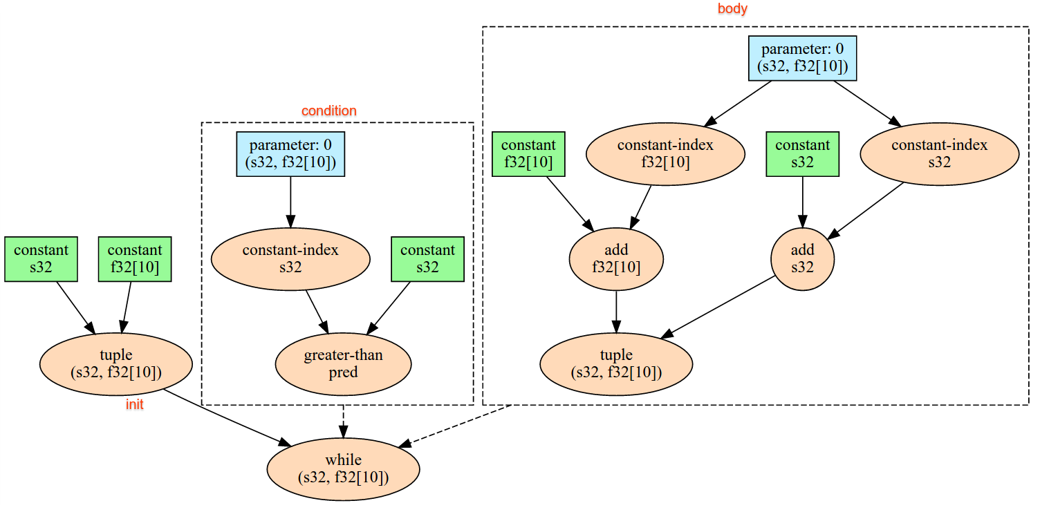
XlaOp מהנתונים. בחישוב של מספר פעולות אפשר לבצע פעולות מרובות בגוף הפיד, אבל חייבת להיות סדר כולל בין הפעולות. לדוגמה, לשתי מודעות בגוף הפיד בקוד שבהמשך יש סדר כולל, כי יש תלות בין לולאות ה-\n.
result1 = while (condition, init = init_value) {
  Infeed(shape)
}

result2 = while (condition, init = result1) {
  Infeed(shape)
}
אין תמיכה בצורות זוגיות מקוננות. במקרה של צורה כפולה ריקה, הפעולה בתוך הפיד לא מאפשרת לבצע פעולות וממשיכה בלי לקרוא נתונים מהפיד של המכשיר.
Iota
למידע נוסף: XlaBuilder::Iota.
Iota(shape, iota_dimension)
יוצרת ליטרל קבוע במכשיר במקום העברה פוטנציאלית של מארח
גדול. יוצרת מערך עם צורה מוגדרת ומאחסן ערכים המתחילים באפס ומצטברים באחד במאפיין שצוין. לסוגים של נקודה צפה (floating-point), המערך שנוצר שווה ערך ל-ConvertElementType(Iota(...)), שבו Iota הוא מסוג אינטגרלי וההמרה היא מסוג נקודה צפה (floating-point).
| ארגומנטים | סוג | סמנטיקה |
|---|---|---|
shape |
Shape |
צורת המערך שנוצר על ידי Iota() |
iota_dimension |
int64 |
המאפיין שיש להוסיף. |
לדוגמה, הפונקציה Iota(s32[4, 8], 0) מחזירה
  [[0, 0, 0, 0, 0, 0, 0, 0 ],
   [1, 1, 1, 1, 1, 1, 1, 1 ],
   [2, 2, 2, 2, 2, 2, 2, 2 ],
   [3, 3, 3, 3, 3, 3, 3, 3 ]]
אפשרות החזרה במחיר Iota(s32[4, 8], 1)
  [[0, 1, 2, 3, 4, 5, 6, 7 ],
   [0, 1, 2, 3, 4, 5, 6, 7 ],
   [0, 1, 2, 3, 4, 5, 6, 7 ],
   [0, 1, 2, 3, 4, 5, 6, 7 ]]
מפה
למידע נוסף: XlaBuilder::Map.
Map(operands..., computation)
| ארגומנטים | סוג | סמנטיקה |
|---|---|---|
operands |
רצף של N XlaOp שנ' |
N מערכים של סוגים T0..T{N-1} |
computation |
XlaComputation |
חישוב מסוג T_0, T_1, .., T_{N + M -1} -> S עם N פרמטרים מסוג T ו-M מסוג שרירותי |
dimensions |
מערך int64 |
מערך ממדי מפה |
מחילה פונקציה סקלרית על מערכי operands הנתונים, ויוצרת מערך של אותם מאפיינים כאשר כל רכיב הוא תוצאה של הפונקציה הממופה שהוחלה על הרכיבים התואמים במערכי הקלט.
הפונקציה הממופה היא חישוב שרירותי עם ההגבלה שיש לה N קלטים מסוג סקלרי T ופלט יחיד מסוג S. לפלט יש אותם מימדים כמו האופרנדים, אלא שסוג הרכיב T מוחלף ב-S.
לדוגמה: Map(op1, op2, op3, computation, par1) ממפה את elem_out <-
computation(elem1, elem2, elem3, par1) בכל אינדקס (רב-ממדי) במערכי הקלט כדי להפיק את מערך הפלט.
OptimizationBarrier
חסימת כל מעבר אופטימיזציה להעברת חישובים דרך המחסום.
הפונקציה מבטיחה שכל ערכי הקלט ייבדקו לפני אופרטורים שתלויים בפלט של המחסום.
רפידה
למידע נוסף: XlaBuilder::Pad.
Pad(operand, padding_value, padding_config)
| ארגומנטים | סוג | סמנטיקה |
|---|---|---|
operand |
XlaOp |
מערך מסוג T |
padding_value |
XlaOp |
סקלרי מסוג T למילוי המרווח הנוסף |
padding_config |
PaddingConfig |
מידת המרווח הפנימי בשני הקצוות (נמוך, גבוה) ובין הרכיבים של כל מימד |
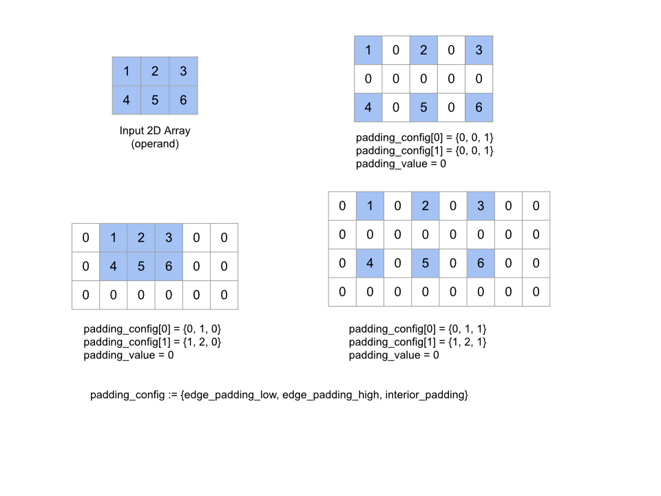
מרחיבה את המערך operand הנתון באמצעות מרווח פנימי סביב המערך וכן בין הרכיבים של המערך עם ה-padding_value הנתון. padding_config
מציין את המרווח הפנימי בקצוות ואת המרווח הפנימי של כל מימד.
PaddingConfig הוא שדה חוזר של PaddingConfigDimension, שמכיל שלושה שדות לכל מאפיין: edge_padding_low, edge_padding_high ו-interior_padding.
edge_padding_low ו-edge_padding_high מציינים את כמות המרווח הפנימי שנוספה ברמה הנמוכה (לצד אינדקס 0) ובחלק העליון (לצד האינדקס הגבוה ביותר) של כל מאפיין, בהתאמה. מידת המרווח פנימי בקצוות יכולה להיות שלילית. הערך המוחלט של מרווח פנימי שלילי מציין את מספר הרכיבים שיש להסיר מהמאפיין שצוין.
interior_padding מציין את כמות המרווח הפנימי שנוסף בין שני רכיבים בכל מאפיין. הוא לא יכול להיות שלילי. המרווח הפנימי מופיע באופן הגיוני לפני המרווח הפנימי בקצוות, כך שבמקרה של מרווח שלילי בקצוות, האלמנטים יוסרו מהאופרנד עם הריפוד הפנימי.
הפעולה הזו היא "no-op" אם כל זוגות המרווח הפנימי של הקצוות הם (0, 0) וערכים של מרווח פנימי פנימיים הם כולם 0. באיור הבא מוצגות דוגמאות לערכים שונים של edge_padding ו-interior_padding למערך דו ממדי.
הקלטה
למידע נוסף: XlaBuilder::Recv.
Recv(shape, channel_handle)
| ארגומנטים | סוג | סמנטיקה |
|---|---|---|
shape |
Shape |
הצורה של הנתונים לקבל |
channel_handle |
ChannelHandle |
מזהה ייחודי לכל צמד שליחה/הקלטה |
הפונקציה מקבלת נתונים של צורה מסוימת מהוראה של Send בחישוב אחר שיש לו אותו מזהה ערוץ. הפונקציה מחזירה
XlaOp את הנתונים שהתקבלו.
הפעולה Recv של ממשק ה-API של הלקוח מייצגת תקשורת סנכרונית.
עם זאת, ההוראה מחולקת באופן פנימי לשתי הוראות HLO (Recv ו-RecvDone) כדי לאפשר העברות אסינכרוניות של נתונים. למידע נוסף: HloInstruction::CreateRecv ו-HloInstruction::CreateRecvDone.
Recv(const Shape& shape, int64 channel_id)
הפונקציה משייכת את המשאבים שדרושים כדי לקבל נתונים מהוראה ל-Send עם אותו channel_id. מחזירה הקשר למשאבים שהוקצו. הוראה זו משתמשת בהוראה הבאה של RecvDone להמתנה להשלמת העברת הנתונים. ההקשר הוא שילוב של {receive buffer (shape), request request (U32)} (מזהה בקשה למאגר נתונים) (U32)} ואפשר להשתמש בו רק באמצעות הוראה RecvDone.
RecvDone(HloInstruction context)
בהתאם להקשר שנוצר על ידי הוראה Recv, צריך להמתין להשלמת העברת הנתונים ולהחזיר את הנתונים שהתקבלו.
הקטנה
למידע נוסף: XlaBuilder::Reduce.
מחילה פונקציית הפחתה על מערך אחד או יותר במקביל.
Reduce(operands..., init_values..., computation, dimensions)
| ארגומנטים | סוג | סמנטיקה |
|---|---|---|
operands |
רצף של N XlaOp |
N מערכים מסוג T_0, ..., T_{N-1}. |
init_values |
רצף של N XlaOp |
N סקלר מסוגי T_0, ..., T_{N-1}. |
computation |
XlaComputation |
חישוב מסוג T_0, ..., T_{N-1}, T_0, ..., T_{N-1} -> Collate(T_0, ..., T_{N-1}). |
dimensions |
מערך int64 |
מערך לא מסודר של מימדים שיש לצמצם. |
כאשר:
- N חייב להיות גדול מ-1 או שווה לו.
- החישוב צריך להיות אסוציאטיבי "בערך" (ראו בהמשך).
- כל מערכי הקלט חייבים להיות בעלי מימדים זהים.
- כל הערכים הראשוניים צריכים ליצור זהות במסגרת
computation. - אם
N = 1, הערך שלCollate(T)הואT. - אם
N > 1, הערךCollate(T_0, ..., T_{N-1})הוא צירוף שלNרכיבים מסוגT.
פעולה זו מצמצמת מאפיין אחד או יותר של כל מערך קלט לסקלרים.
הדירוג של כל מערך שמוחזר הוא rank(operand) - len(dimensions). הפלט של הפעולה הוא Collate(Q_0, ..., Q_N) כאשר Q_i הוא מערך מסוג T_i, שהמאפיינים שלהם מתוארים בהמשך.
מותר לשייך מחדש את חישוב ההפחתה בקצוות עורפיים שונים. זה יכול להוביל להבדלים מספריים, כי חלק מפונקציות ההפחתה, כמו חיבור, לא אסוציאטיביות של ערכים צפים. עם זאת, אם טווח הנתונים מוגבל, הוספה של נקודה צפה (floating-point) קרובה למדי כדי שתהיה אסוציאטיבית לרוב השימושים המעשיים.
דוגמאות
כשמצמצמים מאפיין אחד במערך חד-ממדי אחד עם הערכים [10, 11,
12, 13], עם פונקציית ההפחתה f (כלומר computation), אפשר לחשב אותו כך:
f(10, f(11, f(12, f(init_value, 13)))
אבל יש גם אפשרויות רבות אחרות,
f(init_value, f(f(10, f(init_value, 11)), f(f(init_value, 12), f(init_value, 13))))
לפניכם דוגמה לפסאודו-קוד כללי של האופן שבו ניתן ליישם את ההפחתה, תוך שימוש בסכימה בתור חישוב ההפחתה עם ערך ראשוני של 0.
result_shape <- remove all dims in dimensions from operand_shape

# Iterate over all elements in result_shape. The number of r's here is equal
# to the rank of the result
for r0 in range(result_shape[0]), r1 in range(result_shape[1]), ...:
  # Initialize this result element
  result[r0, r1...] <- 0

  # Iterate over all the reduction dimensions
  for d0 in range(dimensions[0]), d1 in range(dimensions[1]), ...:
    # Increment the result element with the value of the operand's element.
    # The index of the operand's element is constructed from all ri's and di's
    # in the right order (by construction ri's and di's together index over the
    # whole operand shape).
    result[r0, r1...] += operand[ri... di]
כאן מוצגת דוגמה להפחתת מערך דו-ממדי (מטריצה). לצורה יש דירוג 2, מאפיין 0 בגודל 2 ומאפיין 1 בגודל 3:
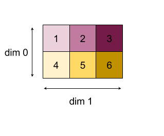
תוצאות של הפחתת מאפיינים 0 או 1 באמצעות פונקציית "add":
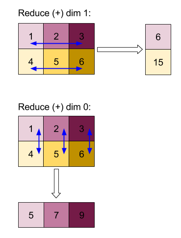
שימו לב ששתי תוצאות ההפחתה הן מערכים חד-ממדיים. בתרשים מוצגות עמודה אחת כעמודה ואחרת כשורה מטעמי נוחות.
הנה דוגמה מורכבת יותר. הדירוג שלה הוא 3, מאפיין 0 גודל 4, מאפיין 1 בגודל 2 ומאפיין 2 בגודל 3. כדי לפשט את הדברים, הערכים 1 עד 6 משוכפלים במאפיין 0.
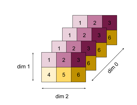
בדומה לדוגמה הדו-ממדית, אנחנו יכולים להפחית מימד אחד בלבד. אם מפחיתים את מאפיין 0, לדוגמה, מקבלים מערך דירוג 2 שבו כל הערכים של מאפיין 0 מקופלים לסקלרי:
|  4   8  12 |
| 16  20  24 |
אם מפחיתים את מאפיין 2, מקבלים גם מערך דירוג 2 שבו כל הערכים של מאפיין 2 מקופלים לסקלרי:
| 6  15 |
| 6  15 |
| 6  15 |
| 6  15 |
שימו לב שהסדר היחסי בין שאר המאפיינים בקלט נשמר בפלט, אבל ייתכן שלמאפיינים מסוימים יוקצו מספרים חדשים (כי הדירוג משתנה).
כמו כן, אנחנו יכולים לצמצם מספר מאפיינים. כשמחברים את מידות 0 ו-1 נוצר המערך החד-ממדי [20, 28, 36].
הקטנת המערך התלת-ממדי בכל המידות שלו יוצרת את 84 הסקלרי.
צמצום וראיאדית
ב-N > 1, הפחתת השימוש של הפונקציה היא קצת יותר מורכבת, כי מחילים אותה בו-זמנית על כל ערכי הקלט. האופרנדים מסופקים לחישוב לפי הסדר הבא:
- הרצת ערך מופחת של האופרנד הראשון
- ...
- הרצת ערך מופחת של אופרנד N
- ערך קלט לאופרנד הראשון
- ...
- ערך קלט לאופרנד N
לדוגמה, נשתמש בפונקציית ההפחתה הבאה, שבה ניתן להשתמש כדי לחשב במקביל את ערכי המקסימום ואת ה-argmax של מערך 1-D:
f: (Float, Int, Float, Int) -> Float, Int
f(max, argmax, value, index):
  if value >= max:
    return (value, index)
  else:
    return (max, argmax)
במקרה של מערכי קלט חד-ממדיים V = Float[N], K = Int[N], וערכי התחילית I_V = Float, I_K = Int, התוצאה f_(N-1) של צמצום במאפיין הקלט היחיד מקבילה ליישום הרקורסיבי הבא:
f_0 = f(I_V, I_K, V_0, K_0)
f_1 = f(f_0.first, f_0.second, V_1, K_1)
...
f_(N-1) = f(f_(N-2).first, f_(N-2).second, V_(N-1), K_(N-1))
החלת ההפחתה הזו על מערך של ערכים ומערך של אינדקסים רציפים (כלומר iota), תעבור חזרה על המערכים ותחזיר טופס כפול שמכיל את הערך המקסימלי ואת האינדקס התואם.
ReducePrecision
למידע נוסף: XlaBuilder::ReducePrecision.
הדגמה של ההשפעה של המרת ערכים של נקודה צפה (floating-point) לפורמט ברמת דיוק נמוכה יותר (כמו IEEE-FP16) וחזרה לפורמט המקורי. אפשר לציין באופן שרירותי את מספר הביטים המעריך והמנטיסה בפורמט ברמת דיוק נמוכה יותר, למרות שיכול להיות שלא כל גודלי הביטים נתמכים בכל הטמעות החומרה.
ReducePrecision(operand, mantissa_bits, exponent_bits)
| ארגומנטים | סוג | סמנטיקה |
|---|---|---|
operand |
XlaOp |
מערך של נקודה צפה מסוג T. |
exponent_bits |
int32 |
מספר הביטים בהערכה בפורמט דיוק נמוך יותר |
mantissa_bits |
int32 |
מספר ביטים מנטיסה בפורמט ברמת דיוק נמוכה יותר |
התוצאה היא מערך מסוג T. ערכי הקלט מעוגלים לערך הקרוב ביותר שניתן לייצוג עם מספר הביטים של מנטיסה (באמצעות "מקשרים לסמנטיקה"), וכל הערכים שחורגים מהטווח שצוין במספר הביטים המעריכים מוצמדים לאינסוף חיובי או שלילי. ערכי NaN
נשמרים, אבל יכול להיות שהם יומרו לערכים קנוניים של NaN.
הפורמט ברמת דיוק נמוכה יותר צריך לכלול לפחות ביט אחד של מעריך (כדי להבחין בין ערך אפס לאינסוף, מכיוון ששניהם בעלי אפס מנטיסה), וחייב להיות לו מספר לא שלילי של ביטים. מספר הביטים מסוג 'מעריך' או 'המנטיסה' עשוי להיות גבוה מהערך המתאים לסוג T. החלק המתאים של ההמרה הוא פשוט אי-פעולה.
ReduceScatter
למידע נוסף: XlaBuilder::ReduceScatter.
פונקציית DecreaseScatter היא פעולה קולקטיבית שמבצעת ביעילות פעולה של AllDecrease, ואז מפצלת את התוצאה לבלוקים של shard_count לאורך ה-scatter_dimension, והעותק i בקבוצת העותקים מקבלת את הפיצול ith.
ReduceScatter(operand, computation, scatter_dim, shard_count,
replica_group_ids, channel_id)
| ארגומנטים | סוג | סמנטיקה |
|---|---|---|
operand |
XlaOp |
מערך או צמד לא ריק של מערכים לצמצום בין רפליקות. |
computation |
XlaComputation |
חישוב הפחתה |
scatter_dimension |
int64 |
גודל לפיזור. |
shard_count |
int64 |
מספר הבלוקים לפיצול scatter_dimension |
replica_groups |
את הווקטורים של int64 |
קבוצות שביניהן מתבצע ההפחתה |
channel_id |
ערך אופציונלי של int64 |
מזהה ערוץ אופציונלי לתקשורת בין מודולים |
- כשהערך הוא
operandב-tuple של מערכים, מתבצע פונקציית הפיזור על כל רכיב ב-tuple. replica_groupsהיא רשימה של קבוצות של עותקים שביניהן מתבצעת ההפחתה (אפשר לאחזר מזהה עותק של הרפליקה הנוכחית באמצעותReplicaId). סדר הרפליקות בכל קבוצה קובע את הסדר שבו תתפזר התוצאה הכוללת של כל הפחתה. השדהreplica_groupsחייב להיות ריק (במקרה כזה, כל הרפליקות שייכות לקבוצה אחת) או להכיל את אותו מספר רכיבים כמו מספר הרפליקות. כשיש יותר מקבוצה אחת של רפליקות, כולן חייבות להיות באותו גודל. לדוגמה, הפונקציהreplica_groups = {0, 2}, {1, 3}מבצעת הפחתה בין העותקים0ו-2, ו-1ו-3ואז מפזרת את התוצאה.shard_countהוא הגודל של כל קבוצת עותקים. צריך להשתמש בה במקרים שבהם השדהreplica_groupsריק. אם השדהreplica_groupsלא ריק, הערך שלshard_countחייב להיות שווה לגודל של כל קבוצת עותקים.channel_idמשמש לתקשורת בין מודולים: רק פעולותreduce-scatterעם אותוchannel_idיכולות לתקשר זו עם זו.
צורת הפלט היא צורת הקלט כאשר scatter_dimension קטן פי shard_count. לדוגמה, אם יש שני רפליקות והאופרנד מכיל את הערך [1.0, 2.25] ו-[3.0, 5.25] בהתאמה בשני העתקים, ערך הפלט מהפעולה הזו שבו scatter_dim הוא 0 יהיה [4.0] לעותק הראשון ו-[7.5] לעותק השני.
ReduceWindow
למידע נוסף: XlaBuilder::ReduceWindow.
מחילה פונקציית הפחתה על כל הרכיבים בכל חלון של רצף N מערכים רב-ממדיים, וכך יוצרת פלט של N מערכים רב-ממדיים באופן יחיד או כפול. לכל מערך פלט יש מספר הרכיבים זהה למספר המיקומים החוקיים של החלון. ניתן לבטא שכבת מאגר כ-ReduceWindow. בדומה ל-Reduce, computation שהוחל תמיד עובר את ה-init_values בצד שמאל.
ReduceWindow(operands..., init_values..., computation, window_dimensions,
window_strides, padding)
| ארגומנטים | סוג | סמנטיקה |
|---|---|---|
operands |
N XlaOps |
רצף של N מערכים רב-ממדיים מסוג T_0,..., T_{N-1}, שכל אחד מהם מייצג את אזור הבסיס שעליו ממוקם החלון. |
init_values |
N XlaOps |
ערכי ההתחלה של N עבור ההפחתה, אחד לכל אופרנד N. פרטים נוספים זמינים במאמר הפחתה. |
computation |
XlaComputation |
פונקציית הפחתה מסוג T_0, ..., T_{N-1}, T_0, ..., T_{N-1} -> Collate(T_0, ..., T_{N-1}), להחלה על רכיבים בכל חלון של כל אופרנד הקלט. |
window_dimensions |
ArraySlice<int64> |
מערך של מספרים שלמים לערכי המימדים של החלון |
window_strides |
ArraySlice<int64> |
מערך של מספרים שלמים לערכי רוחב החלון |
base_dilations |
ArraySlice<int64> |
מערך של מספרים שלמים לערכי הרחבת בסיס |
window_dilations |
ArraySlice<int64> |
מערך של מספרים שלמים לערכים של הרחבת חלון |
padding |
Padding |
סוג המרווח הפנימי של חלון (ריפוד::kSame, המשטח את הפלט כדי שיהיה זהה לצורת הפלט כמו הקלט אם הצלע היא 1, או Padding::kValid, שלא משתמש במרווח פנימי ו "מעצור" את החלון כשהוא לא מתאים יותר) |
כאשר:
- N חייב להיות גדול מ-1 או שווה לו.
- כל מערכי הקלט חייבים להיות בעלי מימדים זהים.
- אם
N = 1, הערך שלCollate(T)הואT. - אם
N > 1, הערךCollate(T_0, ..., T_{N-1})הוא צירוף שלNרכיבים מסוג(T0,...T{N-1}).
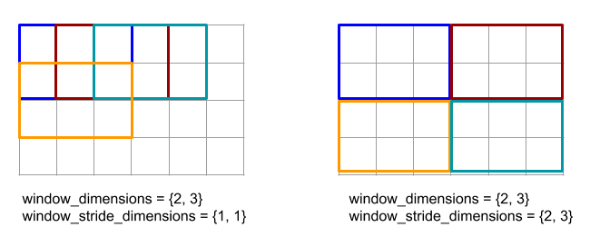
הקוד והאיור שלמטה מראים דוגמה לשימוש ב-ReduceWindow. הקלט הוא מטריצה בגודל [4x6], וגם window_dimensions ו-window_stride_dimensions הם [2x3].
// Create a computation for the reduction (maximum).
XlaComputation max;
{
  XlaBuilder builder(client_, "max");
  auto y = builder.Parameter(0, ShapeUtil::MakeShape(F32, {}), "y");
  auto x = builder.Parameter(1, ShapeUtil::MakeShape(F32, {}), "x");
  builder.Max(y, x);
  max = builder.Build().value();
}

// Create a ReduceWindow computation with the max reduction computation.
XlaBuilder builder(client_, "reduce_window_2x3");
auto shape = ShapeUtil::MakeShape(F32, {4, 6});
auto input = builder.Parameter(0, shape, "input");
builder.ReduceWindow(
    input,
    /*init_val=*/builder.ConstantLiteral(LiteralUtil::MinValue(F32)),
    *max,
    /*window_dimensions=*/{2, 3},
    /*window_stride_dimensions=*/{2, 3},
    Padding::kValid);
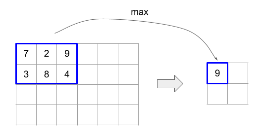
שלב 1 במאפיין מציין שהמיקום של חלון במאפיין נמצא במרחק של רכיב אחד מהחלון הצמוד שלו. כדי לציין שאין חלונות שחופפים זה לזה, המאפיין window_stride_dimensions צריך להיות שווה ל-window_dimensions. האיור שלמטה ממחיש את השימוש בשני ערכי צעדים שונים. המרווח מוחל על כל מאפיין של הקלט, והחישובים זהים לאופן שבו הקלט נכנס עם המימדים שיש לו אחרי המרווח.
בדוגמה של מרווח פנימי לא טריוויאלי, כדאי לחשב את הערך המינימלי של חלונות מצמצמים (הערך הראשוני הוא MAX_FLOAT) עם המאפיין 3 ולעבור 2 למערך הקלט [10000, 1000, 100, 10, 1]. באמצעות המרווח של kValid, המערכת מחשבת מינימום לשני חלונות חוקיים: [10000, 1000, 100] ו-[100, 10, 1], וכך מתקבל הערך [100, 1] בפלט. לאחר המרווח של kSame, המערך נוצר כך שהצורה שאחרי החלון הקטן תהיה זהה לקלט בשלב הראשון, על ידי הוספת רכיבים ראשוניים בשני הצדדים, כדי לקבל [MAX_VALUE, 10000, 1000, 100, 10, 1,
MAX_VALUE]. הרצה של חלונות עם חלונות קטנים על המערך המרופד פועלת בשלושה חלונות [MAX_VALUE, 10000, 1000], [1000, 100, 10], [10, 1, MAX_VALUE] ו-[1000, 10, 1].
סדר ההערכה של פונקציית ההפחתה הוא שרירותי, ועשוי להיות לא דטרמיני. לכן, פונקציית ההפחתה לא צריכה להיות רגישה מדי לשיוך מחדש. לפרטים נוספים, כדאי לקרוא את הדיון על אסוציאטיביות בהקשר של Reduce.
ReplicaId
למידע נוסף: XlaBuilder::ReplicaId.
מחזירה את המזהה הייחודי (U32 סקלרי) של העותק.
ReplicaId()
המזהה הייחודי של כל עותק הוא מספר שלם לא חתום במרווח הזמן [0, N), כאשר N הוא מספר הרפליקות. מכיוון שכל הרפליקות פועלות באותה תוכנית, קריאה ל-ReplicaId() בתוכנית תחזיר ערך שונה בכל עותק.
שינוי הצורה
למידע נוסף, ראו XlaBuilder::Reshape והפעולה Collapse.
הפונקציה הופכת את המידות של מערך למערך חדש.
Reshape(operand, new_sizes)
Reshape(operand, dimensions, new_sizes)
| ארגומנטים | סוג | סמנטיקה |
|---|---|---|
operand |
XlaOp |
מערך מסוג T |
dimensions |
וקטור int64 |
הסדר שבו המאפיינים מכווצים |
new_sizes |
וקטור int64 |
וקטור גדלים של מאפיינים חדשים |
באופן עקרוני, תחילה צריך לעצב מחדש מערך כדי ליצור לו וקטור חד-ממדי של ערכי נתונים, ולאחר מכן לצמצם אותו לצורה חדשה. הארגומנטים של הקלט הם מערך שרירותי מסוג T, וקטור קבוע של מאפיינים עם זמן הידור ווקטורים של גודלי מאפיינים עבור התוצאה.
הערכים בווקטור dimension, אם הם מוגדרים, צריכים להיות פרמוטציה של כל מאפייני ה-T. ברירת המחדל אם היא לא נתונה היא {0, ..., rank - 1}. הסדר של המאפיינים ב-dimensions הוא ממאפיין עם המשתנה האיטי ביותר (העיקרי) למימד המשתנות במהירות ביותר (הכי משני) ב-Nest Nest, כדי לכווץ את מערך הקלט למאפיין יחיד. הווקטור new_sizes קובע את הגודל של מערך הפלט. הערך באינדקס 0 ב-new_sizes הוא הגודל של מאפיין 0, הערך באינדקס 1 הוא גודל מאפיין 1 וכן הלאה. המכפלה של מידות new_size חייבת להיות שווה למכפלה של גודלי המאפיינים של האופרנד. כשמשפרים את המערך המכווץ למערך רב-ממדי שהוגדר על ידי new_sizes, המאפיינים ב-new_sizes מסודרים מהמשתנה האיטי ביותר (העיקרי) ומהמשתנה המהיר ביותר (המשני ביותר).
לדוגמה, מגדירים את v כמערך של 24 רכיבים:
let v = f32[4x2x3] { { {10, 11, 12}, {15, 16, 17} },
                    { {20, 21, 22}, {25, 26, 27} },
                    { {30, 31, 32}, {35, 36, 37} },
                    { {40, 41, 42}, {45, 46, 47} } };

In-order collapse:
let v012_24 = Reshape(v, {0,1,2}, {24});
then v012_24 == f32[24] {10, 11, 12, 15, 16, 17, 20, 21, 22, 25, 26, 27,
                         30, 31, 32, 35, 36, 37, 40, 41, 42, 45, 46, 47};

let v012_83 = Reshape(v, {0,1,2}, {8,3});
then v012_83 == f32[8x3] { {10, 11, 12}, {15, 16, 17},
                          {20, 21, 22}, {25, 26, 27},
                          {30, 31, 32}, {35, 36, 37},
                          {40, 41, 42}, {45, 46, 47} };

Out-of-order collapse:
let v021_24 = Reshape(v, {1,2,0}, {24});
then v012_24 == f32[24]  {10, 20, 30, 40, 11, 21, 31, 41, 12, 22, 32, 42,
                          15, 25, 35, 45, 16, 26, 36, 46, 17, 27, 37, 47};

let v021_83 = Reshape(v, {1,2,0}, {8,3});
then v021_83 == f32[8x3] { {10, 20, 30}, {40, 11, 21},
                          {31, 41, 12}, {22, 32, 42},
                          {15, 25, 35}, {45, 16, 26},
                          {36, 46, 17}, {27, 37, 47} };


let v021_262 = Reshape(v, {1,2,0}, {2,6,2});
then v021_262 == f32[2x6x2] { { {10, 20}, {30, 40},
                              {11, 21}, {31, 41},
                              {12, 22}, {32, 42} },
                             { {15, 25}, {35, 45},
                              {16, 26}, {36, 46},
                              {17, 27}, {37, 47} } };
במקרה מיוחד, reshape יכול להפוך מערך עם רכיב יחיד לסקלרי ולהפך. לדוגמה,
Reshape(f32[1x1] { {5} }, {0,1}, {}) == 5;
Reshape(5, {}, {1,1}) == f32[1x1] { {5} };
Rev (היפוך)
למידע נוסף: XlaBuilder::Rev.
Rev(operand, dimensions)
| ארגומנטים | סוג | סמנטיקה |
|---|---|---|
operand |
XlaOp |
מערך מסוג T |
dimensions |
ArraySlice<int64> |
מימדים להיפוך |
הפונקציה הופכת את סדר הרכיבים במערך operand לאורך
dimensions שצוין, ויוצרת מערך פלט של אותה צורה. כל רכיב במערך האופרנד באינדקס רב-ממדי מאוחסן במערך הפלט באינדקס שעבר שינוי. האינדקס הרב-ממדי משתנה על ידי היפוך האינדקס בכל אחד מהמאפיינים להיפוך (כלומר, אם מימד בגודל N הוא אחד
ממאפייני ההיפוך, האינדקס i שלו משתנה ל-N - 1 - i).
אחד השימושים בפעולה Rev הוא להפוך את מערך משקל הקונבולוציה לאורך שני ממדי החלון במהלך חישוב ההדרגתיות ברשתות נוירונים.
RngNormal
למידע נוסף: XlaBuilder::RngNormal.
בונה פלט של צורה נתונה עם מספרים אקראיים שנוצרים אחרי ההתפלגות הנורמלית \(N(\mu, \sigma)\) . הפרמטרים \(\mu\) ו- \(\sigma\)וצורת הפלט צריכים להיות מסוג אלמנטים של נקודה צפה (floating-point). לפרמטרים נוספים יש ערך סקלרי.
RngNormal(mu, sigma, shape)
| ארגומנטים | סוג | סמנטיקה |
|---|---|---|
mu |
XlaOp |
סולם מסוג T שמציין את הממוצע של המספרים שנוצרו |
sigma |
XlaOp |
סולם מסוג T שמציין סטיית תקן של |
shape |
Shape |
צורת פלט מסוג T |
RngUniform
למידע נוסף: XlaBuilder::RngUniform.
הפונקציה בונה פלט של צורה נתונה עם מספרים אקראיים שנוצרים בעקבות ההתפלגות האחידה על פני המרווח \([a,b)\). הפרמטרים וסוג הרכיב הפלט צריכים להיות מסוג בוליאני, סוג אינטגרל או סוגי נקודות צפות, והסוגים חייבים להיות עקביים. הקצוות העורפיים של המעבד (CPU) וה-GPU תומכים כרגע רק בדגמים F64, F32, F16, BF16, S64, U64, S32 ו-U32. בנוסף, צריך להקצות ערך סקלרי לפרמטרים. אם \(b <= a\) התוצאה מוגדרת כהטמעה.
RngUniform(a, b, shape)
| ארגומנטים | סוג | סמנטיקה |
|---|---|---|
a |
XlaOp |
סולם מסוג T שמציין גבול תחתון של מרווח |
b |
XlaOp |
סולם מסוג T שמציין גבול עליון של מרווח |
shape |
Shape |
צורת פלט מסוג T |
RngBitGenerator
יוצרת פלט עם צורה נתונה שמתמלאת בביטים אקראיים אחידים באמצעות האלגוריתם שצוין (או בברירת המחדל של הקצה העורפי), ומחזירה מצב מעודכן (עם אותה צורה כמו המצב הראשוני) ואת הנתונים האקראיים שנוצרו.
המצב ההתחלתי הוא המצב הראשוני של יצירת המספרים האקראיים הנוכחיים. המאפיין הזה, הצורה והערכים החוקיים הנדרשים תלויים באלגוריתם שבו נעשה שימוש.
מובטח שהפלט יהיה פונקציה דטרמיניסטית של המצב הראשוני, אבל לא בטוח שהוא יהיה דטרמיניסטי בין קצוות עורפיים וגרסאות מהדר שונות.
RngBitGenerator(algorithm, key, shape)
| ארגומנטים | סוג | סמנטיקה |
|---|---|---|
algorithm |
RandomAlgorithm |
יש להשתמש באלגוריתם PRNG. |
initial_state |
XlaOp |
מצב ראשוני של אלגוריתם PRNG. |
shape |
Shape |
צורת הפלט של הנתונים שנוצרים. |
הערכים הזמינים עבור algorithm:
rng_default: אלגוריתם ספציפי לקצה העורפי ודרישות צורה ספציפיות לקצה העורפי.rng_three_fry: אלגוריתם PRNG של ThreeFry המבוסס על מונה. הצורהinitial_stateהיאu64[2]עם ערכים שרירותיים. Salmon et al. SC 2011. מספרים אקראיים מקבילים: קלים כמו 1, 2 ו-3.rng_philox: אלגוריתם Philox ליצירת מספרים אקראיים במקביל. הצורהinitial_stateהיאu64[3]עם ערכים שרירותיים. Salmon et al. SC 2011. מספרים אקראיים מקבילים: קלים כמו 1, 2 ו-3.
פיזור
פעולת הפיזור XLA יוצרת רצף של תוצאות שהן הערכים
של מערך הקלט operands, עם מספר פלחים (באינדקסים שצוינו על ידי scatter_indices) שעודכנו לפי רצף הערכים ב-updates באמצעות update_computation.
למידע נוסף: XlaBuilder::Scatter.
scatter(operands..., scatter_indices, updates..., update_computation,
index_vector_dim, update_window_dims, inserted_window_dims,
scatter_dims_to_operand_dims)
| ארגומנטים | סוג | סמנטיקה |
|---|---|---|
operands |
רצף של N XlaOp |
N מערכים מסוג T_0, ..., T_N לפיזור בהם. |
scatter_indices |
XlaOp |
מערך שמכיל את האינדקסים הראשונים של הפרוסות שצריך לפזר אליהן. |
updates |
רצף של N XlaOp |
N מערכים מסוג T_0, ..., T_N. updates[i] מכיל את הערכים שצריך להשתמש בהם לפיזור operands[i]. |
update_computation |
XlaComputation |
חישוב לשלב בין הערכים הקיימים במערך הקלט לבין העדכונים במהלך הפיזור. החישוב הזה צריך להיות מסוג T_0, ..., T_N, T_0, ..., T_N -> Collate(T_0, ..., T_N). |
index_vector_dim |
int64 |
המאפיין ב-scatter_indices שמכיל את האינדקסים המתחילים. |
update_window_dims |
ArraySlice<int64> |
קבוצת המאפיינים בצורה updates שהם מידות של חלונות. |
inserted_window_dims |
ArraySlice<int64> |
קבוצת מידות החלונות שיש להכניס לצורת updates. |
scatter_dims_to_operand_dims |
ArraySlice<int64> |
מפת מימדים מאינדקס הפיזור אל מרחב אינדקס האופרנד. המערך הזה מפוענח כמיפוי i ל-scatter_dims_to_operand_dims[i] . העדכון חייב להיות אחד לאחד ובסך הכול. |
indices_are_sorted |
bool |
האם מובטחת שהאינדקסים ימוינו על ידי מבצע הקריאה. |
כאשר:
- N חייב להיות גדול מ-1 או שווה לו.
operands[0], ...,operands[N-1] צריכים להיות בעלי אותם מאפיינים.updates[0], ...,updates[N-1] צריכים להיות בעלי אותם מאפיינים.- אם
N = 1, הערך שלCollate(T)הואT. - אם
N > 1, הערךCollate(T_0, ..., T_N)הוא צמד שלNרכיבים מסוגT.
אם index_vector_dim שווה ל-scatter_indices.rank, אנחנו גם מחשיבים באופן לא מפורש
ל-scatter_indices את המאפיין 1 בסוף.
אנחנו מגדירים update_scatter_dims מסוג ArraySlice<int64> כקבוצת המאפיינים בצורה updates שאינם ב-update_window_dims, בסדר עולה.
הארגומנטים של פיזור צריכים להתאים למגבלות הבאות:
כל מערך
updatesחייב להיות מהדירוגupdate_window_dims.size + scatter_indices.rank - 1.גבולות המאפיין
iבכל מערךupdatesצריכים להיות תואמים לתנאים הבאים:- אם
iקיים ב-update_window_dims(כלומר שווה ל-update_window_dims[k] עבור חלק מ-k), אז הגבול של המאפייןiב-updatesלא יכול להיות גדול מהגבול התואם שלoperandאחרי חשבוןinserted_window_dims(כלומרadjusted_window_bounds[k], שבוadjusted_window_boundsמכיל את הגבולות שלoperandעם הסרת הגבולות באינדקסיםinserted_window_dims). - אם
iקיים ב-update_scatter_dims(כלומר שווה ל-update_scatter_dims[k] עבור חלק מ-k), אז הגבול של המאפייןiב-updatesחייב להיות שווה לגבול התואם שלscatter_indices, והוא מדלג עלindex_vector_dim(כלומרscatter_indices.shape.dims[k], אםk<index_vector_dimו-scatter_indices.shape.dims[k+1] אחרת).
- אם
הערך
update_window_dimsחייב להופיע בסדר עולה, ללא מספרי מאפיינים חוזרים והוא צריך להיות בטווח[0, updates.rank).הערך
inserted_window_dimsחייב להופיע בסדר עולה, ללא מספרי מאפיינים חוזרים והוא צריך להיות בטווח[0, operand.rank).operand.rankחייב להיות שווה לסכום שלupdate_window_dims.sizeו-inserted_window_dims.size.scatter_dims_to_operand_dims.sizeחייב להיות שווה ל-scatter_indices.shape.dims[index_vector_dim] והערכים שלו צריכים להיות בטווח[0, operand.rank).
לאינדקס נתון U בכל מערך updates, מחושב האינדקס התואם I במערך operands המתאים שאליו יש להחיל את העדכון באופן הבא:
- הפונקציה
G= {U[k] עבורkב-update_scatter_dims}. אפשר להשתמש ב-Gכדי לחפש וקטור אינדקסSבמערךscatter_indices, כך ש-S[i] =scatter_indices[שילוב(G,i)] שבו שילוב(A, b) יוסיף את b במיקומיםindex_vector_dimל-A. - אפשר ליצור אינדקס
SinלתוךoperandבאמצעותSעל ידי פיזורSבאמצעות המפהscatter_dims_to_operand_dims. בצורה יותר רשמית:Sin[scatter_dims_to_operand_dims[k]] =S[k] אםk<scatter_dims_to_operand_dims.size.Sin[_] =0אחרת.
- אפשר ליצור אינדקס
Winלכל מערךoperandsעל ידי פיזור האינדקסים ב-update_window_dimsב-Uלפיinserted_window_dims. בצורה יותר רשמית:Win[window_dims_to_operand_dims(k)] =U[k] אםkהוא ב-update_window_dims, כאשרwindow_dims_to_operand_dimsהוא הפונקציה המונוטנית עם הדומיין [0,update_window_dims.size) והטווח [0,operand.rank) \inserted_window_dims. (לדוגמה, אם המשמעות שלupdate_window_dims.sizeהיא4, הערך שלoperand.rankהוא6והמספרinserted_window_dimsהוא {0,2}, אזwindow_dims_to_operand_dimsהוא {0←1,1←3,2←4,3←5}).Win[_] =0אחרת.
IהואWin+Sin, כאשר + הוא תוספת רכיב.
לסיכום, אפשר להגדיר את פעולת הפיזור כך:
- מאתחלים את
outputעםoperands, כלומר לכל האינדקסיםJ, לכל האינדקסיםOבמערךoperands[J]:
output[J][O] =operands[J][O] - לכל אינדקס
Uבמערךupdates[J] והאינדקס התואםOבמערךoperand[J], אםOהוא אינדקס חוקי עבורoutput:
(output[0][O], ...,output[N-1][O]) =update_computation(output[0][O], ..., ,output[N-1][O],updates[0][U], ...,updates[N-1][U])
לא ניתן לקבוע את הסדר שבו מתבצעים העדכונים. לכן, כשמספר אינדקסים ב-updates מפנים לאותו אינדקס ב-operands, הערך התואם ב-output לא יהיה קבוע.
שימו לב שהפרמטר הראשון שיועבר ל-update_computation תמיד יהיה הערך הנוכחי מהמערך output, והפרמטר השני תמיד יהיה הערך מהמערך updates. זה חשוב במיוחד במקרים שבהם הערך update_computation לא קומוטטיבי.
אם המדיניות indices_are_sorted מוגדרת כ-True, אז XLA יכולה להניח ש-start_indices ממוינים (בסדר start_index_map עולה) על ידי המשתמש. אם הם לא תואמים, אז יש בסמנטיקה של הטמעה כזו.
באופן לא רשמי, ניתן להתייחס לפונקציית הפיזור כהפוכה של פעולת האיסוף, כלומר פונקציית הפיזור מעדכנת את הרכיבים בקלט שנשלפים על ידי פעולת האיסוף המקבילה.
לפרטים נוספים ודוגמאות לא רשמיות, עיינו בסעיף "תיאור לא רשמי" מתוך Gather.
בחירה
למידע נוסף: XlaBuilder::Select.
בונה מערך פלט מאלמנטים של שני מערכי קלט, על בסיס הערכים של מערך פרדיקטי.
Select(pred, on_true, on_false)
| ארגומנטים | סוג | סמנטיקה |
|---|---|---|
pred |
XlaOp |
מערך מסוג PRED |
on_true |
XlaOp |
מערך מסוג T |
on_false |
XlaOp |
מערך מסוג T |
המערכים on_true ו-on_false חייבים להיות בעלי צורה זהה. זו גם הצורה של מערך הפלט. המערך pred חייב להיות בעל אותה מידות כמו on_true ו-on_false, עם סוג הרכיב PRED.
לכל רכיב P של pred, הרכיב התואם של מערך הפלט יילקח מ-on_true אם הערך של P הוא true, ומ-on_false אם הערך של P הוא false. מאחר ששיטת השידור המוגבלת, הערך pred יכול להיות סקלרי מסוג PRED. במקרה הזה, מערך הפלט יילקח לחלוטין
מ-on_true אם pred הוא true, ומ-on_false אם pred הוא false.
דוגמה עם pred לא סקלרי:
let pred: PRED[4] = {true, false, false, true};
let v1: s32[4] = {1, 2, 3, 4};
let v2: s32[4] = {100, 200, 300, 400};
==>
Select(pred, v1, v2) = s32[4]{1, 200, 300, 4};
דוגמה עם pred סקלרי:
let pred: PRED = true;
let v1: s32[4] = {1, 2, 3, 4};
let v2: s32[4] = {100, 200, 300, 400};
==>
Select(pred, v1, v2) = s32[4]{1, 2, 3, 4};
ניתן לבחור בין צמדים. לשם כך, טפולים נחשבים לסוגים סקלריים. אם on_true ו-on_false הם צמדים (שחייבת להיות להם אותה צורה!), אז pred צריך להיות סקלרי מסוג PRED.
SelectAndScatter
למידע נוסף: XlaBuilder::SelectAndScatter.
ניתן להתייחס לפעולה הזו כפעולה מורכבת שמחשבת תחילה את הערך ReduceWindow במערך operand כדי לבחור רכיב מכל חלון, ואז מפזרת את המערך source לאינדקסים של הרכיבים שנבחרו כדי ליצור מערך פלט עם אותה צורה כמו מערך האופרנד. הפונקציה הבינארית select משמשת לבחירת רכיב מכל חלון על ידי החלתו בכל חלון. היא מופעלת עם המאפיין שבו וקטור האינדקס של הפרמטר הראשון קטן מבחינה דקדוקית מהווקטור האינדקס של הפרמטר השני. הפונקציה select מחזירה true אם הפרמטר הראשון נבחר ומחזירה את הערך false אם הפרמטר השני נבחר, והפונקציה חייבת להכיל ערך של טרנזיביות (כלומר, אם select(a, b) ו-select(b, c) הן true, הערך של select(a, c) הוא גם true), כך שהרכיב שנבחר לא תלוי בסדר הרכיבים שמנווטים בחלון נתון.
הפונקציה scatter מוחלת בכל אינדקס שנבחר במערך הפלט. צריך להשתמש בשני פרמטרים סקלרים:
- הערך הנוכחי באינדקס שנבחר במערך הפלט
- ערך הפיזור מ-
sourceשחל על האינדקס שנבחר
היא משלבת את שני הפרמטרים ומחזירה ערך סקלרי המשמש לעדכון הערך באינדקס שנבחר במערך הפלט. בהתחלה, כל האינדקסים של מערך הפלט מוגדרים כ-init_value.
למערך הפלט יש צורה זהה לזו של המערך operand, ולמערך ה-source צריכה להיות אותה צורה כמו שמתקבלת כתוצאה מהחלת הפעולה ReduceWindow על המערך operand. אפשר להשתמש ב-SelectAndScatter כדי
להפיץ לאחור את ערכי ההדרגתיות של שכבת מאגר ברשת נוירונים.
SelectAndScatter(operand, select, window_dimensions, window_strides,
padding, source, init_value, scatter)
| ארגומנטים | סוג | סמנטיקה |
|---|---|---|
operand |
XlaOp |
מערך מסוג T שהחלונות גולשים מעליו |
select |
XlaComputation |
חישוב בינארי מסוג T, T -> PRED, שיחול על כל הרכיבים בכל חלון. הפונקציה מחזירה את הערך true אם הפרמטר הראשון נבחר ומחזירה false אם הפרמטר השני נבחר |
window_dimensions |
ArraySlice<int64> |
מערך של מספרים שלמים לערכי המימדים של החלון |
window_strides |
ArraySlice<int64> |
מערך של מספרים שלמים לערכי רוחב החלון |
padding |
Padding |
סוג המרווח הפנימי של חלון (מרווח::kSame או מרווח::kValid) |
source |
XlaOp |
מערך מסוג T עם הערכים לפיזור |
init_value |
XlaOp |
ערך סקלרי מסוג T עבור הערך הראשוני של מערך הפלט |
scatter |
XlaComputation |
חישוב בינארי מסוג T, T -> T, כדי להחיל כל רכיב מקור פיזור עם רכיב היעד שלו |
באיור הבא מוצגות דוגמאות לשימוש בפונקציה SelectAndScatter, כשהפונקציה select מחשבת את הערך המקסימלי בין הפרמטרים שלה. שימו לב שכאשר החלונות חופפים, כמו באיור (2) שלמטה, אינדקס של המערך operand עשוי להיבחר מספר פעמים על ידי חלונות שונים. באיור, הרכיב של ערך 9 נבחר על ידי שני החלונות העליונים (כחול ואדום) והפונקציה הבינארית scatter יוצרת את רכיב הפלט של ערך 8 (2 + 6).
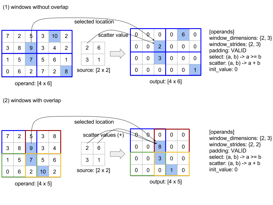
סדר ההערכה של הפונקציה scatter הוא שרירותי, ויכול להיות שהוא לא דטרמיני. לכן הפונקציה scatter לא צריכה להיות רגישה מדי לשיוך מחדש. לפרטים נוספים, כדאי לקרוא את הדיון על אסוציאטיביות בהקשר של Reduce.
שליחה
למידע נוסף: XlaBuilder::Send.
Send(operand, channel_handle)
| ארגומנטים | סוג | סמנטיקה |
|---|---|---|
operand |
XlaOp |
נתונים לשליחה (מערך מסוג T) |
channel_handle |
ChannelHandle |
מזהה ייחודי לכל צמד שליחה/הקלטה |
שליחת נתוני האופרנד הנתונים להוראה Recv בחישוב אחר
שאותו מזהה ערוץ. לא מחזיר נתונים.
בדומה לפעולה Recv, הפעולה של Client API של Send מייצגת תקשורת סינכרונית, ומפרקת אותה באופן פנימי לשתי הוראות HLO (Send ו-SendDone) כדי לאפשר העברות נתונים אסינכרוניות. למידע נוסף: HloInstruction::CreateSend ו-HloInstruction::CreateSendDone.
Send(HloInstruction operand, int64 channel_id)
מופעלת העברה אסינכרונית של האופרנד למשאבים שהוקצו על ידי ההוראה Recv עם אותו מזהה ערוץ. מחזירה הקשר, שמשמש
על ידי הוראת SendDone הבאה, כדי להמתין להשלמת
העברת הנתונים. ההקשר הוא שילוב של {operand (shape), מזהה בקשה (U32)} ואפשר להשתמש בו רק בהוראה של SendDone.
SendDone(HloInstruction context)
בהתאם להקשר שנוצר על ידי הוראה של Send, צריך להמתין להשלמת העברת הנתונים. ההוראה לא מחזירה נתונים כלשהם.
תזמון הוראות לערוצים
סדר הביצוע של 4 ההוראות לכל ערוץ (Recv, RecvDone,
Send, SendDone) מופיע בהמשך.
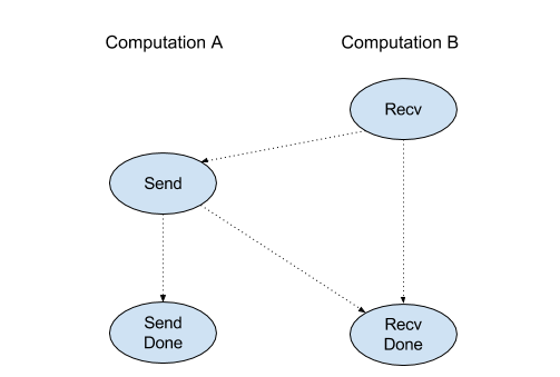
Recvמתרחש לפניSendSendמתרחש לפניRecvDoneRecvמתרחש לפניRecvDoneSendמתרחש לפניSendDone
כשהמהדרים של הקצה העורפי יוצרים לוח זמנים לינארי לכל חישוב שמתקשר באמצעות הוראות ערוצים, לא יכולים להיות מחזורים בין החישובים השונים. לדוגמה: לוחות הזמנים הבאים מובילים למבוי סתום.
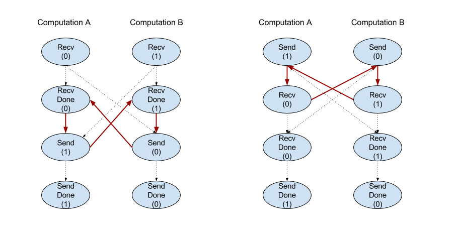
תבנית של תוכן דינמי
למידע נוסף: XlaBuilder::Slice.
חיתוך מחלץ מערך משנה ממערך הקלט. מערך המשנה הוא בעל אותו דירוג כמו הקלט, ומכיל את הערכים בתוך תיבה תוחמת בתוך מערך הקלט, שבה המימדים והאינדקסים של התיבה התוחמת נתונים כארגומנטים לפעולת הפלח.
Slice(operand, start_indices, limit_indices, strides)
| ארגומנטים | סוג | סמנטיקה |
|---|---|---|
operand |
XlaOp |
מערך ממדי N מסוג T |
start_indices |
ArraySlice<int64> |
רשימה של N מספרים שלמים שמכילה את האינדקסים המתחילים של הפלח לכל מאפיין. הערכים צריכים להיות גדולים מ-0 או שווים לו. |
limit_indices |
ArraySlice<int64> |
רשימה של N מספרים שלמים שמכילים את האינדקסים הסופיים (לא כולל) של הפלח של כל מאפיין. כל ערך צריך להיות גדול או שווה לערך של start_indices המתאים למאפיין, וקטן מגודל המאפיין או שווה לו. |
strides |
ArraySlice<int64> |
רשימה של N מספרים שלמים שקובעים את צעד הקלט של הפלח. הפלח בוחר כל רכיב strides[d] במאפיין d. |
דוגמה חד-ממדית:
let a = {0.0, 1.0, 2.0, 3.0, 4.0}
Slice(a, {2}, {4}) produces:
  {2.0, 3.0}
דוגמה דו-ממדית:
let b =
 { {0.0,  1.0,  2.0},
   {3.0,  4.0,  5.0},
   {6.0,  7.0,  8.0},
   {9.0, 10.0, 11.0} }

Slice(b, {2, 1}, {4, 3}) produces:
  { { 7.0,  8.0},
    {10.0, 11.0} }
מיון
למידע נוסף: XlaBuilder::Sort.
Sort(operands, comparator, dimension, is_stable)
| ארגומנטים | סוג | סמנטיקה |
|---|---|---|
operands |
ArraySlice<XlaOp> |
האופרנדים למיון. |
comparator |
XlaComputation |
חישובי המשווה שצריך להשתמש בו. |
dimension |
int64 |
המאפיין שלאורכו יש למיין. |
is_stable |
bool |
האם יש להשתמש במיון יציב. |
אם מספקים רק אופרנד אחד:
אם האופרנד הוא טנזור דרגה 1 (מערך), התוצאה היא מערך ממוין. אם רוצים למיין את המערך בסדר עולה, המשווה צריך לבצע השוואה של 'פחות מ-'. באופן רשמי, אחרי שהמערך ממוין, הוא שמור בכל מיקומי האינדקס
i, jעםi < jשמתחיל ב-comparator(value[i], value[j]) = comparator(value[j], value[i]) = falseאו ב-comparator(value[i], value[j]) = true.אם לאופרנד יש דירוג גבוה יותר, האופרנד ממוין לפי המאפיין שצוין. לדוגמה, עבור Tensor דירוג 2 (מטריצה), ערך המאפיין
0ימיין באופן עצמאי את כל העמודות, וערך המאפיין1ימיין בנפרד כל שורה. אם לא תספקו מספר מאפיין, המאפיין האחרון ייבחר כברירת מחדל. לגבי המאפיין שממוין, חל אותו סדר מיון כמו במקרה של דירוג 1.
אם סופקו אופרנדים n > 1:
כל האופרנדים מסוג
nחייבים להיות טנסים עם אותם מימדים. סוגי הרכיבים של המתנסים עשויים להיות שונים.כל האופרנדים ממוינים יחד, לא בנפרד. באופן כללי, האופרנדים מתייחסים לאופרנדים. כשבודקים אם צריך להחליף את הרכיבים של כל אופרנד במיקומים
iו-j, מתבצעת קריאה למשווה עם2 * nפרמטרים סקלריים, כאשר הפרמטר2 * kתואם לערך במיקוםiמהאופרנדk-th, והפרמטר2 * k + 1תואם לערך שבמיקוםjמהאופרנדk-th. בדרך כלל המשווה משווה בין הפרמטרים2 * kו-2 * k + 1, ויכול להיות שהוא ישתמש בזוגות אחרים של פרמטרים כמעברי קשר.התוצאה היא צירוף שכולל את האופרנדים לפי סדר ממוין (לאורך המאפיין הנתון, כפי שמתואר למעלה). האופרנד
i-thשל ה-tuple תואם לאופרנדi-thשל מיון.
לדוגמה, אם יש שלושה אופרנדים operand0 = [3, 1], operand1 = [42, 50], operand2 = [-3.0, 1.1], והמשווה משווה רק את הערכים של operand0 עם 'פחות מ-', אז הפלט מהסוג הזה הוא ([1, 3], [50, 42], [1.1, -3.0]) ב-tuple.
אם המדיניות is_stable מוגדרת כ-True, המיון יהיה יציב. כלומר, אם יש רכיבים שהמשווה נחשבים כשווים, הסדר היחסי של הערכים השווים יישמר. שני הרכיבים e1 ו-e2
שווה אם ורק אם comparator(e1, e2) = comparator(e2, e1) = false. כברירת מחדל, is_stable מוגדר כ-False.
החלפה
ראו גם את הפעולה tf.reshape.
Transpose(operand)
| ארגומנטים | סוג | סמנטיקה |
|---|---|---|
operand |
XlaOp |
האופרנד שיש להחליף. |
permutation |
ArraySlice<int64> |
איך לשנות את המאפיינים. |
מתאימה את מידות האופרנד בעזרת הפרמוטציה הנתונה, כך
∀ i . 0 ≤ i < rank ⇒ input_dimensions[permutation[i]] = output_dimensions[i].
היא זהה ל-Reshape(אופרנד, פרמוטציה, Permute(permutation, operand.shape.dimensions)).
TriangularSolve
למידע נוסף: XlaBuilder::TriangularSolve.
פתרון מערכות של משוואות ליניאריות עם מטריצות של משולש תחתון או משולש עליון
באמצעות החלפה קדימה או אחורה. שידור לאורך מאפיינים מובילים, התרחיש הזה פותר את אחת ממערכות המטריצה op(a) * x =
b, או x * op(a) = b, עבור המשתנה x, בהינתן a ו-b, כאשר op(a) הוא op(a) = a, או op(a) = Transpose(a), או op(a) = Conj(Transpose(a)).
TriangularSolve(a, b, left_side, lower, unit_diagonal, transpose_a)
| ארגומנטים | סוג | סמנטיקה |
|---|---|---|
a |
XlaOp |
מערך > 2 מסוג מורכב או נקודה צפה (floating-point) עם הצורה [..., M, M]. |
b |
XlaOp |
מערך > 2 מאותו סוג עם הצורה [..., M, K] אם left_side נכון, אחרת [..., K, M]. |
left_side |
bool |
מציין אם לפתור מערכת מהצורה op(a) * x = b (true) או x * op(a) = b (false). |
lower |
bool |
האם להשתמש במשולש העליון או התחתון של a. |
unit_diagonal |
bool |
אם הערך true, האלכסון של a נחשב ל-1 ולא מתבצעת גישה אליו. |
transpose_a |
Transpose |
האם להשתמש ב-a כפי שהוא, לשנות את המיקום שלו או להשתמש במחליפות הצמודות שלו. |
קריאה של נתוני הקלט רק מהמשולש התחתון/העליון של a, בהתאם
לערך של lower. המערכת תתעלם מהערכים מהמשולש השני. נתוני הפלט מוחזרים באותו משולש. הערכים במשולש השני מוגדרים לפי ההטמעה והם יכולים להיות כל דבר.
אם הדירוג של a ו-b גדול מ-2, המערכת מתייחסת אליהן כקבוצות של מטריצות, שבהן כל המאפיינים חוץ מ-2 המאפיינים המינוריים הם מאפייני אצווה. ל-a ול-b צריכות להיות מידות זהות באצווה.
טופל
למידע נוסף: XlaBuilder::Tuple.
צמד (tuple) שמכיל מספר משתנה של נקודות אחיזה לנתונים, ולכל אחת מהן יש צורה משלה.
הדבר דומה ל-std::tuple ב-C++. מבחינה מושגים:
let v: f32[10] = f32[10]{0, 1, 2, 3, 4, 5, 6, 7, 8, 9};
let s: s32 = 5;
let t: (f32[10], s32) = tuple(v, s);
ניתן לבנות את ה-Tples באמצעות הפעולה GetTupleElement.
אף שהפונקציה
למידע נוסף: XlaBuilder::While.
While(condition, body, init)
| ארגומנטים | סוג | סמנטיקה |
|---|---|---|
condition |
XlaComputation |
XlaComputation מסוג T -> PRED המגדיר את תנאי הסיום של theloop. |
body |
XlaComputation |
XlaComputation מסוג T -> T שמגדיר את גוף הלולאה. |
init |
T |
ערך ראשוני לפרמטר condition ו-body. |
מריץ את body ברצף עד שהcondition נכשל. המצב הזה דומה ללולאה אופיינית מסוג לולאת השראה בשפות רבות אחרות, למעט ההבדלים והמגבלות שמפורטים בהמשך.
- צומת
Whileמחזיר ערך מסוגT, שמתקבל מההפעלה האחרונה שלbody. - הצורה של הסוג
Tנקבעת באופן סטטי וחייבת להיות זהה בכל החזרות.
הפרמטרים T של החישובים מתחילים עם הערך init באיטרציה הראשונה, ומתעדכנים באופן אוטומטי לתוצאה החדשה מ-body בכל איטרציה נוספת.
אחד התרחישים לדוגמה העיקרי של הצומת While הוא הטמעה של ביצוע חוזר של אימון ברשתות נוירונים. למטה מוצג פסאודו-קוד מפושט עם גרף שמייצג את החישוב. הקוד נמצא בכתובת while_test.cc.
הסוג T בדוגמה הזו הוא Tuple שמכיל int32 לספירת האיטרציות ו-vector[10] לצובר. ב-1,000 חזרות, הלולאה ממשיכה להוסיף וקטור קבוע למצבר.
// Pseudocode for the computation.
init = {0, zero_vector[10]} // Tuple of int32 and float[10].
result = init;
while (result(0) < 1000) {
  iteration = result(0) + 1;
  new_vector = result(1) + constant_vector[10];
  result = {iteration, new_vector};
}