以下では、XlaBuilder インターフェースで定義されたオペレーションのセマンティクスについて説明します。通常、これらのオペレーションは、xla_data.proto の RPC インターフェースで定義されたオペレーションに 1 対 1 で対応します。
命名法に関する注意事項: XLA で一般化されたデータ型が扱うのは、32 ビット浮動小数点数など、均一な型の要素を保持する N 次元配列です。このドキュメントでは、配列を使用して任意の次元の配列を表します。便宜上、特殊なケースにはより具体的でわかりやすい名前が付けられています。たとえば、ベクトルは 1 次元配列で、行列は 2 次元配列です。
AfterAll
XlaBuilder::AfterAll もご覧ください。
AfterAll は、可変数のトークンを受け取り、単一のトークンを生成します。トークンはプリミティブ型であり、副作用オペレーション間でスレッド化して順序を強制できます。AfterAll は、set オペレーションの後にオペレーションを順序付けるためのトークンの結合として使用できます。
AfterAll(operands)
| 引数 | タイプ | セマンティクス |
|---|---|---|
operands |
XlaOp |
可変長トークンの数 |
AllGather
XlaBuilder::AllGather もご覧ください。
レプリカ間で連結を実行します。
AllGather(operand, all_gather_dim, shard_count, replica_group_ids,
channel_id)
| 引数 | タイプ | セマンティクス |
|---|---|---|
operand
|
XlaOp
|
レプリカ間で連結する配列 |
all_gather_dim |
int64 |
連結ディメンション |
replica_groups
|
int64 のベクトルのベクトル |
連結が行われるグループ |
channel_id
|
省略可 int64
|
モジュール間通信用のオプションのチャネル ID |
replica_groupsは、連結が実行されるレプリカ グループのリストです(現在のレプリカのレプリカ ID は、ReplicaIdを使用して取得できます)。各グループ内のレプリカの順序によって、結果内の入力が配置される順序が決まります。replica_groupsは空にするか(この場合、すべてのレプリカが0からN - 1の順に 1 つのグループに属します)、またはレプリカの数と同じ数の要素を含める必要があります。たとえば、replica_groups = {0, 2}, {1, 3}はレプリカ0と2、および1と3を連結します。shard_countは、各レプリカ グループのサイズです。これは、replica_groupsが空の場合に必要になります。channel_idはモジュール間通信に使用されます。相互に通信できるのは、同じchannel_idを持つall-gatherオペレーションのみです。
出力シェイプは、all_gather_dim を shard_count 倍にした入力シェイプです。たとえば、2 つのレプリカがあり、2 つのレプリカでオペランドの値が [1.0, 2.5] と [3.0, 5.25] である場合、all_gather_dim が 0 であるこの演算からの出力値は両方のレプリカで [1.0, 2.5, 3.0,
5.25] になります。
AllReduce
XlaBuilder::AllReduce もご覧ください。
レプリカ間でカスタム計算を実行します。
AllReduce(operand, computation, replica_group_ids, channel_id)
| 引数 | タイプ | セマンティクス |
|---|---|---|
operand
|
XlaOp
|
レプリカ全体で削減する配列または空でない配列のタプル |
computation |
XlaComputation |
削減計算 |
replica_groups
|
int64 のベクトルのベクトル |
リダクションを行うグループ |
channel_id
|
省略可 int64
|
モジュール間通信用のオプションのチャネル ID |
operandが配列のタプルの場合、タプルの各要素に対して all-reduce が実行されます。replica_groupsは、削減が行われるレプリカグループのリストです(現在のレプリカのレプリカ ID はReplicaIdを使用して取得できます)。replica_groupsは空にするか(この場合、すべてのレプリカは単一のグループに属します)、またはレプリカの数と同じ数の要素を含める必要があります。たとえば、replica_groups = {0, 2}, {1, 3}は、レプリカ0と2と、1と3の間で削減を行います。channel_idはモジュール間通信に使用されます。相互に通信できるのは、同じchannel_idを持つall-reduceオペレーションのみです。
出力シェイプは入力シェイプと同じです。たとえば、2 つのレプリカがあり、2 つのレプリカでオペランドがそれぞれ [1.0, 2.5] と [3.0, 5.25] の値を持っている場合、この演算と総和の出力は両方のレプリカで [4.0, 7.75] になります。入力がタプルの場合、出力もタプルです。
AllReduce の結果を計算するには、各レプリカから 1 つの入力が必要になるため、あるレプリカが別のレプリカよりも AllReduce ノードを複数回実行した場合、前のレプリカは永久に待機します。レプリカはすべて同じプログラムを実行しているため、そのようにする方法はあまり多くありませんが、while ループの条件がインフィードのデータに依存し、入力されたデータが原因で while ループがレプリカ間で何度も繰り返される場合があります。
AllToAll
XlaBuilder::AllToAll もご覧ください。
AllToAll は、すべてのコアからすべてのコアにデータを送信する集合オペレーションです。次の 2 つのフェーズがあります。
- 散布フェーズ。各コアで、オペランドは
split_dimensionsに沿ってsplit_count個のブロックに分割され、ブロックはすべてのコアに分散されます。たとえば、i 番目のブロックは i 番目のコアに送信されます。 - 収集フェーズ。各コアは、受け取ったブロックを
concat_dimensionに沿って連結します。
参加するコアは次の方法で構成できます。
replica_groups: 各 ReplicaGroup には、計算に参加するレプリカ ID のリストが含まれます(現在のレプリカのレプリカ ID は、ReplicaIdを使用して取得できます)。AllToAll は指定された順序でサブグループ内に適用されます。たとえば、replica_groups = { {1,2,3}, {4,5,0} }は、AllToAll がレプリカ{1, 2, 3}内と収集フェーズで適用され、受信したブロックが 1、2、3 の同じ順序で連結されることを意味します。さらに、レプリカ 4、5、0 内に別の AllToAll が適用され、連結順序も 4、5、0 になります。replica_groupsが空の場合、すべてのレプリカが、外観の連結順序で 1 つのグループに属します。
事前準備
split_dimension上のオペランドのディメンション サイズはsplit_countで割り切れます。- オペランドの形状がタプルではありません。
AllToAll(operand, split_dimension, concat_dimension, split_count,
replica_groups)
| 引数 | タイプ | セマンティクス |
|---|---|---|
operand |
XlaOp |
N 次元入力配列 |
split_dimension
|
int64
|
オペランドを分割するディメンションの名前を示す、区間 [0,
n) の値 |
concat_dimension
|
int64
|
分割ブロックが連結されるディメンションの名前を示す、区間 [0,
n) の値 |
split_count
|
int64
|
このオペレーションに参加するコアの数。replica_groups が空の場合、レプリカ数を指定します。それ以外の場合は、各グループのレプリカ数と同じにする必要があります。 |
replica_groups
|
ReplicaGroup ベクトル
|
各グループには、レプリカ ID のリストが含まれています。 |
以下に、Alltoall の例を示します。
XlaBuilder b("alltoall");
auto x = Parameter(&b, 0, ShapeUtil::MakeShape(F32, {4, 16}), "x");
AllToAll(x, /*split_dimension=*/1, /*concat_dimension=*/0, /*split_count=*/4);
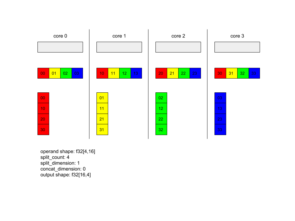
この例では、4 つのコアが Alltoall に参加しています。各コアで、オペランドはディメンション 0 に沿って 4 つの部分に分割されるため、各部分の形状は f32[4,4] になります。4 つの部分がすべてのコアに分散されています。次に、各コアは受け取ったパーツをディメンション 1 に沿って、コア 0 ~ 4 の順序で連結します。したがって、各コアの出力の形状は f32[16,4] です。
BatchNormGrad
アルゴリズムの詳細については、XlaBuilder::BatchNormGrad とバッチ正規化に関する元の論文もご覧ください。
バッチノルムの勾配を計算します。
BatchNormGrad(operand, scale, mean, variance, grad_output, epsilon, feature_index)
| 引数 | タイプ | セマンティクス |
|---|---|---|
operand |
XlaOp |
正規化する n 次元配列(x) |
scale |
XlaOp |
1 次元配列(\(\gamma\)) |
mean |
XlaOp |
1 次元配列(\(\mu\)) |
variance |
XlaOp |
1 次元配列(\(\sigma^2\)) |
grad_output |
XlaOp |
BatchNormTraining(\(\nabla y\))に渡された勾配 |
epsilon |
float |
イプシロンの値(\(\epsilon\)) |
feature_index |
int64 |
operand の特徴ディメンションへのインデックス |
特徴次元の特徴(feature_index は operand の特徴次元のインデックス)ごとに、他のすべての次元の operand、offset、scale に関する勾配を計算します。feature_index は、operand 内の特徴ディメンションに対して有効なインデックスである必要があります。
3 つのグラデーションは、次の式で定義されます(4 次元配列を operand、特徴ディメンション インデックスが l、バッチサイズ m、空間サイズ w と h であると仮定)。
\[ \begin{split} c_l&= \frac{1}{mwh}\sum_{i=1}^m\sum_{j=1}^w\sum_{k=1}^h \left( \nabla y_{ijkl} \frac{x_{ijkl} - \mu_l}{\sigma^2_l+\epsilon} \right) \\\\ d_l&= \frac{1}{mwh}\sum_{i=1}^m\sum_{j=1}^w\sum_{k=1}^h \nabla y_{ijkl} \\\\ \nabla x_{ijkl} &= \frac{\gamma_{l} }{\sqrt{\sigma^2_{l}+\epsilon} } \left( \nabla y_{ijkl} - d_l - c_l (x_{ijkl} - \mu_{l}) \right) \\\\ \nabla \gamma_l &= \sum_{i=1}^m\sum_{j=1}^w\sum_{k=1}^h \left( \nabla y_{ijkl} \frac{x_{ijkl} - \mu_l}{\sqrt{\sigma^2_{l}+\epsilon} } \right) \\\\\ \nabla \beta_l &= \sum_{i=1}^m\sum_{j=1}^w\sum_{k=1}^h \nabla y_{ijkl} \end{split} \]
入力 mean と variance は、バッチディメンションと空間ディメンションにわたるモーメント値を表します。
出力タイプは、次の 3 つのハンドルのタプルです。
| 出力 | タイプ | セマンティクス |
|---|---|---|
grad_operand
|
XlaOp
|
入力 operand($\nabla x$)に関する勾配 |
grad_scale
|
XlaOp
|
入力 scale($\nabla \gamma$)に関する勾配 |
grad_offset
|
XlaOp
|
入力 offset($\nabla \beta$)に関する勾配 |
BatchNormInference
アルゴリズムの詳細については、XlaBuilder::BatchNormInference とバッチ正規化に関する元の論文もご覧ください。
バッチ ディメンションと空間ディメンション全体で配列を正規化します。
BatchNormInference(operand, scale, offset, mean, variance, epsilon, feature_index)
| 引数 | タイプ | セマンティクス |
|---|---|---|
operand |
XlaOp |
正規化する N 次元配列 |
scale |
XlaOp |
1 次元配列 |
offset |
XlaOp |
1 次元配列 |
mean |
XlaOp |
1 次元配列 |
variance |
XlaOp |
1 次元配列 |
epsilon |
float |
イプシロン値 |
feature_index |
int64 |
operand の特徴ディメンションへのインデックス |
特徴ディメンション(feature_index は operand の特徴ディメンションのインデックス)ごとに、他のすべてのディメンションの平均と分散を計算し、平均と分散を使用して operand の各要素を正規化します。feature_index は、operand 内の特徴ディメンションに対して有効なインデックスにする必要があります。
BatchNormInference は、バッチごとに mean と variance を計算せずに BatchNormTraining を呼び出す場合と同等です。代わりに、推定値として入力 mean と variance を使用します。この op の目的は推論のレイテンシを短縮することであるため、BatchNormInference という名前が付けられています。
出力は、入力 operand と同じ形状を持つ N 次元の正規化された配列です。
BatchNormTraining
アルゴリズムの詳細な説明については、XlaBuilder::BatchNormTraining と the original batch normalization paper をご覧ください。
バッチ ディメンションと空間ディメンション全体で配列を正規化します。
BatchNormTraining(operand, scale, offset, epsilon, feature_index)
| 引数 | タイプ | セマンティクス |
|---|---|---|
operand |
XlaOp |
正規化する n 次元配列(x) |
scale |
XlaOp |
1 次元配列(\(\gamma\)) |
offset |
XlaOp |
1 次元配列(\(\beta\)) |
epsilon |
float |
イプシロンの値(\(\epsilon\)) |
feature_index |
int64 |
operand の特徴ディメンションへのインデックス |
特徴ディメンション(feature_index は operand の特徴ディメンションのインデックス)ごとに、他のすべてのディメンションの平均と分散を計算し、平均と分散を使用して operand の各要素を正規化します。feature_index は、operand 内の特徴ディメンションに対して有効なインデックスにする必要があります。
空間次元のサイズとして w と h を持つ m 要素を含む operand \(x\) の各バッチでは、アルゴリズムは次のようになります(operand が 4 次元配列であると仮定します)。
特徴ディメンションの特徴
lごとに \(\mu_l\) バッチ平均を計算します。\(\mu_l=\frac{1}{mwh}\sum_{i=1}^m\sum_{j=1}^w\sum_{k=1}^h x_{ijkl}\)バッチ分散を計算します \(\sigma^2_l\): $\sigma^2l=\frac{1}{mwh}\sum{i=1}^m\sum{j=1}^w\sum{k=1}^h (x_{ijkl} - \mu_l)^2$
正規化、スケーリング、シフト:\(y_{ijkl}=\frac{\gamma_l(x_{ijkl}-\mu_l)}{\sqrt[2]{\sigma^2_l+\epsilon} }+\beta_l\)
イプシロン値(通常は小さな数)は、ゼロ除算エラーを避けるために追加されます。
出力タイプは 3 つの XlaOp のタプルです。
| 出力 | タイプ | セマンティクス |
|---|---|---|
output
|
XlaOp
|
入力 operand(y)と同じ形状の n 次元配列 |
batch_mean |
XlaOp |
1 次元配列(\(\mu\)) |
batch_var |
XlaOp |
1 次元配列(\(\sigma^2\)) |
batch_mean と batch_var は、上記の式を使用してバッチと空間ディメンション全体で計算されたモーメントです。
BitcastConvertType
XlaBuilder::BitcastConvertType もご覧ください。
TensorFlow の tf.bitcast と同様に、データシェイプからターゲット シェイプへの要素単位のビットキャスト オペレーションを実行します。入力サイズと出力サイズが一致している必要があります。たとえば、s32 要素はビットキャスト ルーチンによって f32 要素になり、1 つの s32 要素は 4 つの s8 要素になります。ビットキャストは低レベルのキャストとして実装されるため、異なる浮動小数点表現を持つマシンは異なる結果になります。
BitcastConvertType(operand, new_element_type)
| 引数 | タイプ | セマンティクス |
|---|---|---|
operand |
XlaOp |
ディメンション D を持つ T 型の配列 |
new_element_type |
PrimitiveType |
タイプ U |
オペランドのディメンションとターゲットのシェイプのディメンションは、変換前後のプリミティブ サイズの比率によって変化する最後のディメンションを除き、一致している必要があります。
ソース要素とデスティネーション要素のタイプをタプルにすることはできません。
幅の異なるプリミティブ型へのビットキャスト変換
BitcastConvert HLO 命令は、出力要素型 T' のサイズが入力要素 T のサイズと等しくない場合をサポートします。すべての演算は概念的にはビットキャストであり、基となるバイトを変更しないため、出力要素の形状を変更する必要があります。B = sizeof(T), B' =
sizeof(T') の場合、次の 2 つのケースが考えられます。
まず、B > B' の場合、出力シェイプはサイズ B/B' の新しいマイナー ディメンションを取得します。次に例を示します。
f16[10,2]{1,0} %output = f16[10,2]{1,0} bitcast-convert(f32[10]{0} %input)
有効なスカラーのルールは変わりません。
f16[2]{0} %output = f16[2]{0} bitcast-convert(f32[] %input)
または、B' > B の場合、入力シェイプの最後の論理ディメンションが B'/B と等しくなければならず、このディメンションは変換中に破棄されます。
f32[10]{0} %output = f32[10]{0} bitcast-convert(f16[10,2]{1,0} %input)
異なるビット幅間の変換は要素単位ではないことに注意してください。
ブロードキャスト
XlaBuilder::Broadcast もご覧ください。
配列内のデータを複製して、配列にディメンションを追加します。
Broadcast(operand, broadcast_sizes)
| 引数 | タイプ | セマンティクス |
|---|---|---|
operand |
XlaOp |
複製する配列 |
broadcast_sizes |
ArraySlice<int64> |
新しいディメンションのサイズ |
新しいディメンションが左側に挿入されます。つまり、broadcast_sizes の値が {a0, ..., aN} で、オペランドのシェイプのディメンションが {b0, ..., bM} の場合、出力のシェイプのディメンションは {a0, ..., aN, b0, ..., bM} です。
オペランドのコピーに対する新しいディメンション インデックス。つまり、
output[i0, ..., iN, j0, ..., jM] = operand[j0, ..., jM]
たとえば、operand が値 2.0f を持つスカラー f32 で、broadcast_sizes が {2, 3} の場合、結果はシェイプ f32[2, 3] を持つ配列になり、結果のすべての値は 2.0f になります。
BroadcastInDim
XlaBuilder::BroadcastInDim もご覧ください。
配列内のデータを複製して、配列のサイズとランクを拡張します。
BroadcastInDim(operand, out_dim_size, broadcast_dimensions)
| 引数 | タイプ | セマンティクス |
|---|---|---|
operand |
XlaOp |
複製する配列 |
out_dim_size |
ArraySlice<int64> |
ターゲット シェイプのサイズ |
broadcast_dimensions |
ArraySlice<int64> |
ターゲット シェイプのオペランド シェイプの各次元に対応するディメンション |
Broadcast と似ていますが、任意の場所にディメンションを追加し、サイズ 1 で既存のディメンションを拡張できます。
operand は、out_dim_size で記述されるシェイプにブロードキャストされます。
broadcast_dimensions は、operand のディメンションをターゲット シェイプのディメンションにマッピングします。つまり、オペランドの i ディメンションは、出力シェイプの broadcast_dimension[i] のディメンションにマッピングされます。operand のディメンションは、サイズ 1 にするか、マッピングされる出力シェイプのディメンションと同じサイズにする必要があります。残りのディメンションにはサイズ 1 のディメンションが入力されます。縮退ディメンションのブロードキャストは、これらの縮退ディメンションに沿ってブロードキャストを行い、出力シェイプに達します。セマンティクスの詳細については、ブロードキャストのページをご覧ください。
電話
XlaBuilder::Call もご覧ください。
指定された引数を使用して計算を呼び出します。
Call(computation, args...)
| 引数 | タイプ | セマンティクス |
|---|---|---|
computation |
XlaComputation |
任意の型の N 個のパラメータによる T_0, T_1, ..., T_{N-1} -> S 型の計算 |
args |
N 個の XlaOp のシーケンス |
任意の型の N 個の引数 |
args のアリティと型は computation のパラメータと一致する必要があります。args は設定できません。
コレスキー
XlaBuilder::Cholesky もご覧ください。
対称(エルミート)正定行列のバッチのコレスキー分解を計算します。
Cholesky(a, lower)
| 引数 | タイプ | セマンティクス |
|---|---|---|
a |
XlaOp |
複素数または浮動小数点型の、ランク > 2 の配列。 |
lower |
bool |
a の上向き三角形と下三角形のどちらを使用するかを指定します。 |
lower が true の場合、$a = l となるように下三角行列 l を計算します。
l^T$。lower が false の場合、\(a = u^T . u\)となるように上三角行列 u を計算します。
入力データは、lower の値に応じて、a の下/上向きの三角形からのみ読み取られます。もう一方の三角形の値は無視されます。出力データは同じ三角形に返されます。他方の三角形の値は実装によって定義されるため、何でもかまいません。
a のランクが 2 より大きい場合、a は行列のバッチとして処理されます。ここで、マイナー 2 ディメンションを除くすべてのディメンションがバッチ ディメンションです。
a が対称(エルミート)正定値でない場合、結果は実装で定義されます。
クランプ
XlaBuilder::Clamp もご覧ください。
オペランドを最小値と最大値の間の範囲内に固定します。
Clamp(min, operand, max)
| 引数 | タイプ | セマンティクス |
|---|---|---|
min |
XlaOp |
T 型の配列 |
operand |
XlaOp |
T 型の配列 |
max |
XlaOp |
T 型の配列 |
オペランドと、最小値と最大値が与えられた場合、そのオペランドが最小値と最大値の間の範囲内であれば最小値を返し、そうでない場合はオペランドがこの範囲より低い場合は最小値を返します。この範囲を上回る場合は最大値を返します。つまり、clamp(a, x, b) = min(max(a, x), b) のようになります。
3 つの配列はすべて同じ形状である必要があります。または、ブロードキャストの制限された形式として、min または max を T 型のスカラーにできます。
スカラー min と max を使用した例:
let operand: s32[3] = {-1, 5, 9};
let min: s32 = 0;
let max: s32 = 6;
==>
Clamp(min, operand, max) = s32[3]{0, 5, 6};
閉じる
XlaBuilder::Collapse および tf.reshape オペレーションもご覧ください。
配列の複数のディメンションを 1 つのディメンションに折りたたみます。
Collapse(operand, dimensions)
| 引数 | タイプ | セマンティクス |
|---|---|---|
operand |
XlaOp |
T 型の配列 |
dimensions |
int64 個のベクター |
順番に T のディメンションの連続するサブセットを並べます。 |
fold は、オペランドのディメンションの指定されたサブセットを単一のディメンションに置き換えます。入力引数は、T 型の任意の配列と、ディメンション インデックスのコンパイル時定数ベクトルです。ディメンション インデックスは、T ディメンションの連続するサブセットを順序付き(低次元から高次元まで)する必要があります。したがって、{0, 1, 2}、{0, 1}、{1, 2} はすべて有効なディメンション セットですが、{1, 0} や {0, 2} は有効ではありません。これらは、元のディメンション サイズの積に等しい新しいディメンション サイズで、ディメンション シーケンス内の置き換えられる位置と同じ位置にある 1 つの新しいディメンションに置き換えられます。dimensions のディメンションの最も小さいディメンションは、これらのディメンションを折りたたむループのネストの中で最も変化が遅いディメンション(最もメジャー)であり、最も大きいディメンションの数値は最も変化が最も大きい(最もマイナー)です。より一般的な折りたたみの順序が必要な場合は、tf.reshape 演算子をご覧ください。
たとえば、v を 24 個の要素の配列とします。
let v = f32[4x2x3] { { {10, 11, 12},  {15, 16, 17} },
{ {20, 21, 22},  {25, 26, 27} },
{ {30, 31, 32},  {35, 36, 37} },
{ {40, 41, 42},  {45, 46, 47} } };

// Collapse to a single dimension, leaving one dimension.
let v012 = Collapse(v, {0,1,2});
then v012 == f32[24] {10, 11, 12, 15, 16, 17,
20, 21, 22, 25, 26, 27,
30, 31, 32, 35, 36, 37,
40, 41, 42, 45, 46, 47};

// Collapse the two lower dimensions, leaving two dimensions.
let v01 = Collapse(v, {0,1});
then v01 == f32[4x6] { {10, 11, 12, 15, 16, 17},
{20, 21, 22, 25, 26, 27},
{30, 31, 32, 35, 36, 37},
{40, 41, 42, 45, 46, 47} };

// Collapse the two higher dimensions, leaving two dimensions.
let v12 = Collapse(v, {1,2});
then v12 == f32[8x3] { {10, 11, 12},
{15, 16, 17},
{20, 21, 22},
{25, 26, 27},
{30, 31, 32},
{35, 36, 37},
{40, 41, 42},
{45, 46, 47} };
CollectivePermute
XlaBuilder::CollectivePermute もご覧ください。
CollectivePermute は、レプリカ間でデータを送受信する集団オペレーションです。
CollectivePermute(operand, source_target_pairs)
| 引数 | タイプ | セマンティクス |
|---|---|---|
operand |
XlaOp |
N 次元入力配列 |
source_target_pairs |
<int64, int64> 個のベクター |
source_replica_id、target_replica_id のペアのリスト。ペアごとに、オペランドがソース レプリカからターゲット レプリカに送信されます。 |
source_target_pair には次の制限があります。
- 2 つのペアに同じターゲット レプリカ ID を持たせることはできません。また、ソースレプリカ ID を同じにしないでください。
- レプリカ ID がどのペアのターゲットでもない場合、そのレプリカの出力は入力と同じ形状の 0 で構成されるテンソルになります。
Concatenate
XlaBuilder::ConcatInDim もご覧ください。
連結は、複数の配列オペランドから配列を作成します。配列は、各入力配列オペランドと同じランク(互いに同じランクでなければなりません)であり、引数が指定された順序で含まれます。
Concatenate(operands..., dimension)
| 引数 | タイプ | セマンティクス |
|---|---|---|
operands |
N XlaOp のシーケンス |
T 型の次元が [L0, L1, ...] の配列。N >= 1 でなければなりません。 |
dimension |
int64 |
operands との間に連結されるディメンションの名前を指定する、区間 [0, N) の値。 |
dimension を除き、すべてのディメンションが同じである必要があります。これは、XLA が「不規則な」配列をサポートしていないためです。また、ランク 0 の値は連結できません(連結が行われるディメンションに名前を付けることができないため)。
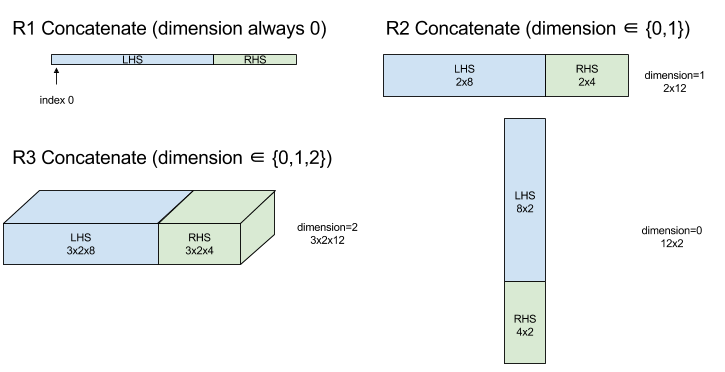
1 次元の例:
Concat({ {2, 3}, {4, 5}, {6, 7} }, 0)
>>> {2, 3, 4, 5, 6, 7}
2 次元の例:
let a = {
{1, 2},
{3, 4},
{5, 6},
};
let b = {
{7, 8},
};
Concat({a, b}, 0)
>>> {
{1, 2},
{3, 4},
{5, 6},
{7, 8},
}
図:
条件
XlaBuilder::Conditional もご覧ください。
Conditional(pred, true_operand, true_computation, false_operand,
false_computation)
| 引数 | タイプ | セマンティクス |
|---|---|---|
pred |
XlaOp |
PRED 型のスカラー |
true_operand |
XlaOp |
\(T_0\)型の引数 |
true_computation |
XlaComputation |
\(T_0 \to S\)型の XlaComputation |
false_operand |
XlaOp |
\(T_1\)型の引数 |
false_computation |
XlaComputation |
\(T_1 \to S\)型の XlaComputation |
pred が true の場合は true_computation、pred が false の場合は false_computation を実行し、結果を返します。
true_computation は、 \(T_0\) 型の引数を 1 つだけ受け取る必要があり、同じ型でなければなりません。true_operand で呼び出されます。false_computation は、 \(T_1\) 型の単一の引数を取る必要があり、同じ型である false_operand で呼び出されます。true_computation と false_computation の戻り値の型は同じである必要があります。
pred の値に応じて、true_computation または false_computation のいずれか 1 つのみが実行されることに注意してください。
Conditional(branch_index, branch_computations, branch_operands)
| 引数 | タイプ | セマンティクス |
|---|---|---|
branch_index |
XlaOp |
S32 型のスカラー |
branch_computations |
N XlaComputation のシーケンス |
\(T_0 \to S , T_1 \to S , ..., T_{N-1} \to S\)型の XlaComputations |
branch_operands |
N XlaOp のシーケンス |
\(T_0 , T_1 , ..., T_{N-1}\)型の引数 |
branch_computations[branch_index] を実行し、結果を返します。branch_index が S32 で、< 0 または >= N の場合、branch_computations[N-1] がデフォルト ブランチとして実行されます。
各 branch_computations[b] は、 \(T_b\) 型の引数を 1 つだけ取る必要があり、同じ型の branch_operands[b] で呼び出されます。各 branch_computations[b] の戻り値の型は同じである必要があります。
branch_index の値に応じて、branch_computations の 1 つのみが実行されることに注意してください。
コンバージョン(畳み込み)
XlaBuilder::Conv もご覧ください。
ConvWithGeneralPadding と同じですが、パディングは簡潔に SAME または VALID として指定されます。同じパディングでは、入力(lhs)にゼロがパディングされます。これにより、ストライディングを考慮しない場合、出力が入力と同じ形状になります。VALID パディングは、単にパディングがないことを意味します。
ConvWithGeneralPadding(畳み込み)
XlaBuilder::ConvWithGeneralPadding もご覧ください。
ニューラル ネットワークで使用される種類の畳み込みを計算します。ここで、畳み込みは、n 次元ベース領域上を移動する n 次元ウィンドウと考えることができ、ウィンドウの考えられる位置ごとに計算が実行されます。
| 引数 | タイプ | セマンティクス |
|---|---|---|
lhs |
XlaOp |
ランク n+2 の入力配列 |
rhs |
XlaOp |
カーネルの重みのランク n+2 の配列 |
window_strides |
ArraySlice<int64> |
カーネル ストライドの N 次元配列 |
padding |
ArraySlice< pair<int64,int64>> |
パディング(低、高)の n 配列 |
lhs_dilation |
ArraySlice<int64> |
n d lhs 拡張係数配列 |
rhs_dilation |
ArraySlice<int64> |
n d rhs 拡張係数の配列 |
feature_group_count |
int64 | 特徴グループの数 |
batch_group_count |
int64 | バッチグループの数 |
n を空間次元の数とします。lhs 引数は、ベース領域を表す n+2 ランクの配列です。これは入力と呼ばれますが、RHS は入力でもあります。ニューラル ネットワークでは、これらは入力の活性化です。n+2 個のディメンションの順序は次のとおりです。
batch: このディメンションの各座標は、畳み込み対象となる独立した入力を表します。z/depth/features: ベース領域内の各 (y,x) 位置には、この次元に入るベクトルが関連付けられています。spatial_dims: ウィンドウが移動するベース領域を定義するn空間ディメンションを記述します。
rhs 引数は、畳み込みフィルタ/カーネル/ウィンドウを記述するランク n+2 の配列です。ディメンションは次の順序で示す。
output-z: 出力のzディメンション。input-z: このディメンションにfeature_group_countを掛けたサイズは、zディメンションのサイズ(L 単位)と等しくなります。spatial_dims: ベース領域上を移動する n-d ウィンドウを定義するn空間次元を記述します。
window_strides 引数は、畳み込みウィンドウのストライドを空間次元で指定します。たとえば、最初の空間次元のストライドが 3 の場合、ウィンドウは最初の空間インデックスが 3 で割り切れる座標にのみ配置できます。
padding 引数は、ベース領域に適用するゼロパディングの量を指定します。パディングの量は負にすることができます。負のパディングの絶対値は、畳み込み処理の前に、指定されたディメンションから削除する要素の数を示します。padding[0] はディメンション y のパディングを指定し、padding[1] はディメンション x のパディングを指定します。各ペアには、最初の要素として低いパディング、2 番目の要素として高いパディングがあります。低いパディングは低いインデックスの方向に適用され、高いパディングは高いインデックスの方向に適用されます。たとえば、padding[1] が (2,3) の場合、2 番目の空間次元には左側に 2 個のゼロ、右側に 3 個のゼロによるパディングがあります。パディングを使用することは、畳み込み処理を行う前に同じゼロ値を入力(lhs)に挿入するのと同じです。
lhs_dilation 引数と rhs_dilation 引数は、各空間次元の lhs と rhs に適用する拡張係数を指定します。空間次元の拡張係数を d とすると、その次元の各エントリの間に暗黙的に d-1 個のホールが配置され、配列のサイズが大きくなります。穴には no-op 値が入っています。これは、畳み込みの場合はゼロを意味します。
右辺の拡張は、アトロス コンボリューションとも呼ばれます。詳しくは、tf.nn.atrous_conv2d をご覧ください。lh の拡散は転置畳み込みとも呼ばれます。詳しくは、tf.nn.conv2d_transpose をご覧ください。
feature_group_count 引数(デフォルト値は 1)は、グループ化された畳み込みに使用できます。feature_group_count は、入力特徴量ディメンションと出力特徴量ディメンションの両方の除数にする必要があります。feature_group_count が 1 より大きい場合、概念的には、入出力特徴ディメンションと rhs 出力特徴ディメンションが多くの feature_group_count グループ(各グループは特徴の連続するサブシーケンスで構成される)に均等に分割されます。rhs の入力特徴ディメンションは、lhs 入力特徴ディメンションを feature_group_count で割った値と同じである必要があります(入力特徴のグループのサイズにすでに含まれているため)。i 番目のグループは、多くの個別の畳み込みの feature_group_count を計算するために一緒に使用されます。これらの畳み込みの結果は、出力特徴ディメンション内で連結されます。
深さ方向の畳み込みの場合、feature_group_count 引数は入力特徴次元に設定され、フィルタの形状は [filter_height, filter_width, in_channels, channel_multiplier] から [filter_height, filter_width, 1, in_channels * channel_multiplier] に変更されます。詳しくは、tf.nn.depthwise_conv2d をご覧ください。
誤差逆伝播法中に、グループ化フィルタに対して batch_group_count(デフォルト値 1)引数を使用できます。batch_group_count は、lhs(入力)バッチ ディメンションのサイズの除数にする必要があります。batch_group_count が 1 より大きい場合、出力バッチ ディメンションは input batch
/ batch_group_count サイズにする必要があります。batch_group_count は、出力特徴サイズの除数にする必要があります。
出力シェイプの寸法は次のとおりです。
batch: このディメンションのサイズにbatch_group_countを掛けた値は、batchディメンションのサイズ(L 単位)と等しくなります。z: カーネル(rhs)のoutput-zと同じサイズ。spatial_dims: 畳み込みウィンドウの有効なプレースメントごとに 1 つの値。

上の図は、batch_group_count フィールドの仕組みを示しています。実質的に、各 1 分のバッチを batch_group_count グループにスライスし、出力特徴についても同じ処理をします。次に、これらのグループごとにペアワイズ畳み込みを行い、出力特徴ディメンションに沿って出力を連結します。他のすべてのディメンション(特徴と空間)のオペレーション セマンティクスは、すべて同じです。
畳み込みウィンドウの有効な配置は、ストライドと、パディング後のベース領域のサイズによって決まります。
畳み込み処理の動作を説明するには、2 次元の畳み込みについて考え、出力で batch、z、y、x の固定座標を選択します。(y,x) は、ベース領域内のウィンドウの角の位置です(空間次元の解釈方法によっては左上隅など)。これで、ベース領域から取得された 2d ウィンドウが作成され、各 2d 点が 1d ベクトルに関連付けられているため、3d ボックスになります。畳み込みカーネルでは、出力座標 z を固定したため、3D ボックスもあります。2 つのボックスの寸法は同じであるため、2 つのボックス間の要素単位の積の合計を取得できます(ドット積と同様)。これが出力値です。
なお、output-z が例の場合、5 に設定すると、ウィンドウの各位置から、出力の z ディメンションに 5 つの値が生成されます。これらの値は、畳み込みカーネルのどの部分を使用するかが異なります。つまり、output-z 座標ごとに値の 3D ボックスが個別に使用されます。したがって、それぞれ異なるフィルタを使用した 5 つの個別の畳み込みと考えることができます。
パディングとストライディングを行う 2 次元畳み込みの擬似コードは次のとおりです。
for (b, oz, oy, ox) {  // output coordinates
  value = 0;
  for (iz, ky, kx) {  // kernel coordinates and input z
    iy = oy*stride_y + ky - pad_low_y;
    ix = ox*stride_x + kx - pad_low_x;
    if ((iy, ix) inside the base area considered without padding) {
      value += input(b, iz, iy, ix) * kernel(oz, iz, ky, kx);
    }
  }
  output(b, oz, oy, ox) = value;
}
ConvertElementType
XlaBuilder::ConvertElementType もご覧ください。
C++ の要素単位の static_cast と同様に、データシェイプからターゲット シェイプへの要素単位の変換オペレーションを実行します。ディメンションが一致する必要があり、変換は要素単位です。たとえば、s32 要素は、s32 から f32 への変換ルーチンによって f32 要素になります。
ConvertElementType(operand, new_element_type)
| 引数 | タイプ | セマンティクス |
|---|---|---|
operand |
XlaOp |
ディメンション D を持つ T 型の配列 |
new_element_type |
PrimitiveType |
タイプ U |
オペランドのディメンションとターゲットのシェイプは一致している必要があります。ソース要素とデスティネーション要素のタイプは、タプルにしないでください。
T=s32 から U=f32 への変換では、正規化された int から浮動小数点への変換ルーチン(例: round-nearest-even など)が実行されます。
let a: s32[3] = {0, 1, 2};
let b: f32[3] = convert(a, f32);
then b == f32[3]{0.0, 1.0, 2.0}
CrossReplicaSum
AllReduce と総和計算を実行します。
CustomCall
XlaBuilder::CustomCall もご覧ください。
計算内でユーザー提供の関数を呼び出します。
CustomCall(target_name, args..., shape)
| 引数 | タイプ | セマンティクス |
|---|---|---|
target_name |
string |
関数の名前。このシンボル名をターゲットとする呼び出し命令が生成されます。 |
args |
N 個の XlaOp のシーケンス |
任意の型の N 個の引数。関数に渡されます。 |
shape |
Shape |
関数の出力シェイプ |
引数のアリティや型に関係なく、関数のシグネチャは同じです。
extern "C" void target_name(void* out, void** in);
たとえば、CustomCall が次のように使用されているとします。
let x = f32[2] {1,2};
let y = f32[2x3] { {10, 20, 30}, {40, 50, 60} };

CustomCall("myfunc", {x, y}, f32[3x3])
myfunc の実装例を次に示します。
extern "C" void myfunc(void* out, void** in) {
  float (&x)[2] = *static_cast<float(*)[2]>(in[0]);
  float (&y)[2][3] = *static_cast<float(*)[2][3]>(in[1]);
  EXPECT_EQ(1, x[0]);
  EXPECT_EQ(2, x[1]);
  EXPECT_EQ(10, y[0][0]);
  EXPECT_EQ(20, y[0][1]);
  EXPECT_EQ(30, y[0][2]);
  EXPECT_EQ(40, y[1][0]);
  EXPECT_EQ(50, y[1][1]);
  EXPECT_EQ(60, y[1][2]);
  float (&z)[3][3] = *static_cast<float(*)[3][3]>(out);
  z[0][0] = x[1] + y[1][0];
  // ...
}
ユーザー提供の関数に副作用があってはなりません。また、その実行はべき等でなければなりません。
Dot
XlaBuilder::Dot もご覧ください。
Dot(lhs, rhs)
| 引数 | タイプ | セマンティクス |
|---|---|---|
lhs |
XlaOp |
T 型の配列 |
rhs |
XlaOp |
T 型の配列 |
この演算の正確なセマンティクスは、オペランドのランクによって異なります。
| 入力 | 出力 | セマンティクス |
|---|---|---|
ベクトル [n] dot ベクトル [n] |
スカラー | ベクトルドット積 |
行列 [m x k] dot ベクトル [k] |
ベクトル [m] | 行列ベクトル乗算 |
行列 [m x k] dot 行列 [k x n] |
行列 [m x n] | 行列と行列の乗算 |
この演算では、lhs の 2 番目のディメンション(ランク 1 の場合は最初のディメンション)と rhs の最初のディメンションに対する積の合計を実行します。これらは「契約」ディメンションです。lhs と rhs の契約サイズは同じサイズにする必要があります。実際には、ベクトル間のドット積、ベクトル/行列の乗算、行列/行列の乗算に使用できます。
DotGeneral
XlaBuilder::DotGeneral もご覧ください。
DotGeneral(lhs, rhs, dimension_numbers)
| 引数 | タイプ | セマンティクス |
|---|---|---|
lhs |
XlaOp |
T 型の配列 |
rhs |
XlaOp |
T 型の配列 |
dimension_numbers |
DotDimensionNumbers |
圧縮やバッチのディメンションの数値を |
Dot と似ていますが、lhs と rhs の両方に圧縮とバッチのディメンション番号を指定できます。
| DotDimensionNumbers フィールド | タイプ | セマンティクス |
|---|---|---|
lhs_contracting_dimensions
|
int64 の繰り返し | lhs 契約寸法番号 |
rhs_contracting_dimensions
|
int64 の繰り返し | rhs 契約寸法番号 |
lhs_batch_dimensions
|
int64 の繰り返し | lhs 個のバッチ ディメンション番号 |
rhs_batch_dimensions
|
int64 の繰り返し | rhs 個のバッチ ディメンション番号 |
DotGeneral は、dimension_numbers で指定された縮小寸法に対して商品の合計を計算します。
lhs と rhs の関連する契約寸法番号が同じである必要はありませんが、同じ寸法サイズである必要があります。
寸法番号を縮小する例:
lhs = { {1.0, 2.0, 3.0},
{4.0, 5.0, 6.0} }

rhs = { {1.0, 1.0, 1.0},
{2.0, 2.0, 2.0} }

DotDimensionNumbers dnums;
dnums.add_lhs_contracting_dimensions(1);
dnums.add_rhs_contracting_dimensions(1);

DotGeneral(lhs, rhs, dnums) -> { {6.0, 12.0},
{15.0, 30.0} }
lhs と rhs から関連するバッチ ディメンション番号は、同じディメンション サイズである必要があります。
バッチ ディメンション番号を使用した例(バッチサイズ 2、2×2 行列):
lhs = { { {1.0, 2.0},
{3.0, 4.0} },
{ {5.0, 6.0},
{7.0, 8.0} } }

rhs = { { {1.0, 0.0},
{0.0, 1.0} },
{ {1.0, 0.0},
{0.0, 1.0} } }

DotDimensionNumbers dnums;
dnums.add_lhs_contracting_dimensions(2);
dnums.add_rhs_contracting_dimensions(1);
dnums.add_lhs_batch_dimensions(0);
dnums.add_rhs_batch_dimensions(0);

DotGeneral(lhs, rhs, dnums) -> { { {1.0, 2.0},
{3.0, 4.0} },
{ {5.0, 6.0},
{7.0, 8.0} } }
| 入力 | 出力 | セマンティクス |
|---|---|---|
[b0, m, k] dot [b0, k, n] |
[b0, m, n] | バッチ MaMul |
[b0, b1, m, k] dot [b0, b1, k, n] |
[b0, b1, m, n] | バッチ MaMul |
結果として、結果のディメンション番号は、バッチ ディメンションから始まり、次に lhs 非コントラクト/非バッチ ディメンション、最後に rhs 非コントラクト/非バッチ ディメンションから始まります。
DynamicSlice
XlaBuilder::DynamicSlice もご覧ください。
DynamicSlice は、動的な start_indices の入力配列からサブ配列を抽出します。各ディメンションのスライスのサイズは size_indices で渡され、各ディメンションのスライスの排他的区間の終了点([start, start + size])を指定します。start_indices のシェイプはランク 1 で、ディメンション サイズは operand のランクにする必要があります。
DynamicSlice(operand, start_indices, size_indices)
| 引数 | タイプ | セマンティクス |
|---|---|---|
operand |
XlaOp |
T 型の N 次元配列 |
start_indices |
N XlaOp のシーケンス |
各次元のスライスの開始インデックスを含む N 個のスカラー整数のリスト。0 以上の値を指定してください。 |
size_indices |
ArraySlice<int64> |
各ディメンションのスライスサイズを含む N 個の整数のリスト。モジュロ ディメンションのサイズがラップされないように、各値は厳密に 0 より大きく、start + size はディメンションのサイズ以下にする必要があります。 |
有効なスライス インデックスは、スライスを実行する前に、[1, N) のインデックス i ごとに次の変換を適用して計算されます。
start_indices[i] = clamp(start_indices[i], 0, operand.dimension_size[i] - size_indices[i])
これにより、抽出されたスライスは常にオペランド配列に対して境界内に収まるようになります。変換が適用される前にスライスが境界内にあった場合、変換による影響はありません。
1 次元の例:
let a = {0.0, 1.0, 2.0, 3.0, 4.0}
let s = {2}

DynamicSlice(a, s, {2}) produces:
{2.0, 3.0}
2 次元の例:
let b =
{ {0.0,  1.0,  2.0},
{3.0,  4.0,  5.0},
{6.0,  7.0,  8.0},
{9.0, 10.0, 11.0} }
let s = {2, 1}

DynamicSlice(b, s, {2, 2}) produces:
{ { 7.0,  8.0},
{10.0, 11.0} }
DynamicUpdateSlice
XlaBuilder::DynamicUpdateSlice もご覧ください。
DynamicUpdateSlice は、入力配列 operand の値である結果を生成します。スライス update は start_indices で上書きされます。update の形状によって、更新される結果のサブ配列の形状が決まります。
start_indices のシェイプはランク 1 とし、ディメンション サイズは operand のランクにする必要があります。
DynamicUpdateSlice(operand, update, start_indices)
| 引数 | タイプ | セマンティクス |
|---|---|---|
operand |
XlaOp |
T 型の N 次元配列 |
update |
XlaOp |
スライスの更新を含む T 型の N 次元配列。境界外の更新インデックスが生成されないように、更新シェイプの各次元は厳密に 0 より大きく、start + update は各次元のオペランド サイズ以下である必要があります。 |
start_indices |
N XlaOp のシーケンス |
各次元のスライスの開始インデックスを含む N 個のスカラー整数のリスト。0 以上の値を指定してください。 |
有効なスライス インデックスは、スライスを実行する前に、[1, N) のインデックス i ごとに次の変換を適用して計算されます。
start_indices[i] = clamp(start_indices[i], 0, operand.dimension_size[i] - update.dimension_size[i])
これにより、更新されたスライスが常にオペランド配列の範囲内にあることが保証されます。変換が適用される前にスライスが境界内にあった場合、変換による影響はありません。
1 次元の例:
let a = {0.0, 1.0, 2.0, 3.0, 4.0}
let u = {5.0, 6.0}
let s = {2}

DynamicUpdateSlice(a, u, s) produces:
{0.0, 1.0, 5.0, 6.0, 4.0}
2 次元の例:
let b =
{ {0.0,  1.0,  2.0},
{3.0,  4.0,  5.0},
{6.0,  7.0,  8.0},
{9.0, 10.0, 11.0} }
let u =
{ {12.0,  13.0},
{14.0,  15.0},
{16.0,  17.0} }

let s = {1, 1}

DynamicUpdateSlice(b, u, s) produces:
{ {0.0,  1.0,  2.0},
{3.0, 12.0, 13.0},
{6.0, 14.0, 15.0},
{9.0, 16.0, 17.0} }
要素ごとのバイナリ算術演算
XlaBuilder::Add もご覧ください。
一連の要素単位のバイナリ算術演算がサポートされています。
Op(lhs, rhs)
ここで、Op は Add(加算)、Sub(減算)、Mul(乗算)、Div(除算)、Rem(除算)、Max(最大値)、Min(最小)、LogicalAnd(論理 AND)、LogicalOr(論理 OR)のいずれかです。
| 引数 | タイプ | セマンティクス |
|---|---|---|
lhs |
XlaOp |
左側のオペランド: T 型の配列 |
rhs |
XlaOp |
右側のオペランド: T 型の配列 |
引数の形状は類似しているか、互換性がある必要があります。シェイプの互換性の意味については、ブロードキャストのドキュメントをご覧ください。演算の結果のシェイプは、2 つの入力配列をブロードキャストした結果です。このバリアントでは、オペランドの 1 つがスカラーでない限り、異なるランクの配列間の演算はサポートされません。
Op が Rem の場合、被除数から結果の符号が取得され、結果の絶対値は常に除数の絶対値より小さくなります。
整数除算オーバーフロー(ゼロによる符号付き/符号なし除算/余り、または -1 による INT_SMIN の符号付き除算/余り)は、実装で定義された値を生成します。
次のオペレーションに対しては、異なるランクのブロードキャストをサポートする代替バリアントが存在します。
Op(lhs, rhs, broadcast_dimensions)
ここで、Op は上記と同じです。この演算のバリアントは、異なるランクの配列間の算術演算(ベクトルに行列を追加するなど)に使用します。
追加の broadcast_dimensions オペランドは、低ランク オペランドのランクを高ランク オペランドのランクに拡張するために使用される整数のスライスです。broadcast_dimensions は、下位のシェイプのディメンションを上位シェイプのディメンションにマッピングします。展開されたシェイプのマッピングされていないディメンションには、サイズ 1 のディメンションが入力されます。縮退次元ブロードキャストでは、これらの縮退次元に沿ってシェイプをブロードキャストし、両方のオペランドの形状を等しくします。セマンティクスの詳細については、ブロードキャストのページをご覧ください。
要素単位の比較演算
XlaBuilder::Eq もご覧ください。
標準的な要素単位のバイナリ比較演算のセットがサポートされています。なお、浮動小数点型を比較する際は、標準の IEEE 754 浮動小数点比較セマンティクスが適用されます。
Op(lhs, rhs)
ここで、Op は、Eq(等しい)、Ne(等しくない)、Ge(大なりイコール)、Gt(大なりイコール)、Le(不等号)、Lt(小なり)のいずれかです。EqTotalOrder、NeTotalOrder、GeTotalOrder、GtTotalOrder、LeTotalOrder、LtTotalOrder の演算子セットは、同じ機能を提供しますが、-NaN < -Inf < -Finite < -0 < +0 < +Finite < +Finite < N
| 引数 | タイプ | セマンティクス |
|---|---|---|
lhs |
XlaOp |
左側のオペランド: T 型の配列 |
rhs |
XlaOp |
右側のオペランド: T 型の配列 |
引数の形状は類似しているか、互換性がある必要があります。シェイプの互換性の意味については、ブロードキャストのドキュメントをご覧ください。演算の結果のシェイプは、要素型 PRED を持つ 2 つの入力配列をブロードキャストした結果です。このバリアントでは、オペランドの 1 つがスカラーでない限り、異なるランクの配列間の演算はサポートされません。
次のオペレーションに対しては、異なるランクのブロードキャストをサポートする代替バリアントが存在します。
Op(lhs, rhs, broadcast_dimensions)
ここで、Op は上記と同じです。この演算のバリアントは、異なるランクの配列間の比較演算(ベクトルに行列を追加するなど)に使用します。
追加の broadcast_dimensions オペランドは、オペランドのブロードキャストに使用するディメンションを指定する整数のスライスです。セマンティクスの詳細については、ブロードキャストのページをご覧ください。
要素単位の単項関数
XlaBuilder は、次の要素単位の単項関数をサポートしています。
Abs(operand) 要素ごとの絶対値 x -> |x|。
Ceil(operand) 要素単位のセル x -> ⌈x⌉。
Cos(operand) 要素ごとのコサイン x -> cos(x)。
Exp(operand) 要素ごとの自然指数の x -> e^x。
Floor(operand) 要素単位の下限 x -> ⌊x⌋。
Imag(operand) 複雑な(または実数)図形の要素単位の虚数部分。x -> imag(x)。オペランドが浮動小数点型の場合、0 を返します。
IsFinite(operand) operand の各要素が有限(つまり、正の無限大でも負の無限大でもなく、NaN でもない)であるかどうかをテストします。対応する入力要素が有限である場合にのみ、入力と同じ形状の PRED 値の配列を返します。各要素は true です。
Log(operand) 要素ごとの自然対数 x -> ln(x) です。
LogicalNot(operand) x -> !(x) ではなく、要素ごとの論理値です。
Logistic(operand) 要素単位のロジスティック関数の計算 x ->
logistic(x) です。
PopulationCount(operand): operand の各要素に設定されているビット数を計算します。
Neg(operand) 要素ごとの否定の x -> -x。
Real(operand) 複雑な(または実際の)シェイプの要素ごとの実部。
x -> real(x)。オペランドが浮動小数点型の場合、同じ値を返します。
Rsqrt(operand) 平方根演算の要素ごとの逆数 x -> 1.0 / sqrt(x)。
Sign(operand) 要素ごとの符号演算を x -> sgn(x) します。ここで、
\[\text{sgn}(x) = \begin{cases} -1 & x < 0\\ -0 & x = -0\\ NaN & x = NaN\\ +0 & x = +0\\ 1 & x > 0 \end{cases}\]
operand の要素タイプの比較演算子を使用する。
Sqrt(operand) 要素単位の平方根演算の x -> sqrt(x) です。
Cbrt(operand) 要素単位の立方根演算の x -> cbrt(x)。
Tanh(operand) 要素ごとの双曲線正接 x -> tanh(x)。
Round(operand) 要素ごとの丸め(ゼロから近い値)
RoundNearestEven(operand) 要素ごとの丸め、最も近い偶数との相関関係。
| 引数 | タイプ | セマンティクス |
|---|---|---|
operand |
XlaOp |
関数のオペランド |
この関数は、operand 配列内の各要素に適用され、同じ形状の配列になります。operand はスカラー(ランク 0)にできます。
フィート
XLA FFT 演算では、実数および複雑な入出力に対して前方および逆フーリエ変換を実装します。最大 3 軸の多次元 FFT がサポートされています。
XlaBuilder::Fft もご覧ください。
| 引数 | タイプ | セマンティクス |
|---|---|---|
operand |
XlaOp |
フーリエ変換する配列。 |
fft_type |
FftType |
下の表をご覧ください。 |
fft_length |
ArraySlice<int64> |
変換される軸の時間ドメイン長。RFFT(fft_length=[16]) の出力シェイプは RFFT(fft_length=[17]) と同じであるため、これは特に IRFFT で最も内側の軸のサイズを適正化するために必要です。 |
FftType |
セマンティクス |
|---|---|
FFT |
複素数から複素数への FFT を転送する。シェイプは変わりません。 |
IFFT |
複素数から複素数への逆 FFT を実行します。シェイプは変わりません。 |
RFFT |
実数から複雑な FFT への転送を行います。fft_length[-1] がゼロ以外の値の場合、最も内側の軸の形状は fft_length[-1] // 2 + 1 に縮小され、ナイキスト周波数を超える変換済み信号の逆共役部分は省略されます。 |
IRFFT |
逆の実数から複素数の FFT(複素数を取り、実数を返します)。fft_length[-1] がゼロ以外の値の場合、最も内側の軸の形状が fft_length[-1] まで展開され、変換された信号のナイキスト周波数以外の部分が 1 エントリの逆共役から fft_length[-1] // 2 + 1 エントリに推測されます。 |
多次元 FFT
複数の fft_length が指定されている場合、これは最も内側の軸のそれぞれに FFT 演算のカスケードを適用するのと同等です。実数 - 複雑数 - 実数 - 実数の場合、最も内側の軸の変換が(実際には)最初に(RFFT、IRFFT の場合は最後)実行されます。そのため、最も内側の軸でサイズが変わる軸が変化します。他の軸の変換は複雑から複雑になります。
実装の詳細
CPU FFT は、Eigen の TensorFFT を基盤としています。GPU FFT は cuFFT を使用します。
収集
XLA 収集オペレーションは、入力配列の複数のスライス(異なるランタイム オフセットにある各スライス)をつなぎ合わせます。
一般的なセマンティクス
XlaBuilder::Gather もご覧ください。より直感的な説明については、下記の「非公式な説明」をご覧ください。
gather(operand, start_indices, offset_dims, collapsed_slice_dims, slice_sizes, start_index_map)
| 引数 | タイプ | セマンティクス |
|---|---|---|
operand |
XlaOp |
収集元の配列。 |
start_indices |
XlaOp |
収集したスライスの開始インデックスを含む配列。 |
index_vector_dim |
int64 |
開始インデックスを「含む」start_indices のディメンション。詳しくは以下をご覧ください。 |
offset_dims |
ArraySlice<int64> |
オペランドからスライスした配列にオフセットする出力シェイプのディメンションのセット。 |
slice_sizes |
ArraySlice<int64> |
slice_sizes[i] は、ディメンション i のスライスの境界です。 |
collapsed_slice_dims |
ArraySlice<int64> |
折りたたまれた各スライスのディメンションのセット。これらのディメンションはサイズ 1 である必要があります。 |
start_index_map |
ArraySlice<int64> |
start_indices のインデックスをリーガル インデックスにオペランドにマッピングする方法を記述するマップ。 |
indices_are_sorted |
bool |
インデックスが呼び出し元によって確実に並べ替えられるかどうか。 |
unique_indices |
bool |
インデックスが呼び出し元によって一意であることが保証されているかどうか。 |
便宜上、offset_dims ではなく出力配列のディメンションに batch_dims というラベルを付けます。
出力はランク batch_dims.size + offset_dims.size の配列です。
operand.rank は、offset_dims.size と collapsed_slice_dims.size の合計と等しくなる必要があります。また、slice_sizes.size が operand.rank と等しくなる必要があります。
index_vector_dim が start_indices.rank と等しい場合、start_indices には末尾の 1 ディメンションがあると見なされます(つまり、start_indices の形状が [6,7] で、index_vector_dim が 2 の場合、start_indices の形状は暗黙的に [6,7,1] であるとみなします)。
ディメンション i に沿った出力配列の境界は、次のように計算されます。
iがbatch_dimsに存在する(一部のkでbatch_dims[k]に等しい)場合、start_indices.shapeから対応するディメンションの境界が選択され、index_vector_dimはスキップされます(k<index_vector_dimの場合はstart_indices.shape.dims[k]、そうでない場合はstart_indices.shape.dims[k+1] が選択されます)。iがoffset_dimsに存在する(一部のkでoffset_dims[k] に等しい)場合、collapsed_slice_dimsを考慮したうえで、slice_sizesから対応する境界を選択します(adjusted_slice_sizes[k] を選択し、adjusted_slice_sizesはslice_sizesであり、インデックスcollapsed_slice_dimsの境界は除去されます)。
特定の出力インデックス Out に対応するオペランド インデックス In は、正式に次のように計算されます。
G= {Out[k] forbatch_dimsink} とします。Gを使用して、S[i] =start_indices[ combine(G,i)] となるようにベクトルSをスライスします。ここで、 combine(A, b) は位置index_vector_dimの b を A に挿入します。これは、Gが空であっても適切に定義されています。Gが空の場合、S=start_indicesとなります。start_index_mapを使用してSを分散させることで、Sを使用して開始インデックスSinをoperandに作成します。より正確に言うと、Sin[start_index_map[k]] =S[k]:k<start_index_map.sizeの場合。Sin[_] =0。
collapsed_slice_dimsのセットに従ってOutのオフセット ディメンションでインデックスを分散させて、operandに対するインデックスOinを作成します。より正確に言うと、Oin[remapped_offset_dims(k)] =Out[offset_dims[k]]:k<offset_dims.sizeの場合(remapped_offset_dimsは以下で定義)。Oin[_] =0。
InはOin+Sinです。「+」は要素単位の加算です。
remapped_offset_dims は、ドメイン [0, offset_dims.size) と範囲 [0, operand.rank) \ collapsed_slice_dims を持つ単調関数です。たとえばoffset_dims.size は 4、operand.rank は 6、collapsed_slice_dims は {0、2}、remapped_offset_dims は {0→1、
1→3、2→4、3→5} です。
indices_are_sorted が true に設定されている場合、XLA は start_indices がユーザーによって(start_index_map の昇順で)並べ替えられていると想定できます。含まれていない場合、セマンティクスは実装が定義されています。
unique_indices が true に設定されている場合、XLA は分散したすべての要素が一意であると想定できます。そのため、XLA では非アトミック演算を使用できます。unique_indices が true に設定され、分散されているインデックスが一意でない場合、セマンティクスは実装が定義されています。
非公式の説明と例
非公式には、出力配列のすべてのインデックス Out は、次のように計算されるオペランド配列の要素 E に対応します。
Outのバッチ ディメンションを使用して、start_indicesから開始インデックスを検索します。start_index_mapを使用して、開始インデックス(operand.rank より小さい場合もある)をoperandの「full」開始インデックスにマッピングします。完全な開始インデックスを使用して、サイズ
slice_sizesのスライスを動的にスライスします。スライスの形状を変更するには、
collapsed_slice_dimsディメンションを折りたたみます。折りたたみスライスのサイズはすべて、境界 1 でなければならないため、この形状変更は常に有効です。Outのオフセット ディメンションを使用してこのスライスにインデックスを付け、出力インデックスOutに対応する入力要素Eを取得します。
以下のすべての例で、index_vector_dim は start_indices.rank(1)に設定されています。index_vector_dim に値を設定しても演算は根本的に変わりませんが、視覚的表現が煩雑になります。
上記のすべてがいかに組み合わされているかを直感的に理解するため、[16,11] 配列からシェイプ [8,6] の 5 つのスライスを収集する例を見てみましょう。[16,11] 配列内のスライスの位置は、形状 S64[2] のインデックス ベクトルとして表すことができるため、5 つの位置のセットは S64[5,2] 配列として表すことができます。
収集オペレーションの動作は、出力シェイプのインデックスである [G、O0、O1] を取り、次のように入力配列の要素にマッピングするインデックス変換として示すことができます。

まず、G を使用して、収集インデックス配列から(X、Y)ベクトルを選択します。インデックス [G、O0、O1] の出力配列の要素は、インデックス [X+O0,Y+O1] の入力配列の要素です。
slice_sizes は [8,6] で、O0 と O1 の範囲が決まり、これがスライスの境界を決定します。
この収集オペレーションは、G をバッチ ディメンションとするバッチ動的スライスとして機能します。
収集インデックスは多次元である可能性があります。たとえば、上記の例のより一般的なバージョンで形状 [4,5,2] の「gather indices」配列を使用すると、次のようなインデックスが変換されます。

ここでも、バッチ動的スライスの G0 と、バッチ ディメンションの G1 として機能します。スライスのサイズは [8,6] のままです。
XLA の収集オペレーションは、前述の非公式なセマンティクスを次のように一般化します。
出力シェイプのどのディメンションがオフセット ディメンション(最後の例では
O0、O1を含むディメンション)になるかを設定できます。出力のバッチ ディメンション(最後の例ではG0、G1を含むディメンション)は、オフセット ディメンションではない出力ディメンションとして定義されます。出力シェイプに明示的に存在する出力オフセット次元の数は、入力ランクよりも少なくすることもできます。こうした「欠落している」ディメンションは
collapsed_slice_dimsとして明示的にリストされ、スライスサイズを1にする必要があります。これらのメソッドのスライスサイズは1であるため、有効なインデックスは0のみです。これを省略してもあいまいさは生じません。「Collect Indices」配列(最後の例では
X、Y)から抽出されたスライスの要素は、入力配列のランクよりも少ない可能性があります。明示的なマッピングは、入力と同じランクにインデックスを拡張する方法を決定します。
最後の例として、(2)と(3)を使用して tf.gather_nd を実装します。

G0 と G1 は、通常どおりに収集インデックス配列から開始インデックスをスライスするために使用されます。ただし、開始インデックスには要素 X が 1 つだけあります。同様に、値が O0 である出力オフセット インデックスは 1 つだけです。ただし、入力配列のインデックスとして使用される前に、これらは「一連のインデックス マッピング」(正式な説明の start_index_map)と「オフセット マッピング」(正式な説明の remapped_offset_dims)に従って展開され、それぞれ [X,0] と [0、O0] に展開され、[XG1GOG1GOG0O0]01 にセマンティック インデックス [0G1GOG0O0]01 にセマンティックGatherIndicestf.gather_nd
このケースの slice_sizes は [1,11] です。これは直感的に、収集インデックス配列のすべてのインデックス X が行全体を選択することを意味します。結果は、これらのすべての行を連結したものです。
GetDimensionSize
XlaBuilder::GetDimensionSize もご覧ください。
オペランドに指定されたディメンションのサイズを返します。オペランドは配列形式にする必要があります。
GetDimensionSize(operand, dimension)
| 引数 | タイプ | セマンティクス |
|---|---|---|
operand |
XlaOp |
N 次元入力配列 |
dimension |
int64 |
ディメンションを指定する、[0, n) 区間の値 |
SetDimensionSize
XlaBuilder::SetDimensionSize もご覧ください。
XlaOp の指定されたディメンションの動的サイズを設定します。オペランドは配列形式にする必要があります。
SetDimensionSize(operand, size, dimension)
| 引数 | タイプ | セマンティクス |
|---|---|---|
operand |
XlaOp |
N 次元の入力配列。 |
size |
XlaOp |
ランタイムの動的サイズを表す int32。 |
dimension |
int64 |
ディメンションを指定する、[0, n) 区間の値。 |
その結果、コンパイラによって追跡される動的ディメンションを使用して、オペランドを渡します。
パディングされた値は、ダウンストリームのリダクション オペレーションでは無視されます。
let v: f32[10] = f32[10]{1, 2, 3, 4, 5, 6, 7, 8, 9, 10};
let five: s32 = 5;
let six: s32 = 6;

// Setting dynamic dimension size doesn't change the upper bound of the static
// shape.
let padded_v_five: f32[10] = set_dimension_size(v, five, /*dimension=*/0);
let padded_v_six: f32[10] = set_dimension_size(v, six, /*dimension=*/0);

// sum == 1 + 2 + 3 + 4 + 5
let sum:f32[] = reduce_sum(padded_v_five);
// product == 1 * 2 * 3 * 4 * 5
let product:f32[] = reduce_product(padded_v_five);

// Changing padding size will yield different result.
// sum == 1 + 2 + 3 + 4 + 5 + 6
let sum:f32[] = reduce_sum(padded_v_six);
GetTupleElement
XlaBuilder::GetTupleElement もご覧ください。
コンパイル時の定数値を持つタプルへのインデックス。
この値は、シェイプ推論が結果値の型を決定できるように、コンパイル時の定数にする必要があります。
これは C++ の std::get<int N>(t) に似ています。概念的には次のとおりです。
let v: f32[10] = f32[10]{0, 1, 2, 3, 4, 5, 6, 7, 8, 9};
let s: s32 = 5;
let t: (f32[10], s32) = tuple(v, s);
let element_1: s32 = gettupleelement(t, 1);  // Inferred shape matches s32.
tf.tuple もご覧ください。
インフィード
XlaBuilder::Infeed もご覧ください。
Infeed(shape)
| 引数 | タイプ | セマンティクス |
|---|---|---|
shape |
Shape |
インフィード インターフェースから読み取られたデータのシェイプ。シェイプのレイアウト フィールドは、デバイスに送信されるデータのレイアウトに合わせて設定する必要があります。そうでない場合、動作は未定義となります。 |
デバイスの暗黙的なインフィード ストリーミング インターフェースから単一のデータアイテムを読み取り、データを指定されたシェイプとそのレイアウトとして解釈して、データの XlaOp を返します。1 つの計算で複数のインフィード処理を使用できますが、インフィード処理の順序は 1 つのみにする必要があります。たとえば、以下のコードの 2 つのインフィードは、while ループ間に依存関係があるため、合計順序になります。
result1 = while (condition, init = init_value) {
  Infeed(shape)
}

result2 = while (condition, init = result1) {
  Infeed(shape)
}
ネストされたタプル形状はサポートされていません。空のタプルシェイプの場合、インフィード処理は実質的に何も行われず、デバイスのインフィードからデータを読み取らずに実行されます。
ロッタ
XlaBuilder::Iota もご覧ください。
Iota(shape, iota_dimension)
大規模なホスト転送の可能性ではなく、デバイス上に定数リテラルをビルドします。指定されたシェイプを持つ配列を作成し、ゼロから始まり、指定されたディメンションに沿って 1 ずつ増分する値を保持します。浮動小数点型の場合、生成される配列は ConvertElementType(Iota(...)) と同等です。ここで、Iota は整数型で、変換は浮動小数点型です。
| 引数 | タイプ | セマンティクス |
|---|---|---|
shape |
Shape |
Iota() によって作成された配列の形状 |
iota_dimension |
int64 |
増分するディメンション。 |
たとえば、Iota(s32[4, 8], 0) は次のものを返します。
  [[0, 0, 0, 0, 0, 0, 0, 0 ],
   [1, 1, 1, 1, 1, 1, 1, 1 ],
   [2, 2, 2, 2, 2, 2, 2, 2 ],
   [3, 3, 3, 3, 3, 3, 3, 3 ]]
返品可能(返品手数料: Iota(s32[4, 8], 1))
  [[0, 1, 2, 3, 4, 5, 6, 7 ],
   [0, 1, 2, 3, 4, 5, 6, 7 ],
   [0, 1, 2, 3, 4, 5, 6, 7 ],
   [0, 1, 2, 3, 4, 5, 6, 7 ]]
Map
XlaBuilder::Map もご覧ください。
Map(operands..., computation)
| 引数 | タイプ | セマンティクス |
|---|---|---|
operands |
N 個の XlaOp のシーケンス |
T0..T{N-1} 型の N 個の配列 |
computation |
XlaComputation |
T 型の N 個のパラメータと任意の型の M を持つ T_0, T_1, .., T_{N + M -1} -> S 型の計算 |
dimensions |
int64 配列 |
地図のディメンションの配列 |
指定された operands 配列にスカラー関数を適用し、同じディメンションの配列を生成します。各要素は、入力配列内の対応する要素に適用されたマッピング関数の結果です。
マッピングされた関数は任意の計算ですが、スカラー型の T の入力を N 個と、S 型の出力が 1 つあるという制限があります。出力のディメンションは、要素の型 T が S に置き換えられている点を除き、オペランドと同じです。
たとえば、Map(op1, op2, op3, computation, par1) は、入力配列の各(多次元)インデックスに elem_out <-
computation(elem1, elem2, elem3, par1) をマッピングして出力配列を生成します。
OptimizationBarrier
最適化パスがバリアを越えて計算を移動できないようにブロックします。
バリアの出力に依存する演算子の前にすべての入力が評価されるようにします。
パッド
XlaBuilder::Pad もご覧ください。
Pad(operand, padding_value, padding_config)
| 引数 | タイプ | セマンティクス |
|---|---|---|
operand |
XlaOp |
T 型の配列 |
padding_value |
XlaOp |
追加されたパディングを埋める T 型のスカラー |
padding_config |
PaddingConfig |
両端(低、高)と各寸法の要素間のパディング量 |
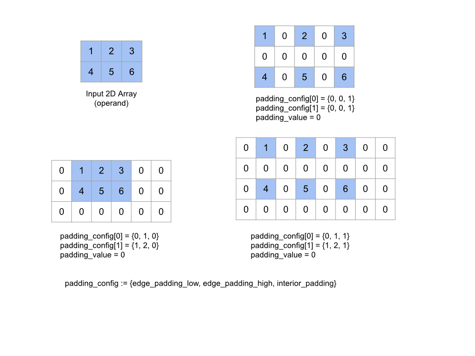
配列の周囲および指定された padding_value で配列の要素間にパディングを追加することで、指定された operand 配列を展開します。padding_config は、各ディメンションの端のパディングと内側のパディングを指定します。
PaddingConfig は PaddingConfigDimension の繰り返しフィールドで、ディメンションごとに 3 つのフィールド(edge_padding_low、edge_padding_high、interior_padding)が含まれています。
edge_padding_low と edge_padding_high は、各ディメンションのローエンド(インデックス 0 の次)とハイエンド(最も高いインデックスの次)に追加するパディングの量をそれぞれ指定します。端のパディングの量は負の数にすることができます。負のパディングの絶対値は、指定したディメンションから削除する要素の数を示します。
interior_padding は、各寸法の任意の 2 つの要素間に追加されるパディングの量を指定します。負の値は指定できません。内部パディングはエッジ パディングの前に論理的に発生するため、負エッジ パディングの場合、要素は内部パディング オペランドから削除されます。
エッジ パディングのペアがすべて(0, 0)で、内部パディングの値がすべて 0 の場合、この演算は何も行われません。次の図は、2 次元配列のさまざまな edge_padding 値と interior_padding 値の例を示しています。
Recv
XlaBuilder::Recv もご覧ください。
Recv(shape, channel_handle)
| 引数 | タイプ | セマンティクス |
|---|---|---|
shape |
Shape |
データの形を変えたり、 |
channel_handle |
ChannelHandle |
送信と受信のペアごとに固有の識別子 |
同じチャネル ハンドルを共有する別の計算の Send 命令から、指定されたシェイプのデータを受け取ります。受信したデータの XLAOp を返します。
Recv オペレーションのクライアント API は同期通信を表します。ただし、この命令は内部的に 2 つの HLO 命令(Recv と RecvDone)に分解され、非同期データ転送が可能になります。HloInstruction::CreateRecv と HloInstruction::CreateRecvDone もご覧ください。
Recv(const Shape& shape, int64 channel_id)
同じ channel_id の Send 命令からデータを受信するために必要なリソースを割り当てます。割り当てられたリソースのコンテキストを返します。これは、次の RecvDone 命令でデータ転送の完了を待機するために使用されます。コンテキストは {受信バッファ(シェイプ)、リクエスト識別子(U32)} のタプルであり、RecvDone 命令でのみ使用できます。
RecvDone(HloInstruction context)
Recv 命令によって作成されたコンテキストが与えられると、データ転送が完了するまで待機し、受信したデータを返します。
Reduce(減らす)
XlaBuilder::Reduce もご覧ください。
1 つ以上の配列にリダクション関数を並列に適用します。
Reduce(operands..., init_values..., computation, dimensions)
| 引数 | タイプ | セマンティクス |
|---|---|---|
operands |
N XlaOp のシーケンス |
T_0, ..., T_{N-1} 型の N 個の配列。 |
init_values |
N XlaOp のシーケンス |
T_0, ..., T_{N-1} 型の N 個のスカラー。 |
computation |
XlaComputation |
T_0, ..., T_{N-1}, T_0, ..., T_{N-1} -> Collate(T_0, ..., T_{N-1}) 型の計算。 |
dimensions |
int64 配列 |
削減するディメンションの順序なし配列。 |
ここで
- N は 1 以上である必要があります。
- 計算は「おおまかに」連想的に行う必要があります(以下を参照)。
- 入力配列はすべて同じディメンションである必要があります。
- すべての初期値は
computationの下で ID を形成する必要があります。 N = 1の場合、Collate(T)はTです。N > 1の場合、Collate(T_0, ..., T_{N-1})はT型のN要素のタプルです。
この演算は、各入力配列の 1 つ以上の次元をスカラーに減らします。返される各配列のランクは rank(operand) - len(dimensions) です。演算の出力は Collate(Q_0, ..., Q_N) です。ここで、Q_i は T_i 型の配列です。そのディメンションは次のとおりです。
異なるバックエンドで削減計算を再度関連付けることができます。加算などの一部のリダクション関数は浮動小数点数に対して結合ではないため、数値に差異が生じる可能性があります。ただし、データの範囲が限られている場合、ほとんどの実用的な用途では、浮動小数点の加算で十分結合的であると言えます。
例
値が [10, 11,
12, 13] で、削減関数 f(これは computation)を使用して、単一の 1 次元配列で 1 つのディメンションにわたって削減する場合、次のように計算できます。
f(10, f(11, f(12, f(init_value, 13)))
他にも多くの方法があります。
f(init_value, f(f(10, f(init_value, 11)), f(f(init_value, 12), f(init_value, 13))))
次に、削減を実装する方法の大まかな擬似コード例を示します。初期値を 0 としてリダクションの計算に総和を使用しています。
result_shape <- remove all dims in dimensions from operand_shape

# Iterate over all elements in result_shape. The number of r's here is equal
# to the rank of the result
for r0 in range(result_shape[0]), r1 in range(result_shape[1]), ...:
  # Initialize this result element
  result[r0, r1...] <- 0

  # Iterate over all the reduction dimensions
  for d0 in range(dimensions[0]), d1 in range(dimensions[1]), ...:
    # Increment the result element with the value of the operand's element.
    # The index of the operand's element is constructed from all ri's and di's
    # in the right order (by construction ri's and di's together index over the
    # whole operand shape).
    result[r0, r1...] += operand[ri... di]
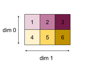
2 次元配列(行列)を縮小する例を次に示します。シェイプはランク 2、ディメンション 0 はサイズ 2、ディメンション 1 はサイズ 3 です。
「add」関数でディメンション 0 または 1 を縮小した結果:
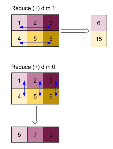
なお、リダクション結果はどちらも 1 次元配列です。この図では、見やすくするため、一方を列、もう一方を行として示しています。
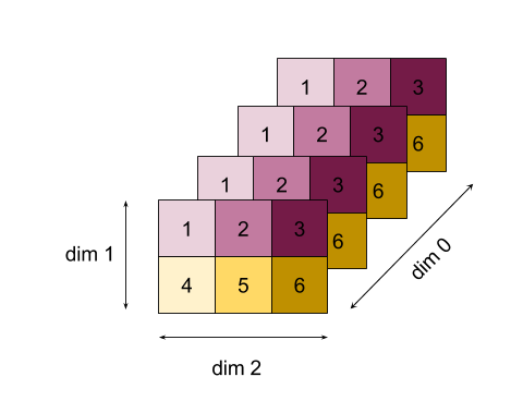
より複雑な例として、3D 配列を示します。ランクは 3、サイズ 4 のディメンション 0、サイズ 2 のディメンション 1、サイズ 3 のディメンション 2 です。わかりやすくするために、値 1 ~ 6 がディメンション 0 に複製されます。
2D の例と同様に、1 つの次元だけを縮小できます。たとえば、ディメンション 0 を減らすと、ディメンション 0 のすべての値がスカラーに折りたたまれたランク 2 の配列になります。
|  4   8  12 |
| 16  20  24 |
ディメンション 2 を減らすと、ディメンション 2 のすべての値がスカラーに折りたたまれたランク 2 配列も得られます。
| 6  15 |
| 6  15 |
| 6  15 |
| 6  15 |
入力に含まれる残りのディメンション間の相対的な順序は出力で保持されますが、一部のディメンションには(ランクが変更されたため)新しい数値が割り当てられることがあります。
また、複数の次元を縮小することもできます。次元 0 と 1 を加算すると、1 次元配列 [20, 28, 36] が生成されます。
3 次元配列をすべての次元にわたって縮小すると、スカラー 84 が生成されます。
Variadic Reduce
N > 1 の場合、すべての入力に同時に適用されるため、Reduce 関数の適用はやや複雑になります。オペランドは、次の順序で計算に提供されます。
- 第 1 オペランドの縮小値を実行する
- ...
- N 番目のオペランドの縮小値を実行する
- 第 1 オペランドの入力値
- ...
- N 番目のオペランドの入力値
たとえば、次のリダクション関数を使用して、1 次元配列の max と argmax を並列に計算できます。
f: (Float, Int, Float, Int) -> Float, Int
f(max, argmax, value, index):
  if value >= max:
    return (value, index)
  else:
    return (max, argmax)
1 次元入力配列 V = Float[N], K = Int[N] と init 値 I_V = Float, I_K = Int の場合、唯一の入力ディメンションで縮小した結果の f_(N-1) は、次の再帰的な適用時と同等です。
f_0 = f(I_V, I_K, V_0, K_0)
f_1 = f(f_0.first, f_0.second, V_1, K_1)
...
f_(N-1) = f(f_(N-2).first, f_(N-2).second, V_(N-1), K_(N-1))
この削減を値の配列と連続したインデックスの配列(iota)に適用すると、配列全体で同じ反復処理が行われ、最大値とマッチング インデックスを含むタプルが返されます。
ReducePrecision
XlaBuilder::ReducePrecision もご覧ください。
浮動小数点値を低精度形式(IEEE-FP16 など)に変換してから元の形式に戻す場合の影響をモデル化します。低精度形式の指数と仮数のビット数は任意に指定できますが、すべてのビットサイズがすべてのハードウェア実装でサポートされているとは限りません。
ReducePrecision(operand, mantissa_bits, exponent_bits)
| 引数 | タイプ | セマンティクス |
|---|---|---|
operand |
XlaOp |
浮動小数点型 T の配列。 |
exponent_bits |
int32 |
低精度形式の指数ビット数 |
mantissa_bits |
int32 |
低精度形式の仮数のビット数 |
結果は T 型の配列になります。入力値は、指定された仮数ビット数で表現できる最も近い値に丸められます(「偶数同数」セマンティクスを使用)。指数ビット数で指定された範囲を超える値はすべて正または負の無限大でクランプされます。NaN 値は保持されますが、正規の NaN 値に変換される場合があります。
低精度形式には、指数ビットが少なくとも 1 つ必要です(ゼロと無限大を区別するため、どちらもゼロの仮数を持つため)。また、指数ビット数が負でない数でなければなりません。指数または仮数のビットの数が、T 型の対応する値を超えることがあります。この場合、変換の対応する部分は何も行いません。
ReduceScatter
XlaBuilder::ReduceScatter もご覧ください。
ReduceScatter は、AllReduce を効果的に行い、その結果を scatter_dimension に沿って shard_count ブロックに分割し、レプリカ グループ内のレプリカ i が ith シャードを受け取る集合オペレーションです。
ReduceScatter(operand, computation, scatter_dim, shard_count,
replica_group_ids, channel_id)
| 引数 | タイプ | セマンティクス |
|---|---|---|
operand |
XlaOp |
レプリカ全体で削減する配列の配列または空でないタプル。 |
computation |
XlaComputation |
削減計算 |
scatter_dimension |
int64 |
散布するディメンション。 |
shard_count |
int64 |
分割するブロック数 scatter_dimension |
replica_groups |
int64 のベクトルのベクトル |
リダクションが行われるグループ |
channel_id |
省略可 int64 |
モジュール間通信用のチャネル ID(省略可) |
operandが配列のタプルの場合、タプルの各要素に対して Reduce-scatter が実行されます。replica_groupsは、削減が行われるレプリカ グループのリストです(現在のレプリカのレプリカ ID は、ReplicaIdを使用して取得できます)。各グループ内のレプリカの順序によって、all-reduce の結果が分散される順序が決まります。replica_groupsは空にするか(この場合、すべてのレプリカが 1 つのグループに属している)、またはレプリカの数と同じ数の要素を含める必要があります。レプリカ グループが複数ある場合は、すべて同じサイズにする必要があります。たとえば、replica_groups = {0, 2}, {1, 3}は、レプリカ0と2、および1と3の間でデータを削減し、結果を分散させます。shard_countは、各レプリカ グループのサイズです。これは、replica_groupsが空の場合に必要になります。replica_groupsが空でない場合、shard_countは各レプリカ グループのサイズと同じである必要があります。channel_idはモジュール間通信に使用されます。相互に通信できるのは、同じchannel_idを持つreduce-scatterオペレーションのみです。
出力シェイプは、scatter_dimension が shard_count 分の 1 に縮小された入力シェイプです。たとえば、2 つのレプリカがあり、2 つのレプリカでオペランドの値が [1.0, 2.25] と [3.0, 5.25] である場合、scatter_dim が 0 であるこの演算からの出力値は、最初のレプリカでは [4.0]、2 番目のレプリカでは [7.5] になります。
ReduceWindow
XlaBuilder::ReduceWindow もご覧ください。
N 個の多次元配列のシーケンスの各ウィンドウ内のすべての要素にリダクション関数を適用し、出力として N 個の多次元配列の単一または N 個のタプルを生成します。各出力配列には、ウィンドウの有効な位置の数と同じ数の要素が含まれます。プーリング レイヤは ReduceWindow で表すことができます。Reduce と同様に、適用される computation には常に左側の init_values が渡されます。
ReduceWindow(operands..., init_values..., computation, window_dimensions,
window_strides, padding)
| 引数 | タイプ | セマンティクス |
|---|---|---|
operands |
N XlaOps |
T_0,..., T_{N-1} 型の N 個の多次元配列のシーケンス。それぞれがウィンドウが配置されるベース領域を表します。 |
init_values |
N XlaOps |
リダクションの N 個の開始値(N 個のオペランドのそれぞれに 1 つずつ)。詳しくは、Reduce をご覧ください。 |
computation |
XlaComputation |
T_0, ..., T_{N-1}, T_0, ..., T_{N-1} -> Collate(T_0, ..., T_{N-1}) 型のリダクション関数。すべての入力オペランドの各ウィンドウ内の要素に適用されます。 |
window_dimensions |
ArraySlice<int64> |
ウィンドウ ディメンション値の整数の配列 |
window_strides |
ArraySlice<int64> |
ウィンドウ ストライド値の整数の配列 |
base_dilations |
ArraySlice<int64> |
基本拡張値の整数の配列 |
window_dilations |
ArraySlice<int64> |
ウィンドウ拡張値の整数の配列 |
padding |
Padding |
ウィンドウのパディング タイプ(ストライドが 1 の場合に入力と同じ出力形状になるようにパディングする Padding::kSame。またはパディングを使用せず、ウィンドウが収まらないと「停止」する Padding::kValid) |
ここで
- N は 1 以上である必要があります。
- 入力配列はすべて同じディメンションである必要があります。
N = 1の場合、Collate(T)はTです。N > 1の場合、Collate(T_0, ..., T_{N-1})は(T0,...T{N-1})型のN要素のタプルです。
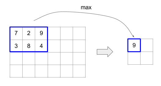
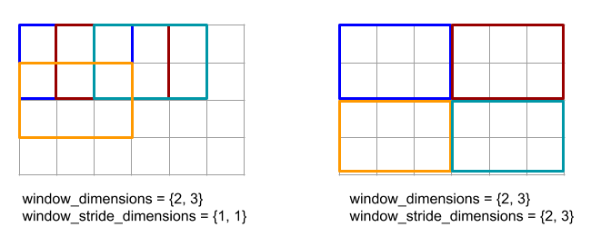
以下のコードと図は、ReduceWindow の使用例を示しています。入力はサイズ [4x6] の行列で、window_dimensions と window_stride_dimensions はどちらも [2x3] です。
// Create a computation for the reduction (maximum).
XlaComputation max;
{
  XlaBuilder builder(client_, "max");
  auto y = builder.Parameter(0, ShapeUtil::MakeShape(F32, {}), "y");
  auto x = builder.Parameter(1, ShapeUtil::MakeShape(F32, {}), "x");
  builder.Max(y, x);
  max = builder.Build().value();
}

// Create a ReduceWindow computation with the max reduction computation.
XlaBuilder builder(client_, "reduce_window_2x3");
auto shape = ShapeUtil::MakeShape(F32, {4, 6});
auto input = builder.Parameter(0, shape, "input");
builder.ReduceWindow(
    input,
    /*init_val=*/builder.ConstantLiteral(LiteralUtil::MinValue(F32)),
    *max,
    /*window_dimensions=*/{2, 3},
    /*window_stride_dimensions=*/{2, 3},
    Padding::kValid);
ディメンションのストライドが 1 の場合、そのディメンション内のウィンドウの位置が、隣接するウィンドウから 1 要素離れていることを指定します。ウィンドウが互いに重複しないようにするには、window_stride_dimensions を window_dimensions と等しくする必要があります。以下の図は、2 つの異なるストライド値の使用を示しています。パディングは入力の各次元に適用され、計算は入力がパディング後の次元で提供された場合と同じです。
重要なパディングの例では、ディメンション 3 を使用してレデューサ ウィンドウの最小値(初期値は MAX_FLOAT)を計算し、入力配列 [10000, 1000, 100, 10, 1] でストライド 2 を計算することを検討してください。パディング kValid により、2 つの有効なウィンドウ([10000, 1000, 100] と [100, 10, 1])の最小値が計算され、出力は [100, 1] になります。まず kSame をパディングすると、両側に初期要素を追加して [MAX_VALUE, 10000, 1000, 100, 10, 1,
MAX_VALUE] を得ることで、Reduce-window の後の形状がストライド 1 の入力と同じになるように配列がパディングされます。パディングされた配列に対して Reduce-window を実行すると、3 つのウィンドウ [MAX_VALUE, 10000, 1000]、[1000, 100, 10]、[10, 1, MAX_VALUE] で動作し、[1000, 10, 1] が生成されます。
リダクション関数の評価順序は任意であり、非決定的であることもあります。したがって、リダクション関数が再関連付けの影響を受けすぎないようにしてください。詳細については、Reduce のコンテキストにおける関連付けに関する説明をご覧ください。
ReplicaId
XlaBuilder::ReplicaId もご覧ください。
レプリカの一意の ID(U32 スカラー)を返します。
ReplicaId()
各レプリカの一意の ID は、[0, N) 区間の符号なし整数です。ここで、N はレプリカの数です。すべてのレプリカが同じプログラムを実行しているため、プログラム内で ReplicaId() を呼び出すと、レプリカごとに異なる値を返します。
Reshape
XlaBuilder::Reshape および Collapse オペレーションもご覧ください。
配列の次元を新しい構成に変更します。
Reshape(operand, new_sizes)
Reshape(operand, dimensions, new_sizes)
| 引数 | タイプ | セマンティクス |
|---|---|---|
operand |
XlaOp |
T 型の配列 |
dimensions |
int64 個のベクター |
ディメンションが折りたたまれる順序 |
new_sizes |
int64 個のベクター |
新しい次元のサイズのベクトル |
概念的には、再形成処理では、まず配列をデータ値の 1 次元ベクトルにフラット化してから、このベクトルを新しいシェイプに改良します。入力引数は、T 型の任意の配列、ディメンション インデックスのコンパイル時定数ベクトル、結果のディメンション サイズのコンパイル時定数ベクトルです。dimension ベクトルの値を指定する場合、その値はすべての T 次元の順列でなければなりません。指定しない場合のデフォルトは {0, ..., rank - 1} です。dimensions のディメンションの順序は、入力配列を 1 つのディメンションに折りたたむループのネスト内で、最も変化の遅いディメンション(最もメジャー)から最も変更の早いディメンション(最もマイナー)の順です。new_sizes ベクトルによって、出力配列のサイズが決まります。new_sizes のインデックス 0 の値はディメンション 0 のサイズで、インデックス 1 の値はディメンション 1 のサイズです。new_size ディメンションの積は、オペランドのディメンション サイズの積と等しくなる必要があります。折りたたまれた配列を new_sizes で定義される多次元配列に絞り込むと、new_sizes のディメンションは、最も変化の少ない(最もメジャー)から最も速い(最もマイナー)の順で並べられます。
たとえば、v を 24 個の要素の配列とします。
let v = f32[4x2x3] { { {10, 11, 12}, {15, 16, 17} },
                    { {20, 21, 22}, {25, 26, 27} },
                    { {30, 31, 32}, {35, 36, 37} },
                    { {40, 41, 42}, {45, 46, 47} } };

In-order collapse:
let v012_24 = Reshape(v, {0,1,2}, {24});
then v012_24 == f32[24] {10, 11, 12, 15, 16, 17, 20, 21, 22, 25, 26, 27,
                         30, 31, 32, 35, 36, 37, 40, 41, 42, 45, 46, 47};

let v012_83 = Reshape(v, {0,1,2}, {8,3});
then v012_83 == f32[8x3] { {10, 11, 12}, {15, 16, 17},
                          {20, 21, 22}, {25, 26, 27},
                          {30, 31, 32}, {35, 36, 37},
                          {40, 41, 42}, {45, 46, 47} };

Out-of-order collapse:
let v021_24 = Reshape(v, {1,2,0}, {24});
then v012_24 == f32[24]  {10, 20, 30, 40, 11, 21, 31, 41, 12, 22, 32, 42,
                          15, 25, 35, 45, 16, 26, 36, 46, 17, 27, 37, 47};

let v021_83 = Reshape(v, {1,2,0}, {8,3});
then v021_83 == f32[8x3] { {10, 20, 30}, {40, 11, 21},
                          {31, 41, 12}, {22, 32, 42},
                          {15, 25, 35}, {45, 16, 26},
                          {36, 46, 17}, {27, 37, 47} };


let v021_262 = Reshape(v, {1,2,0}, {2,6,2});
then v021_262 == f32[2x6x2] { { {10, 20}, {30, 40},
                              {11, 21}, {31, 41},
                              {12, 22}, {32, 42} },
                             { {15, 25}, {35, 45},
                              {16, 26}, {36, 46},
                              {17, 27}, {37, 47} } };
特殊なケースとして、形状変更によって単一要素配列をスカラーに変換したり、その逆に変換したりできます。たとえば
Reshape(f32[1x1] { {5} }, {0,1}, {}) == 5;
Reshape(5, {}, {1,1}) == f32[1x1] { {5} };
Rev(リバース)
XlaBuilder::Rev もご覧ください。
Rev(operand, dimensions)
| 引数 | タイプ | セマンティクス |
|---|---|---|
operand |
XlaOp |
T 型の配列 |
dimensions |
ArraySlice<int64> |
逆方向にするディメンション |
指定された dimensions に沿って、operand 配列内の要素の順序を逆にして、同じ形状の出力配列を生成します。多次元インデックスにあるオペランド配列の各要素は、変換後のインデックスにある出力配列に格納されます。多次元インデックスは、各次元のインデックスを反転して変換されます。つまり、サイズ N の次元が逆次元の 1 つである場合、そのインデックス i は N - 1 - i に変換されます。
Rev 演算の用途の 1 つは、ニューラル ネットワークでの勾配計算中に、2 つのウィンドウ次元に沿って畳み込み重み配列を反転することです。
RngNormal
XlaBuilder::RngNormal もご覧ください。
正規分布に従って生成された乱数を使って、指定した図形の出力を作成します。 \(N(\mu, \sigma)\) パラメータ \(\mu\) と \(\sigma\)、出力シェイプは浮動小数点の要素型でなければなりません。さらに、パラメータはスカラー値にする必要があります。
RngNormal(mu, sigma, shape)
| 引数 | タイプ | セマンティクス |
|---|---|---|
mu |
XlaOp |
生成された数値の平均を指定する T 型のスカラー |
sigma |
XlaOp |
生成された商品の標準偏差を指定する T 型のスカラー |
shape |
Shape |
T 型の出力シェイプ |
RngUniform
XlaBuilder::RngUniform もご覧ください。
区間 \([a,b)\)にわたる一様分布に従って生成された乱数を使用して、指定されたシェイプの出力を作成します。パラメータと出力要素の型は、ブール型、整数型、または浮動小数点型でなければならず、型は一貫している必要があります。現在、CPU バックエンドと GPU バックエンドは、F64、F32、F16、BF16、S64、U64、S32、U32 のみをサポートしています。また、パラメータはスカラー値である必要があります。 \(b <= a\) 結果が実装で定義されている場合。
RngUniform(a, b, shape)
| 引数 | タイプ | セマンティクス |
|---|---|---|
a |
XlaOp |
間隔の下限を指定する T 型のスカラー |
b |
XlaOp |
間隔の上限を指定する T 型のスカラー |
shape |
Shape |
T 型の出力シェイプ |
RngBitGenerator
指定されたアルゴリズム(またはバックエンドのデフォルト)を使用して、均一なランダムビットが入力された特定のシェイプの出力を生成し、更新された状態(初期状態と同じシェイプ)と生成されたランダムデータを返します。
初期状態は、現在の乱数生成の初期状態です。必要な形状と有効な値は、使用するアルゴリズムによって異なります。
出力は、初期状態の決定論的関数であることが保証されますが、バックエンドと異なるコンパイラ バージョンとの間で確定的であるという保証はありません。
RngBitGenerator(algorithm, key, shape)
| 引数 | タイプ | セマンティクス |
|---|---|---|
algorithm |
RandomAlgorithm |
使用する PRNG アルゴリズム。 |
initial_state |
XlaOp |
PRNG アルゴリズムの初期状態。 |
shape |
Shape |
生成されたデータの出力シェイプ。 |
algorithm に使用可能な値:
rng_default: バックエンド固有のシェイプ要件があるバックエンド固有のアルゴリズム。rng_three_fry: ThreeFry カウンタベースの PRNG アルゴリズム。initial_stateのシェイプは任意の値を持つu64[2]です。Salmon et al. SC 2011. 並列乱数: 1、2、3 と同じくらい簡単です。rng_philox: 乱数を並列に生成する Philox アルゴリズム。initial_stateのシェイプは任意の値を持つu64[3]です。Salmon et al. SC 2011. 並列乱数: 1、2、3 と同じくらい簡単です。
散布
XLA 散布演算は、入力配列 operands の値である一連の結果を生成します。update_computation を使用して、updates の値のシーケンスで更新される複数のスライス(scatter_indices で指定されたインデックス)があります。
XlaBuilder::Scatter もご覧ください。
scatter(operands..., scatter_indices, updates..., update_computation,
index_vector_dim, update_window_dims, inserted_window_dims,
scatter_dims_to_operand_dims)
| 引数 | タイプ | セマンティクス |
|---|---|---|
operands |
N XlaOp のシーケンス |
分散させる T_0, ..., T_N 型の N 個の配列。 |
scatter_indices |
XlaOp |
分散させるスライスの開始インデックスを含む配列。 |
updates |
N XlaOp のシーケンス |
T_0, ..., T_N 型の N 個の配列。updates[i] には、operands[i] の分散に使用する必要がある値が含まれています。 |
update_computation |
XlaComputation |
入力配列内の既存の値と分散中の更新を結合するために使用される計算。この計算は T_0, ..., T_N, T_0, ..., T_N -> Collate(T_0, ..., T_N) 型にする必要があります。 |
index_vector_dim |
int64 |
開始インデックスを含む scatter_indices のディメンション。 |
update_window_dims |
ArraySlice<int64> |
ウィンドウ ディメンションである updates シェイプのディメンションのセット。 |
inserted_window_dims |
ArraySlice<int64> |
updates シェイプに挿入する必要があるウィンドウ ディメンションのセット。 |
scatter_dims_to_operand_dims |
ArraySlice<int64> |
散布型インデックスからオペランド インデックス空間へのディメンション マップ。この配列は、i から scatter_dims_to_operand_dims[i] へのマッピングとして解釈されます。1 対 1 で、合計にする必要があります。 |
indices_are_sorted |
bool |
インデックスが呼び出し元によって確実に並べ替えられるかどうか。 |
ここで
- N は 1 以上である必要があります。
operands[0]、...、operands[N-1] はすべて同じディメンションである必要があります。updates[0]、...、updates[N-1] はすべて同じディメンションである必要があります。N = 1の場合、Collate(T)はTです。N > 1の場合、Collate(T_0, ..., T_N)はT型のN要素のタプルです。
index_vector_dim が scatter_indices.rank と等しい場合、scatter_indices の末尾の 1 ディメンションが暗黙的に考慮されます。
ArraySlice<int64> タイプの update_scatter_dims を、update_window_dims にない updates シェイプのディメンションのセットを昇順で定義します。
scatter の引数は次の制約に従う必要があります。
各
updates配列はランクupdate_window_dims.size + scatter_indices.rank - 1である必要があります。各
updates配列のディメンションiの境界は、次に準拠している必要があります。iがupdate_window_dimsに存在する場合(つまり、一部のkでupdate_window_dims[k] と等しい場合)、updatesのディメンションiの境界は、inserted_window_dimsを考慮した後、operandの対応する境界を超えてはなりません(adjusted_window_bounds[k]。adjusted_window_bounds[k] には、インデックスinserted_window_dimsの境界が削除されたoperandの境界が含まれます)。iがupdate_scatter_dimsに存在する場合(つまり、一部のkでupdate_scatter_dims[k] と等しい場合)、updatesのディメンションiの境界は、index_vector_dimをスキップして、対応するscatter_indicesの境界と等しくなければなりません(k<index_vector_dimの場合はscatter_indices.shape.dims[k]、そうでない場合はscatter_indices.shape.dims[k+1])。
update_window_dimsは昇順で、ディメンション番号の繰り返しはなく、[0, updates.rank)の範囲内である必要があります。inserted_window_dimsは昇順で、ディメンション番号の繰り返しはなく、[0, operand.rank)の範囲内である必要があります。operand.rankは、update_window_dims.sizeとinserted_window_dims.sizeの合計と等しくなる必要があります。scatter_dims_to_operand_dims.sizeはscatter_indices.shape.dims[index_vector_dim] と等しくなければならず、その値は[0, operand.rank)の範囲内にある必要があります。
各 updates 配列の特定のインデックス U について、このアップデートを適用する必要がある、対応する operands 配列内の対応するインデックス I は次のように計算されます。
G= {U[k] forupdate_scatter_dimsinupdate_scatter_dims}。Gを使用して、S[i] =scatter_indices[ combine(G,i)] のようにscatter_indices配列のインデックス ベクトルSをルックアップします。ここで、Combine(A, b) は位置index_vector_dimの b を A に挿入します。kscatter_dims_to_operand_dimsのマップを使用してSを分散し、Sを使用してoperandにインデックスSinを作成します。より正式に次のように記述します。Sin[scatter_dims_to_operand_dims[k]] =S[k](k<scatter_dims_to_operand_dims.sizeの場合)。Sin[_] =0。
inserted_window_dimsに従い、Uのupdate_window_dimsにインデックスを分散させて、各operands配列にインデックスWinを作成します。より正式に次のように記述します。Win[window_dims_to_operand_dims(k)] =U[k]kがupdate_window_dimsの場合、window_dims_to_operand_dimsはドメイン [0,update_window_dims.size] と範囲 [0,operand.rank) \inserted_window_dimsを持つ単調関数です。(たとえば、update_window_dims.sizeが4、operand.rankが6、inserted_window_dimsが {0、2} の場合、window_dims_to_operand_dimsは {0→1、1→3、2→4、3→5} です)。Win[_] =0。
IはWin+Sinです。「+」は要素単位の加算です。
要約すると、scatter 操作は次のように定義できます。
outputをoperandsで初期化します。つまり、operands[J] 配列内のすべてのインデックスOについて、すべてのインデックスJに対して初期化します。
output[J][O] =operands[J][O]updates[J] 配列のすべてのインデックスUと、operand[J] 配列の対応するインデックスO(Oがoutputの有効なインデックスの場合):
(output[0][O], ...,output[N-1][O]) =update_computation(output[0][O], ..., ,output[N-1][O],updates[0][U], ...,updates[N-1][U])
更新が適用される順序は非決定的です。そのため、updates 内の複数のインデックスが operands 内の同じインデックスを参照している場合、output 内の対応する値は非決定的になります。
update_computation に渡される最初のパラメータは常に output 配列の現在の値であり、2 番目のパラメータは常に updates 配列の値であることに注意してください。これは、特に update_computation が可換でない場合に重要です。
indices_are_sorted が true に設定されている場合、XLA は start_indices がユーザーによって(start_index_map の昇順で)並べ替えられていると想定できます。含まれていない場合、セマンティクスは実装が定義されています。
非公式には、scatter 演算は collect 演算の逆とみなすことができます。すなわち、scatter 演算は、対応する collect 演算によって抽出された入力内の要素を更新します。
詳細な非公式の説明と例については、Gather の「非公式な説明」セクションをご覧ください。
選択
XlaBuilder::Select もご覧ください。
述語配列の値に基づいて、2 つの入力配列の要素から出力配列を作成します。
Select(pred, on_true, on_false)
| 引数 | タイプ | セマンティクス |
|---|---|---|
pred |
XlaOp |
PRED 型の配列 |
on_true |
XlaOp |
T 型の配列 |
on_false |
XlaOp |
T 型の配列 |
配列 on_true と on_false の形状は同じである必要があります。これは出力配列の形状でもあります。配列 pred は on_true および on_false と同じ次元で、要素タイプは PRED である必要があります。
pred の各要素 P について、P の値が true の場合は on_true から、P の値が false の場合は on_false から、出力配列の対応する要素が取得されます。ブロードキャストの制限付き形式として、pred は PRED 型のスカラーにできます。この場合、出力配列は、pred が true の場合は on_true から、pred が false の場合は on_false からすべて取得されます。
非スカラー pred の例:
let pred: PRED[4] = {true, false, false, true};
let v1: s32[4] = {1, 2, 3, 4};
let v2: s32[4] = {100, 200, 300, 400};
==>
Select(pred, v1, v2) = s32[4]{1, 200, 300, 4};
スカラー pred を使用した例:
let pred: PRED = true;
let v1: s32[4] = {1, 2, 3, 4};
let v2: s32[4] = {100, 200, 300, 400};
==>
Select(pred, v1, v2) = s32[4]{1, 2, 3, 4};
タプル間の選択がサポートされています。タプルは、この目的のためにスカラー型とみなされます。on_true と on_false がタプル(同じ形状にする必要がある)の場合、pred は PRED 型のスカラーである必要があります。
SelectAndScatter
XlaBuilder::SelectAndScatter もご覧ください。
この演算は、最初に operand 配列の ReduceWindow を計算して各ウィンドウから要素を選択し、次に source 配列を選択された要素のインデックスに分散してオペランド配列と同じ形状の出力配列を作成する複合演算と考えることができます。バイナリ select 関数は、各ウィンドウ全体に適用して各ウィンドウから要素を選択するために使用されます。この関数は、最初のパラメータのインデックス ベクトルが 2 番目のパラメータのインデックス ベクトルよりも辞書順で小さいというプロパティで呼び出されます。select 関数は、最初のパラメータが選択された場合は true を返し、2 番目のパラメータが選択された場合は false を返します。関数は推移性を保持する必要があります(つまり、select(a, b) と select(b, c) が true の場合、select(a, c) も true である)。これにより、選択された要素が特定のウィンドウで走査される要素の順序に依存しなくなります。
関数 scatter は、出力配列で選択されたインデックスごとに適用されます。このメソッドは次の 2 つのスカラー パラメータを取ります。
- 出力配列で、選択されたインデックスの現在の値
- 選択したインデックスに適用される
sourceからの散布値
2 つのパラメータを結合して、出力配列で選択されたインデックスの値を更新するために使用されるスカラー値を返します。初期設定では、出力配列のすべてのインデックスが init_value に設定されます。
出力配列は operand 配列と同じ形状になります。source 配列は、operand 配列に ReduceWindow 演算を適用した結果と同じ形状でなければなりません。SelectAndScatter を使用すると、ニューラル ネットワークのプーリング層の勾配値を逆伝播できます。
SelectAndScatter(operand, select, window_dimensions, window_strides,
padding, source, init_value, scatter)
| 引数 | タイプ | セマンティクス |
|---|---|---|
operand |
XlaOp |
ウィンドウがスライドする T 型の配列 |
select |
XlaComputation |
各ウィンドウのすべての要素に適用する T, T -> PRED 型のバイナリ計算。最初のパラメータが選択された場合は true を返し、2 番目のパラメータが選択された場合は false を返します |
window_dimensions |
ArraySlice<int64> |
ウィンドウ ディメンション値の整数の配列 |
window_strides |
ArraySlice<int64> |
ウィンドウ ストライド値の整数の配列 |
padding |
Padding |
ウィンドウのパディング タイプ(Padding::kSame または Padding::kValid) |
source |
XlaOp |
散布する値を持つ T 型の配列 |
init_value |
XlaOp |
出力配列の初期値に対する T 型のスカラー値 |
scatter |
XlaComputation |
T, T -> T 型のバイナリ計算。散布ソースの各要素をそのデスティネーション要素とともに適用します。 |
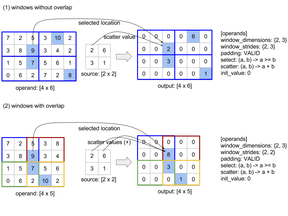
以下の図は、SelectAndScatter の使用例を示しています。select 関数でパラメータの最大値を計算しています。なお、下の図(2)のようにウィンドウが重なっている場合、operand 配列のインデックスは、異なるウィンドウで複数回選択される可能性があります。この図では、値 9 の要素が上位のウィンドウ(青と赤)の両方で選択され、バイナリ加算 scatter 関数は値 8(2 + 6)の出力要素を生成します。
scatter 関数の評価順序は任意であり、非決定的な場合もあります。したがって、scatter 関数が再関連付けの影響を過度に受けないようにする必要があります。詳細については、Reduce のコンテキストにおける関連付けに関する説明をご覧ください。
送信
XlaBuilder::Send もご覧ください。
Send(operand, channel_handle)
| 引数 | タイプ | セマンティクス |
|---|---|---|
operand |
XlaOp |
送信するデータ(T 型の配列) |
channel_handle |
ChannelHandle |
送信と受信のペアごとに固有の識別子 |
同じチャネル ハンドルを共有する別の計算の Recv 命令に、指定されたオペランド データを送信します。データを返しません。
Recv オペレーションと同様に、Send オペレーションのクライアント API は同期通信を表し、非同期データ転送を可能にするために 2 つの HLO 命令(Send と SendDone)に内部的に分解されます。HloInstruction::CreateSend と HloInstruction::CreateSendDone もご覧ください。
Send(HloInstruction operand, int64 channel_id)
同じチャネル ID の Recv 命令によって割り当てられたリソースへの、オペランドの非同期転送を開始します。コンテキストを返します。コンテキストは、次の SendDone 命令によって使用され、データ転送の完了を待機します。コンテキストは {オペランド(シェイプ)、リクエスト識別子(U32)} のタプルであり、SendDone 命令でのみ使用できます。
SendDone(HloInstruction context)
Send 命令によって作成されたコンテキストを与えられ、データ転送が完了するまで待ちます。この命令はデータを返しません。
チャンネル設定の手順
各チャネル(Recv、RecvDone、Send、SendDone)の 4 つの命令の実行順序は次のとおりです。
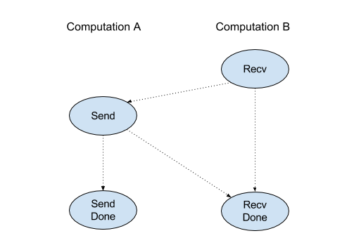
Sendより前にRecvが発生RecvDoneより前にSendが発生RecvDoneより前にRecvが発生SendDoneより前にSendが発生
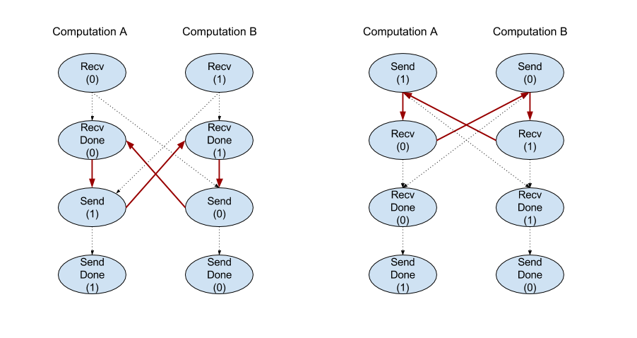
バックエンド コンパイラが、チャネル命令を介して通信する計算ごとに線形スケジュールを生成する場合、計算間でサイクルがあってはなりません。たとえば、以下のスケジュールはデッドロックにつながります。
スライス
XlaBuilder::Slice もご覧ください。
スライスにより、入力配列からサブ配列が抽出されます。サブ配列は入力と同じランクであり、入力配列内の境界ボックス内の値を含みます。ここで、境界ボックスのディメンションとインデックスは、スライス演算への引数として渡されます。
Slice(operand, start_indices, limit_indices, strides)
| 引数 | タイプ | セマンティクス |
|---|---|---|
operand |
XlaOp |
T 型の N 次元配列 |
start_indices |
ArraySlice<int64> |
各ディメンションのスライスの開始インデックスを含む N 個の整数のリスト。0 以上の値を指定してください。 |
limit_indices |
ArraySlice<int64> |
各ディメンションのスライスの終了インデックス(排他的)を含む N 個の整数のリスト。各値は、ディメンションのそれぞれの start_indices 値以上かつディメンションのサイズ以下にする必要があります。 |
strides |
ArraySlice<int64> |
スライスの入力ストライドを決定する N 個の整数のリスト。スライスは、ディメンション d のすべての strides[d] 要素を選択します。 |
1 次元の例:
let a = {0.0, 1.0, 2.0, 3.0, 4.0}
Slice(a, {2}, {4}) produces:
  {2.0, 3.0}
2 次元の例:
let b =
 { {0.0,  1.0,  2.0},
   {3.0,  4.0,  5.0},
   {6.0,  7.0,  8.0},
   {9.0, 10.0, 11.0} }

Slice(b, {2, 1}, {4, 3}) produces:
  { { 7.0,  8.0},
    {10.0, 11.0} }
並べ替え
XlaBuilder::Sort もご覧ください。
Sort(operands, comparator, dimension, is_stable)
| 引数 | タイプ | セマンティクス |
|---|---|---|
operands |
ArraySlice<XlaOp> |
並べ替えるオペランド。 |
comparator |
XlaComputation |
使用するコンパレータの計算。 |
dimension |
int64 |
並べ替えの基準とするディメンション。 |
is_stable |
bool |
安定した並べ替えを使用するかどうか。 |
オペランドを 1 つだけ指定した場合:
オペランドがランク 1 テンソル(配列)の場合、結果は並べ替えられた配列になります。配列を昇順で並べ替えるには、コンパレータで小なりの比較を行う必要があります。正式には、配列が並べ替えられた後、
i < jを持つi, jのすべてのインデックス位置(comparator(value[i], value[j]) = comparator(value[j], value[i]) = falseまたはcomparator(value[i], value[j]) = true)で保持されます。オペランドのランクが高い場合、オペランドは指定されたディメンションに沿って並べ替えられます。たとえば、ランク 2 テンソル(行列)の場合、ディメンション値
0はすべての列を個別に並べ替え、ディメンション値1は各行を個別に並べ替えます。ディメンション番号を指定しない場合、デフォルトで最後のディメンションが選択されます。並べ替えられるディメンションには、ランク 1 の場合と同じ並べ替え順序が適用されます。
n > 1 オペランドを指定した場合:
すべての
nオペランドは、同じ次元のテンソルでなければなりません。テンソルの要素型が異なる場合があります。すべてのオペランドは、個別にではなく、まとめて並べ替えられます。概念的には、オペランドはタプルとして扱われます。インデックス位置
iとjにある各オペランドの要素を入れ替える必要があるかどうかをチェックする場合は、2 * nスカラー パラメータでコンパレータが呼び出されます。ここで、パラメータ2 * kはk-thオペランドのi位置の値に対応し、パラメータ2 * k + 1はk-thオペランドの位置jの値に対応します。したがって、通常、コンパレータはパラメータ2 * kと2 * k + 1を相互に比較し、他のパラメータペアをタイブレーカーとして使用する可能性があります。結果は、(上記のように指定されたディメンションに沿って)並べ替えられたオペランドで構成されるタプルになります。タプルの
i-thオペランドは、Sort のi-thオペランドに対応します。
たとえば、operand0 = [3, 1]、operand1 = [42, 50]、operand2 = [-3.0, 1.1] の 3 つのオペランドがあり、コンパレータが operand0 の値のみを小なり値と比較する場合、その並べ替えの出力はタプル ([1, 3], [50, 42], [1.1, -3.0]) になります。
is_stable が true に設定されている場合、並べ替えが安定することが保証されます。つまり、コンパレータによって等しいとみなされる要素がある場合、等しい値の相対的な順序が保持されます。e1 と e2 の 2 つの要素は、comparator(e1, e2) = comparator(e2, e1) = false の場合にのみ等しくなります。デフォルトでは、is_stable は false に設定されています。
行 / 列の入れ替え
tf.reshape オペレーションもご覧ください。
Transpose(operand)
| 引数 | タイプ | セマンティクス |
|---|---|---|
operand |
XlaOp |
転置するオペランド。 |
permutation |
ArraySlice<int64> |
ディメンションを並べ替える方法。 |
指定された順列でオペランド次元を並べ替えます。つまり ∀ i . 0 ≤ i < rank ⇒ input_dimensions[permutation[i]] = output_dimensions[i] です。
これは Reshape(operand, permut, Permute(permut, operand.shape.dimensions)) と同じです。
TriangularSolve
XlaBuilder::TriangularSolve もご覧ください。
前方代入または後代入法によって、下または上三角係数行列を持つ一次方程式系を解く。リーディング ディメンションに沿ってブロードキャストし、このルーティンは、a と b が与えられた変数 x に対して、行列系 op(a) * x =
b または x * op(a) = b のいずれかを解きます。ここで、op(a) は op(a) = a、op(a) = Transpose(a)、または op(a) = Conj(Transpose(a)) のいずれかです。
TriangularSolve(a, b, left_side, lower, unit_diagonal, transpose_a)
| 引数 | タイプ | セマンティクス |
|---|---|---|
a |
XlaOp |
形状 [..., M, M] を持つ複素数または浮動小数点型のランク > 2 の配列。 |
b |
XlaOp |
left_side が true の場合、[..., M, K] の形をした同じ型のランク > 2 の配列。それ以外の場合は [..., K, M] です。 |
left_side |
bool |
op(a) * x = b(true)または x * op(a) = b(false)の形式の系を解くかどうかを示します。 |
lower |
bool |
a の上向き三角形と下三角形のどちらを使用するかを指定します。 |
unit_diagonal |
bool |
true の場合、a の対角要素が 1 であると想定され、アクセスされません。 |
transpose_a |
Transpose |
a をそのまま使用するか、転置するか、その共役転置を取るかを指定します。 |
入力データは、lower の値に応じて、a の下/上向きの三角形からのみ読み取られます。もう一方の三角形の値は無視されます。出力データは同じ三角形に返されます。他方の三角形の値は実装によって定義されるため、何でもかまいません。
a と b のランクが 2 より大きい場合、これらは行列のバッチとして扱われ、マイナー 2 次元を除くすべてがバッチ ディメンションです。a と b は、同じバッチ ディメンションである必要があります。
タプル型
XlaBuilder::Tuple もご覧ください。
可変数のデータハンドルを含むタプル。各ハンドルは独自の形状を持ちます。
これは C++ の std::tuple に似ています。概念的には次のとおりです。
let v: f32[10] = f32[10]{0, 1, 2, 3, 4, 5, 6, 7, 8, 9};
let s: s32 = 5;
let t: (f32[10], s32) = tuple(v, s);
タプルは、GetTupleElement オペレーションで分解(アクセス)できます。
一方
XlaBuilder::While もご覧ください。
While(condition, body, init)
| 引数 | タイプ | セマンティクス |
|---|---|---|
condition |
XlaComputation |
ループの終了条件を定義する T -> PRED 型の XlaComputation。 |
body |
XlaComputation |
ループの本体を定義する T -> T 型の XlaComputation。 |
init |
T |
condition と body のパラメータの初期値。 |
condition が失敗するまで、body を順次実行します。これは、以下に記載する違いと制限を除き、多くの言語における一般的な while ループと似ています。
WhileノードはT型の値を返します。これは、bodyを最後に実行した結果です。T型の形状は静的に決定され、すべての反復処理で同じにする必要があります。
計算の T パラメータは、最初の反復処理で init 値で初期化され、後続の各反復処理で body の新しい結果に自動的に更新されます。
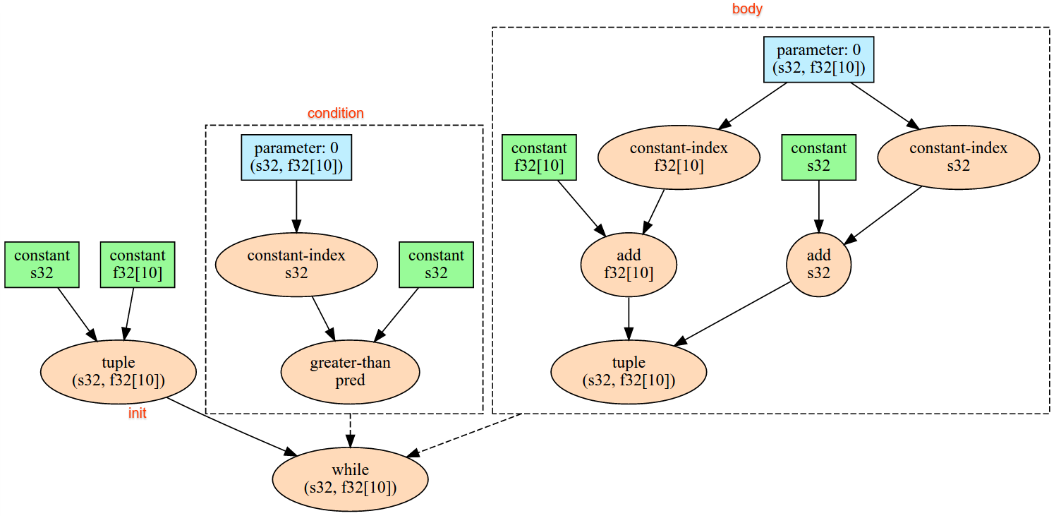
While ノードの主なユースケースの 1 つは、ニューラル ネットワークで繰り返し行われるトレーニングを実装することです。以下に、簡略化した擬似コードをグラフとともに示します。コードは while_test.cc にあります。この例の T 型は Tuple で、反復回数の int32 とアキュムレータの vector[10] で構成されています。1, 000 回の反復処理で、ループは定数ベクトルをアキュムレータに追加し続けています。
// Pseudocode for the computation.
init = {0, zero_vector[10]} // Tuple of int32 and float[10].
result = init;
while (result(0) < 1000) {
  iteration = result(0) + 1;
  new_vector = result(1) + constant_vector[10];
  result = {iteration, new_vector};
}