Veja a seguir a descrição da semântica das operações definidas na interface XlaBuilder. Normalmente, essas operações são mapeadas individualmente para as operações definidas na
interface de RPC em
xla_data.proto.
Uma observação sobre a nomenclatura: o tipo de dados generalizado que o XLA lida é uma matriz de N-dimensional que contém elementos de algum tipo uniforme (como um flutuante de 32 bits). Ao longo de toda a documentação, array é usada para indicar uma matriz de dimensão arbitrária. Por conveniência, os casos especiais têm nomes mais específicos e conhecidos. Por exemplo, um vetor é uma matriz unidimensional e uma matriz é uma matriz bidimensional.
AfterAll
Consulte também
XlaBuilder::AfterAll.
AfterAll usa um número variável de tokens e produz um único token. Os tokens são tipos primitivos que podem ser encadeados entre operações com efeito colateral para impor a ordem. AfterAll pode ser usado como uma mesclagem de tokens para ordenar uma
operação após um conjunto de operações.
AfterAll(operands)
| Argumentos | Tipo | Semântica |
|---|---|---|
operands |
XlaOp |
número variável de tokens |
AllGather
Consulte também
XlaBuilder::AllGather.
Executa a concatenação entre as réplicas.
AllGather(operand, all_gather_dim, shard_count, replica_group_ids,
channel_id)
| Argumentos | Tipo | Semântica |
|---|---|---|
operand
|
XlaOp
|
Matriz para concatenar as réplicas |
all_gather_dim |
int64 |
Dimensão de concatenação |
replica_groups
|
vetor de vetores de
int64 |
Grupos entre os quais a concatenação é realizada |
channel_id
|
int64 opcional
|
ID do canal opcional para comunicação entre módulos |
replica_groupsé uma lista de grupos de réplicas entre os quais a concatenação é realizada (o ID da réplica atual pode ser recuperado usandoReplicaId). A ordem das réplicas em cada grupo determina a ordem em que as entradas estão localizadas no resultado.replica_groupsprecisa estar vazio (nesse caso, todas as réplicas pertencem a um único grupo, ordenadas de0aN - 1) ou conter o mesmo número de elementos que o número de réplicas. Por exemplo,replica_groups = {0, 2}, {1, 3}executa a concatenação entre as réplicas0e2, e1e3.shard_counté o tamanho de cada grupo de réplicas. Precisamos disso nos casos em quereplica_groupsestá vazio.channel_idé usado para comunicação entre módulos: apenas operaçõesall-gathercom o mesmochannel_idpodem se comunicar entre si.
A forma de saída é a forma de entrada com o all_gather_dim tornado shard_count
vezes maior. Por exemplo, se houver duas réplicas e o operando tiver o
valor [1.0, 2.5] e [3.0, 5.25], respectivamente, nas duas réplicas, o
valor de saída dessa operação em que all_gather_dim é 0 será [1.0, 2.5, 3.0,
5.25] em ambas as réplicas.
AllReduce
Consulte também
XlaBuilder::AllReduce.
Executa uma computação personalizada entre as réplicas.
AllReduce(operand, computation, replica_group_ids, channel_id)
| Argumentos | Tipo | Semântica |
|---|---|---|
operand
|
XlaOp
|
Matriz ou uma tupla não vazia de matrizes a serem reduzidas entre as réplicas |
computation |
XlaComputation |
Computação de redução |
replica_groups
|
vetor de vetores de
int64 |
Grupos entre os quais as reduções são realizadas |
channel_id
|
int64 opcional
|
ID do canal opcional para comunicação entre módulos |
- Quando
operandé uma tupla de matrizes, a redução completa é realizada em cada elemento da tupla. replica_groupsé uma lista de grupos de réplicas entre os quais a redução é realizada (o ID da réplica atual pode ser recuperado usandoReplicaId).replica_groupsprecisa estar vazio (nesse caso, todas as réplicas pertencem a um único grupo) ou conter o mesmo número de elementos que o número de réplicas. Por exemplo,replica_groups = {0, 2}, {1, 3}realiza uma redução entre as réplicas0e2, e1e3.channel_idé usado para comunicação entre módulos: apenas operaçõesall-reducecom o mesmochannel_idpodem se comunicar entre si.
A forma de saída é igual à forma de entrada. Por exemplo, se houver duas
réplicas e o operando tiver o valor [1.0, 2.5] e [3.0, 5.25],
respectivamente, nas duas réplicas, o valor de saída desse cálculo de operação e
soma será [4.0, 7.75] nas duas réplicas. Se a entrada for uma tupla, a saída também será.
A computação do resultado de AllReduce requer uma entrada de cada réplica.
Se uma réplica executar um nó AllReduce mais vezes que outra, a
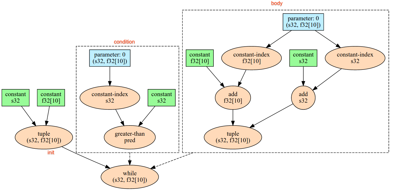
réplica anterior aguardará para sempre. Como as réplicas estão executando o mesmo
programa, não há muitas maneiras de isso acontecer, mas é possível quando
a condição de um loop "while" depende dos dados da entrada e dos dados inseridos
fazem com que a repetição "while" itere mais vezes em uma réplica do que outra.
AllToAll
Consulte também
XlaBuilder::AllToAll.
AllToAll é uma operação coletiva que envia dados de todos os núcleos para todos os núcleos. Ele tem duas fases:
- Fase de dispersão. Em cada núcleo, o operando é dividido em um número de
split_countde blocos ao longo dasplit_dimensions, e os blocos são dispersos para todos os núcleos. Por exemplo, o i-ésimo bloco é enviado para o i-ésimo núcleo. - Fase de coleta. Cada núcleo concatena os blocos recebidos na
concat_dimension.
Os núcleos participantes podem ser configurados da seguinte maneira:
replica_groups: cada ReplicaGroup contém uma lista de IDs de réplica que participam do cálculo (o ID da réplica atual pode ser recuperado usandoReplicaId). AllToAll será aplicado em subgrupos na ordem especificada. Por exemplo,replica_groups = { {1,2,3}, {4,5,0} }significa que um AllToAll será aplicado nas réplicas{1, 2, 3}e, na fase de coleta, os blocos recebidos serão concatenados na mesma ordem de 1, 2, 3. Em seguida, outro AllToAll será aplicado nas réplicas 4, 5, 0, e a ordem de concatenação também será 4, 5, 0. Sereplica_groupsestiver vazio, todas as réplicas pertencerão a um grupo, na ordem de concatenação da aparência delas.
Pré-requisitos:
- O tamanho da dimensão do operando no
split_dimensioné divisível porsplit_count. - O formato do operando não é tupla.
AllToAll(operand, split_dimension, concat_dimension, split_count,
replica_groups)
| Argumentos | Tipo | Semântica |
|---|---|---|
operand |
XlaOp |
matriz de entrada dimensional n |
split_dimension
|
int64
|
Um valor no intervalo [0,
n) que nomeia a dimensão
ao lado do qual o operando é
dividido. |
concat_dimension
|
int64
|
Um valor no intervalo [0,
n) que nomeia a dimensão
ao qual os blocos de divisão
são concatenados. |
split_count
|
int64
|
O número de núcleos que participam dessa operação. Se
replica_groups estiver vazio, será o número de réplicas.
Caso contrário, ele
precisará ser igual ao número
de réplicas em cada grupo. |
replica_groups
|
ReplicaGroup vetor
|
Cada grupo contém uma lista de IDs de réplica. |
Confira abaixo um exemplo de Alltoall.
XlaBuilder b("alltoall");
auto x = Parameter(&b, 0, ShapeUtil::MakeShape(F32, {4, 16}), "x");
AllToAll(x, /*split_dimension=*/1, /*concat_dimension=*/0, /*split_count=*/4);
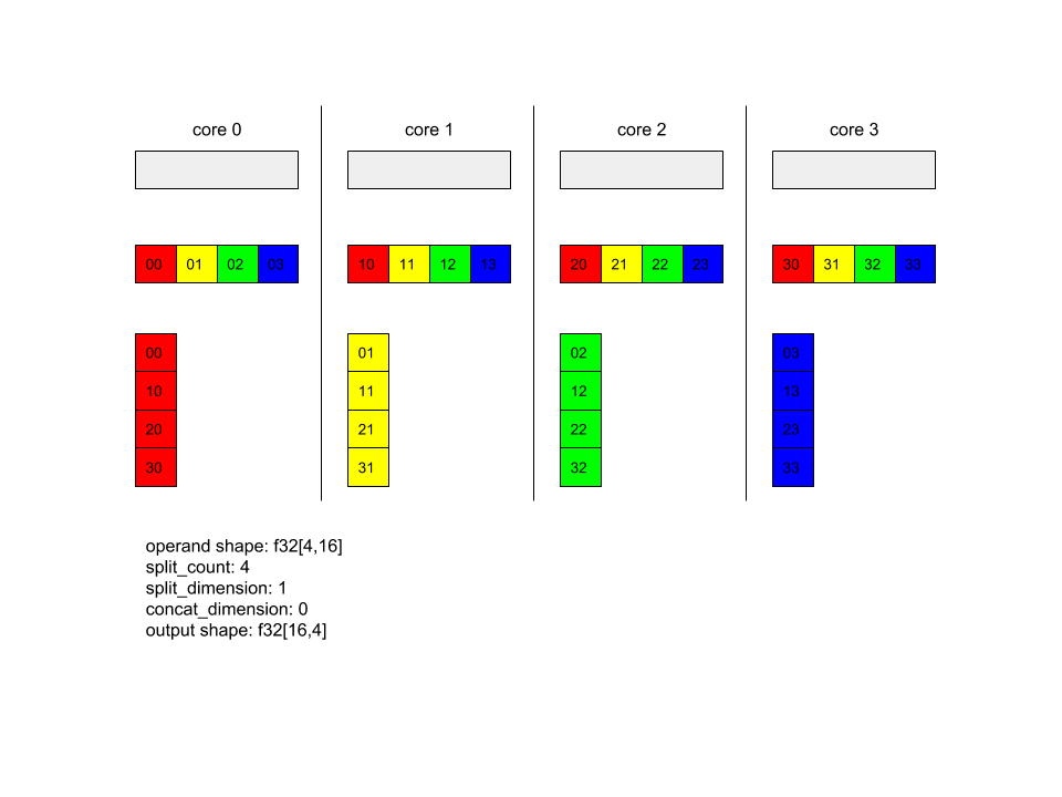
Neste exemplo, há quatro núcleos participando do Alltoall. Em cada núcleo, o operando é dividido em quatro partes ao longo da dimensão 0, de modo que cada parte tenha a forma f32[4,4]. As quatro partes estão espalhadas por todos os núcleos. Em seguida, cada núcleo concatena as partes recebidas na dimensão 1, na ordem do núcleo 0 a 4. Assim, a saída em cada núcleo tem a forma f32[16,4].
BatchNormGrad
Consulte também
XlaBuilder::BatchNormGrad
e o documento original de normalização em lote
para uma descrição detalhada do algoritmo.
Calcula os gradientes da norma de lote.
BatchNormGrad(operand, scale, mean, variance, grad_output, epsilon, feature_index)
| Argumentos | Tipo | Semântica |
|---|---|---|
operand |
XlaOp |
matriz dimensional n a ser normalizada (x) |
scale |
XlaOp |
Matriz unidimensional (\(\gamma\)) |
mean |
XlaOp |
Matriz unidimensional (\(\mu\)) |
variance |
XlaOp |
Matriz unidimensional (\(\sigma^2\)) |
grad_output |
XlaOp |
Gradientes transmitidos para BatchNormTraining (\(\nabla y\)) |
epsilon |
float |
Valor do épsilon (\(\epsilon\)) |
feature_index |
int64 |
Indexar à dimensão do atributo em operand |
Para cada atributo na dimensão (feature_index é o índice da
dimensão em operand), a operação calcula os gradientes em
respeito a operand, offset e scale em todas as outras dimensões. O feature_index precisa ser um índice válido para a dimensão do recurso em operand.
Os três gradientes são definidos pelas seguintes fórmulas, supondo uma matriz 4dimensional como operand e com índice de dimensão de recurso l, tamanho de lote m e tamanhos espaciais w e h:
\[ \begin{split} c_l&= \frac{1}{mwh}\sum_{i=1}^m\sum_{j=1}^w\sum_{k=1}^h \left( \nabla y_{ijkl} \frac{x_{ijkl} - \mu_l}{\sigma^2_l+\epsilon} \right) \\\\ d_l&= \frac{1}{mwh}\sum_{i=1}^m\sum_{j=1}^w\sum_{k=1}^h \nabla y_{ijkl} \\\\ \nabla x_{ijkl} &= \frac{\gamma_{l} }{\sqrt{\sigma^2_{l}+\epsilon} } \left( \nabla y_{ijkl} - d_l - c_l (x_{ijkl} - \mu_{l}) \right) \\\\ \nabla \gamma_l &= \sum_{i=1}^m\sum_{j=1}^w\sum_{k=1}^h \left( \nabla y_{ijkl} \frac{x_{ijkl} - \mu_l}{\sqrt{\sigma^2_{l}+\epsilon} } \right) \\\\\ \nabla \beta_l &= \sum_{i=1}^m\sum_{j=1}^w\sum_{k=1}^h \nabla y_{ijkl} \end{split} \]
As entradas mean e variance representam valores de momentos nas dimensões de lote e
espaciais.
O tipo de saída é uma tupla de três identificadores:
| Saídas | Tipo | Semântica |
|---|---|---|
grad_operand
|
XlaOp
|
Gradiente em relação à entrada operand ($\nabla
x$) |
grad_scale
|
XlaOp
|
gradiente em relação à entrada scale ($\nabla
\gamma$) |
grad_offset
|
XlaOp
|
gradiente em relação à entrada offset($\nabla
\beta$) |
BatchNormInference
Consulte também
XlaBuilder::BatchNormInference
e o documento original de normalização em lote
para uma descrição detalhada do algoritmo.
Normaliza uma matriz nas dimensões espaciais e de lote.
BatchNormInference(operand, scale, offset, mean, variance, epsilon, feature_index)
| Argumentos | Tipo | Semântica |
|---|---|---|
operand |
XlaOp |
matriz dimensional n a ser normalizada |
scale |
XlaOp |
Matriz unidimensional |
offset |
XlaOp |
Matriz unidimensional |
mean |
XlaOp |
Matriz unidimensional |
variance |
XlaOp |
Matriz unidimensional |
epsilon |
float |
Valor do épsilon |
feature_index |
int64 |
Indexar à dimensão do atributo em operand |
Para cada atributo na dimensão do atributo (feature_index é o índice da dimensão do atributo em operand), a operação calcula a média e a variância em todas as outras dimensões e usa a média e a variância para normalizar cada elemento em operand. O feature_index precisa ser um índice válido para a dimensão do
recurso em operand.
BatchNormInference equivale a chamar BatchNormTraining sem calcular mean e variance para cada lote. Ele usa mean e variance de entrada como valores estimados. O objetivo dessa operação é reduzir a latência na inferência, por isso o nome BatchNormInference.
A saída é uma matriz normalizada de dimensão n com a mesma forma do operand de entrada.
BatchNormTraining
Consulte também
XlaBuilder::BatchNormTraining
e the original batch normalization paper
para ver uma descrição detalhada do algoritmo.
Normaliza uma matriz nas dimensões espaciais e de lote.
BatchNormTraining(operand, scale, offset, epsilon, feature_index)
| Argumentos | Tipo | Semântica |
|---|---|---|
operand |
XlaOp |
matriz dimensional n a ser normalizada (x) |
scale |
XlaOp |
Matriz unidimensional (\(\gamma\)) |
offset |
XlaOp |
Matriz unidimensional (\(\beta\)) |
epsilon |
float |
Valor do épsilon (\(\epsilon\)) |
feature_index |
int64 |
Indexar à dimensão do atributo em operand |
Para cada atributo na dimensão do atributo (feature_index é o índice da dimensão do atributo em operand), a operação calcula a média e a variância em todas as outras dimensões e usa a média e a variância para normalizar cada elemento em operand. O feature_index precisa ser um índice válido para a dimensão do
recurso em operand.
O algoritmo funciona da seguinte maneira para cada lote em operand \(x\) que contém elementos m com w e h como o tamanho das dimensões espaciais (supondo que operand
seja uma matriz tridimensional):
Calcula a média do lote \(\mu_l\) para cada atributo
lna dimensão do atributo: \(\mu_l=\frac{1}{mwh}\sum_{i=1}^m\sum_{j=1}^w\sum_{k=1}^h x_{ijkl}\)Calcula a variação do lote \(\sigma^2_l\): $\sigma^2l=\frac{1}{mwh}\sum{i=1}^m\sum{j=1}^w\sum{k=1}^h (x_{ijkl} - \mu_l)^2$
Normaliza, dimensiona e desloca: \(y_{ijkl}=\frac{\gamma_l(x_{ijkl}-\mu_l)}{\sqrt[2]{\sigma^2_l+\epsilon} }+\beta_l\)
O valor épsilon, geralmente um número pequeno, é adicionado para evitar erros de divisão por zero.
O tipo de saída é uma tupla de três XlaOps:
| Saídas | Tipo | Semântica |
|---|---|---|
output
|
XlaOp
|
matriz de dimensão n com a mesma forma da entrada
operand (y) |
batch_mean |
XlaOp |
Matriz unidimensional (\(\mu\)) |
batch_var |
XlaOp |
Matriz unidimensional (\(\sigma^2\)) |
batch_mean e batch_var são momentos calculados nas dimensões de lote e espaciais usando as fórmulas acima.
BitcastConvertType
Consulte também
XlaBuilder::BitcastConvertType.
De forma semelhante a um tf.bitcast no TensorFlow, executa uma operação de bitcast
elemento de uma forma de dados para um formato de destino. O tamanho da entrada e da saída precisam
ser correspondentes: por exemplo, os elementos s32 se tornam elementos f32 pela rotina de bitcast, e um
elemento s32 se torna quatro elementos s8. O Bitcast é implementado como um cast de baixo nível. Portanto, máquinas com diferentes representações de ponto flutuante darão resultados diferentes.
BitcastConvertType(operand, new_element_type)
| Argumentos | Tipo | Semântica |
|---|---|---|
operand |
XlaOp |
matriz do tipo T com escurecimento D |
new_element_type |
PrimitiveType |
tipo U |
As dimensões do operando e do formato de destino precisam ser correspondentes, com exceção da última dimensão, que será alterada pela proporção do tamanho primitivo antes e depois da conversão.
Os tipos de elemento de origem e destino não podem ser tuplas.
Conversão de bitcast em tipo primitivo de largura diferente
A instrução HLO BitcastConvert oferece suporte ao caso em que o tamanho do tipo de elemento de saída
T' não é igual ao tamanho do elemento de entrada T. Como a
operação inteira é conceitualmente um bitcast e não altera os bytes
subjacentes, a forma do elemento de saída precisa mudar. Para B = sizeof(T), B' =
sizeof(T'), há dois casos possíveis.
Primeiro, quando B > B', a forma de saída recebe uma nova dimensão menor de tamanho
B/B'. Exemplo:
f16[10,2]{1,0} %output = f16[10,2]{1,0} bitcast-convert(f32[10]{0} %input)
A regra permanece a mesma para escalares efetivos:
f16[2]{0} %output = f16[2]{0} bitcast-convert(f32[] %input)
Como alternativa, para B' > B, a instrução exige que a última dimensão lógica
da forma de entrada seja igual a B'/B, e essa dimensão será descartada durante
a conversão:
f32[10]{0} %output = f32[10]{0} bitcast-convert(f16[10,2]{1,0} %input)
As conversões entre diferentes larguras de bits não são separadas em elementos.
Transmitir
Consulte também
XlaBuilder::Broadcast.
Adiciona dimensões a uma matriz duplicando os dados nela.
Broadcast(operand, broadcast_sizes)
| Argumentos | Tipo | Semântica |
|---|---|---|
operand |
XlaOp |
A matriz a ser duplicada |
broadcast_sizes |
ArraySlice<int64> |
Os tamanhos das novas dimensões |
As novas dimensões são inseridas à esquerda, ou seja, se broadcast_sizes tiver
valores {a0, ..., aN} e a forma do operando tiver dimensões {b0, ..., bM},
a forma da saída terá dimensões {a0, ..., aN, b0, ..., bM}.
As novas dimensões são indexadas em cópias do operando, ou seja,
output[i0, ..., iN, j0, ..., jM] = operand[j0, ..., jM]
Por exemplo, se operand for um f32 escalar com o valor 2.0f e broadcast_sizes for {2, 3}, o resultado será uma matriz com a forma f32[2, 3] e todos os valores no resultado serão 2.0f.
BroadcastInDim
Consulte também
XlaBuilder::BroadcastInDim.
Expande o tamanho e a classificação de uma matriz duplicando os dados nela.
BroadcastInDim(operand, out_dim_size, broadcast_dimensions)
| Argumentos | Tipo | Semântica |
|---|---|---|
operand |
XlaOp |
A matriz a ser duplicada |
out_dim_size |
ArraySlice<int64> |
Os tamanhos das dimensões do formato de destino |
broadcast_dimensions |
ArraySlice<int64> |
A qual dimensão no formato de destino cada dimensão do formato do operando corresponde a qual dimensão |
Semelhante à transmissão, mas permite adicionar dimensões em qualquer lugar e expandir dimensões existentes com tamanho 1.
O operand é transmitido para a forma descrita por out_dim_size.
broadcast_dimensions mapeia as dimensões de operand para as dimensões do formato de destino, ou seja, a i-ésima dimensão do operando é mapeada para a dimensão broadcast_dimension[i] da forma de saída. As dimensões de
operand precisam ter tamanho 1 ou ser do mesmo tamanho que a dimensão na forma de
saída para a qual são mapeadas. As dimensões restantes são preenchidas com dimensões de
tamanho 1. A transmissão de dimensão desgenerada transmite essas dimensões
para alcançar a forma de saída. A semântica é descrita em detalhes na
página de transmissão.
Call
Consulte também
XlaBuilder::Call.
Invoca um cálculo com os argumentos fornecidos.
Call(computation, args...)
| Argumentos | Tipo | Semântica |
|---|---|---|
computation |
XlaComputation |
Computação do tipo T_0, T_1, ..., T_{N-1} -> S com N parâmetros de tipo arbitrário |
args |
sequência de N XlaOps |
N argumentos de tipo arbitrário |
A natureza e os tipos do args precisam corresponder aos parâmetros do
computation. É permitido não ter args.
Cholesky
Consulte também
XlaBuilder::Cholesky.
Calcula a decomposição de Cholesky de um lote de matrizes definidas positivas simétricas (Hermitianas).
Cholesky(a, lower)
| Argumentos | Tipo | Semântica |
|---|---|---|
a |
XlaOp |
uma matriz de classificação > 2 de um tipo complexo ou de ponto flutuante. |
lower |
bool |
se o triângulo superior ou inferior de a será usado. |
Se lower for true, serão calculadas matrizes triangulares menores l de modo que $a = l .
l^T$. Se lower for false, calcula matrizes triangulares superiores u de modo que
\(a = u^T . u\).
Os dados de entrada são lidos apenas do triângulo inferior/superior de a, dependendo do
valor de lower. Os valores do outro triângulo são ignorados. Os dados de saída são
retornados no mesmo triângulo. Os valores no outro triângulo são
definidos pela implementação e podem ser qualquer coisa.
Se a classificação de a for maior que 2, a será tratado como um lote de matrizes, em que todas, exceto as dimensões 2 secundárias, são dimensões de lote.
Se a não for simétrico (Hermitian) positivo, o resultado será
definido pela implementação.
Braçadeira
Consulte também
XlaBuilder::Clamp.
Fixa um operando dentro do intervalo entre um valor mínimo e um máximo.
Clamp(min, operand, max)
| Argumentos | Tipo | Semântica |
|---|---|---|
min |
XlaOp |
matriz do tipo T |
operand |
XlaOp |
matriz do tipo T |
max |
XlaOp |
matriz do tipo T |
Com um operando e valores mínimos e máximos, retorna o operando se ele estiver no
intervalo entre o mínimo e o máximo. Caso contrário, retorna o valor mínimo se o
operando estiver abaixo desse intervalo ou o valor máximo se o operando estiver acima desse
intervalo. Ou seja, clamp(a, x, b) = min(max(a, x), b).
As três matrizes precisam ter a mesma forma. Como uma forma restrita de
transmissão, min e/ou max podem ser um escalar do tipo T.
Exemplo com min e max escalares:
let operand: s32[3] = {-1, 5, 9};
let min: s32 = 0;
let max: s32 = 6;
==>
Clamp(min, operand, max) = s32[3]{0, 5, 6};
Fechar
Consulte também
XlaBuilder::Collapse
e a operação tf.reshape.
Recolhe as dimensões de uma matriz em uma dimensão.
Collapse(operand, dimensions)
| Argumentos | Tipo | Semântica |
|---|---|---|
operand |
XlaOp |
matriz do tipo T |
dimensions |
int64 vetor |
subconjunto consecutivo e em ordem das dimensões de T. |
O recolhimento substitui o subconjunto fornecido de dimensões do operando por uma única
dimensão. Os argumentos de entrada são uma matriz arbitrária do tipo T e um vetor de constante de tempo de compilação de índices de dimensão. Os índices de dimensão precisam ser um subconjunto consecutivo de dimensões de T em ordem (números de menor a alto). Assim, {0, 1, 2}, {0, 1} ou {1, 2} são conjuntos de dimensões válidos, mas {1, 0} ou {0, 2} não são. Elas são substituídas por uma única dimensão nova, na
mesma posição na sequência de dimensões que as substituídas, com o novo
tamanho de dimensão igual ao produto dos tamanhos de dimensão originais. O menor número
de dimensão em dimensions é a dimensão variável mais lenta (maior)
no aninhamento do loop que recolhe essas dimensões, e o maior número de
dimensão varia mais rapidamente (a mais secundária). Consulte o operador tf.reshape se uma ordem de recolhimento mais geral for necessária.
Por exemplo, deixe v ser uma matriz de 24 elementos:
let v = f32[4x2x3] { { {10, 11, 12},  {15, 16, 17} },
{ {20, 21, 22},  {25, 26, 27} },
{ {30, 31, 32},  {35, 36, 37} },
{ {40, 41, 42},  {45, 46, 47} } };

// Collapse to a single dimension, leaving one dimension.
let v012 = Collapse(v, {0,1,2});
then v012 == f32[24] {10, 11, 12, 15, 16, 17,
20, 21, 22, 25, 26, 27,
30, 31, 32, 35, 36, 37,
40, 41, 42, 45, 46, 47};

// Collapse the two lower dimensions, leaving two dimensions.
let v01 = Collapse(v, {0,1});
then v01 == f32[4x6] { {10, 11, 12, 15, 16, 17},
{20, 21, 22, 25, 26, 27},
{30, 31, 32, 35, 36, 37},
{40, 41, 42, 45, 46, 47} };

// Collapse the two higher dimensions, leaving two dimensions.
let v12 = Collapse(v, {1,2});
then v12 == f32[8x3] { {10, 11, 12},
{15, 16, 17},
{20, 21, 22},
{25, 26, 27},
{30, 31, 32},
{35, 36, 37},
{40, 41, 42},
{45, 46, 47} };
CollectivePermute
Consulte também
XlaBuilder::CollectivePermute.
CollectivePermute é uma operação coletiva que envia e recebe réplicas de dados cruzados.
CollectivePermute(operand, source_target_pairs)
| Argumentos | Tipo | Semântica |
|---|---|---|
operand |
XlaOp |
matriz de entrada dimensional n |
source_target_pairs |
<int64, int64> vetor |
Uma lista de pares (source_replica_id, target_replica_id). Para cada par, o operando é enviado da réplica de origem para a réplica de destino. |
Há as seguintes restrições no source_target_pair:
- Dois pares não podem ter o mesmo ID de réplica de destino nem o mesmo ID de réplica de origem.
- Caso o ID de uma réplica não seja um alvo em nenhum par, a saída dessa réplica será um tensor que consiste em 0(s) com o mesmo formato que a entrada.
Concatenate
Consulte também
XlaBuilder::ConcatInDim.
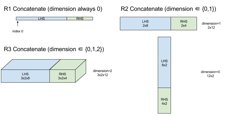
A concatenação compõe uma matriz de vários operandos. A matriz tem a mesma classificação de cada um dos operandos da matriz de entrada (que precisam ter a mesma classificação entre si) e contém os argumentos na ordem em que foram especificados.
Concatenate(operands..., dimension)
| Argumentos | Tipo | Semântica |
|---|---|---|
operands |
sequência de N XlaOp |
N matrizes do tipo T com dimensões [L0, L1, ...]. Requer N >= 1. |
dimension |
int64 |
Um valor no intervalo [0, N) que nomeia a dimensão a ser concatenada entre o operands. |
Com exceção de dimension, todas as dimensões precisam ser iguais. Isso ocorre
porque o XLA não é compatível com matrizes "arredondadas". Os valores de classificação 0 não podem ser concatenados, já que é impossível nomear a dimensão em que ocorre a concatenação.
Exemplo unidimensional:
Concat({ {2, 3}, {4, 5}, {6, 7} }, 0)
>>> {2, 3, 4, 5, 6, 7}
Exemplo de bidimensional:
let a = {
{1, 2},
{3, 4},
{5, 6},
};
let b = {
{7, 8},
};
Concat({a, b}, 0)
>>> {
{1, 2},
{3, 4},
{5, 6},
{7, 8},
}
Diagrama:
Condicional
Consulte também
XlaBuilder::Conditional.
Conditional(pred, true_operand, true_computation, false_operand,
false_computation)
| Argumentos | Tipo | Semântica |
|---|---|---|
pred |
XlaOp |
Escalar do tipo PRED |
true_operand |
XlaOp |
Argumento do tipo \(T_0\) |
true_computation |
XlaComputation |
XlaComputation do tipo \(T_0 \to S\) |
false_operand |
XlaOp |
Argumento do tipo \(T_1\) |
false_computation |
XlaComputation |
XlaComputation do tipo \(T_1 \to S\) |
Executa true_computation se pred for true, false_computation se pred
for false e retorna o resultado.
O true_computation precisa ter um único argumento do tipo \(T_0\) e será
invocado com true_operand, que precisa ser do mesmo tipo. O false_computation precisa ter um único argumento do tipo \(T_1\) e ser invocado com false_operand, que precisa ser do mesmo tipo. O tipo do
valor retornado de true_computation e false_computation precisa ser o mesmo.
Apenas um entre true_computation e false_computation será
executado, dependendo do valor de pred.
Conditional(branch_index, branch_computations, branch_operands)
| Argumentos | Tipo | Semântica |
|---|---|---|
branch_index |
XlaOp |
Escalar do tipo S32 |
branch_computations |
sequência de N XlaComputation |
XlaComputations do tipo \(T_0 \to S , T_1 \to S , ..., T_{N-1} \to S\) |
branch_operands |
sequência de N XlaOp |
Argumentos do tipo \(T_0 , T_1 , ..., T_{N-1}\) |
Executa branch_computations[branch_index] e retorna o resultado. Se
branch_index for um S32 < 0 ou >= N, branch_computations[N-1]
será executado como a ramificação padrão.
Cada branch_computations[b] precisa ter um único argumento do tipo \(T_b\) e
será invocado com branch_operands[b], que precisa ser do mesmo tipo. O
tipo do valor retornado de cada branch_computations[b] precisa ser o mesmo.
Apenas um dos branch_computations será executado, dependendo do
valor de branch_index.
Conv (convolução)
Consulte também
XlaBuilder::Conv.
Como ConvWithGeneralPadding, mas o padding é especificado resumidamente como SAME ou VÁLIDO. O MESMO padding preenche a entrada (lhs) com zeros para que
a saída tenha a mesma forma que a entrada quando não considerar
o salto. Padding VÁLIDO significa que não há padding.
ConvWithGeneralPadding (convolução)
Consulte também
XlaBuilder::ConvWithGeneralPadding.
Calcula uma convolução do tipo usado em redes neurais. Aqui, uma convolução pode ser considerada como uma janela de dimensão n que se move por uma área da base de dimensão n, e um cálculo é realizado para cada posição possível da janela.
| Argumentos | Tipo | Semântica |
|---|---|---|
lhs |
XlaOp |
Classificar matriz de entradas n+2 |
rhs |
XlaOp |
Classificar a matriz n+2 de pesos de kernel |
window_strides |
ArraySlice<int64> |
Matriz n-d de passos do kernel |
padding |
ArraySlice< pair<int64,int64>> |
Matriz n-d de padding (baixo, alto) |
lhs_dilation |
ArraySlice<int64> |
matriz de fator de dilatação de n-d lhs |
rhs_dilation |
ArraySlice<int64> |
matriz de fator de dilatação de n-d rhs |
feature_group_count |
int64 | o número de grupos de atributos |
batch_group_count |
int64 | o número de grupos em lote |
Permita que n seja o número de dimensões espaciais. O argumento lhs é uma matriz de classificação n+2 que descreve a área de base. Isso é chamado de entrada, embora,
claro, o rhs também seja uma entrada. Em uma rede neural, essas são as ativações de entrada.
As dimensões n+2 são, nesta ordem:
batch: cada coordenada nessa dimensão representa uma entrada independente em que a convolução é realizada.z/depth/features: cada posição (y,x) na área base tem um vetor associado a ela, que entra nessa dimensão.spatial_dims: descreve as dimensões espaciais donque definem a área de base em que a janela se move.
O argumento rhs é uma matriz de classificação n+2 que descreve o filtro/kernel/janela convolucional. As dimensões são, nesta ordem:
output-z: a dimensãozda saída.input-z: o tamanho dessa dimensão vezesfeature_group_countprecisa ser igual ao da dimensãoznas lhs.spatial_dims: descreve as dimensões espaciaisnque definem a janela "n-d", que se move pela área de base.
O argumento window_strides especifica o salto da janela convolucional
nas dimensões espaciais. Por exemplo, se o salto na primeira dimensão
espacial for 3, a janela só poderá ser colocada em coordenadas em que o
primeiro índice espacial seja divisível por 3.
O argumento padding especifica a quantidade de padding zero a ser aplicado à área de base. A quantidade de padding pode ser negativa. O valor absoluto do padding negativo indica o número de elementos que serão removidos da dimensão especificada antes da convolução. padding[0] especifica o padding da dimensão y, e padding[1] especifica o padding da dimensão x. Cada
par tem o padding baixo como o primeiro elemento e o padding alto como o segundo
elemento. O padding baixo é aplicado na direção dos índices mais baixos, enquanto o
alto é aplicado na direção dos índices mais altos. Por exemplo, se padding[1] for (2,3), haverá um padding por dois zeros à esquerda e três zeros à direita na segunda dimensão espacial. O uso de padding é equivalente a inserir esses mesmos valores zero na entrada (lhs) antes de fazer a convolução.
Os argumentos lhs_dilation e rhs_dilation especificam o fator de dilatação a ser aplicado a lhs e rhs, respectivamente, em cada dimensão espacial. Se o fator de dilatação em uma dimensão espacial for d, os buracos d-1 serão colocados implicitamente entre cada uma das entradas nessa dimensão, aumentando o tamanho da matriz. Os buracos são preenchidos com um valor de ambiente autônomo, o que significa zero para convolução.
A dilatação do rh também é chamada de convolução atrativa. Para mais detalhes, consulte
tf.nn.atrous_conv2d. A dilatação do lhs também é chamada de convolução
transposta. Confira mais detalhes em tf.nn.conv2d_transpose.
O argumento feature_group_count (valor padrão 1) pode ser usado para convoluções agrupadas. feature_group_count precisa ser um divisor da dimensão de entrada e
do atributo de saída. Se feature_group_count for maior que 1, significa que, conceitualmente, a dimensão do recurso de entrada e saída e a dimensão do recurso de saída rhs estão divididas igualmente em muitos grupos feature_group_count, cada um consistindo em uma subsequência consecutiva de recursos. A
dimensão de recurso de entrada de rhs precisa ser igual à dimensão do recurso de entrada
lhs dividida por feature_group_count. Assim, ela já tem o tamanho de um
grupo de recursos de entrada. Os grupos i-th são usados juntos para calcular feature_group_count para muitas convoluções separadas. Os resultados dessas convoluções são concatenados na dimensão de atributo de saída.
Para a convolução em profundidade, o argumento feature_group_count seria definido como a
dimensão de recurso de entrada e o filtro seria remodelado de
[filter_height, filter_width, in_channels, channel_multiplier] para
[filter_height, filter_width, 1, in_channels * channel_multiplier]. Para mais
detalhes, consulte tf.nn.depthwise_conv2d.
O argumento batch_group_count (valor padrão 1) pode ser usado para filtros agrupados
durante a retropropagação. batch_group_count precisa ser um divisor do tamanho da
dimensão de lote lhs (entrada). Se batch_group_count for maior
que 1, isso significa que a dimensão do lote de saída precisa ter o tamanho input batch
/ batch_group_count. O batch_group_count precisa ser um divisor do tamanho do recurso
de saída.
O formato de saída tem estas dimensões, nesta ordem:
batch: o tamanho dessa dimensão vezesbatch_group_countprecisa ser igual ao tamanho da dimensãobatchem lhs.z: mesmo tamanho queoutput-zno kernel (rhs).spatial_dims: um valor para cada posicionamento válido da janela convolucional.

A figura acima mostra como o campo batch_group_count funciona. Efetivamente, dividimos cada lote de lhs em grupos batch_group_count e fazemos o mesmo para os recursos de saída. Em seguida, para cada um desses grupos, fazemos convoluções entre pares e concatenamos a saída junto com a dimensão do atributo de saída. A semântica
operacional de todas as outras dimensões (recurso e espacial) permanece a mesma.
As posições válidas da janela convolucional são determinadas pelos passos e pelo tamanho da área de base após o preenchimento.
Para descrever o que uma convolução faz, considere uma convolução bidimensional e escolha algumas coordenadas fixas de batch, z, y e x na saída. (y,x) é a posição de um canto da janela dentro da área de base (por exemplo, o canto superior esquerdo, dependendo de como você interpreta as dimensões espaciais). Agora temos uma janela 2d, tirada da área de base, em que cada ponto 2d está associado a um vetor 1d, então temos uma caixa 3d. No kernel convolucional, como corrigimos a coordenada de saída z, também temos uma caixa 3D. As duas caixas têm as mesmas
dimensões, então podemos pegar a soma dos produtos com elementos entre as duas
caixas (semelhante a um produto escalar). Esse é o valor de saída.
Observe que, se output-z for, por exemplo, 5, cada posição da janela produzirá cinco
valores na saída para a dimensão z da saída. Esses valores diferem
em que parte do kernel convolucional é usada. Há uma caixa 3D separada de
valores usados para cada coordenada output-z. Você pode pensar nisso como cinco convoluções separadas, com um filtro diferente para cada uma delas.
Este é um pseudocódigo para uma convolução 2D com padding e strido:
for (b, oz, oy, ox) {  // output coordinates
  value = 0;
  for (iz, ky, kx) {  // kernel coordinates and input z
    iy = oy*stride_y + ky - pad_low_y;
    ix = ox*stride_x + kx - pad_low_x;
    if ((iy, ix) inside the base area considered without padding) {
      value += input(b, iz, iy, ix) * kernel(oz, iz, ky, kx);
    }
  }
  output(b, oz, oy, ox) = value;
}
ConvertElementType
Consulte também
XlaBuilder::ConvertElementType.
De forma semelhante a uma static_cast com elementos em C++, executa uma operação de conversão
de elemento de uma forma de dados para um formato de destino. As dimensões precisam ser
correspondentes, e a conversão é precisa de elementos. Por exemplo, os elementos s32 se tornam elementos
f32 usando uma rotina de conversão de s32 para f32.
ConvertElementType(operand, new_element_type)
| Argumentos | Tipo | Semântica |
|---|---|---|
operand |
XlaOp |
matriz do tipo T com escurecimento D |
new_element_type |
PrimitiveType |
tipo U |
As dimensões do operando e o formato de destino precisam ser iguais. Os tipos de elemento de origem e destino não podem ser tuplas.
Uma conversão como T=s32 para U=f32 vai executar uma rotina de conversão "int-to-float" de normalização, como "arredondar para mais próximo".
let a: s32[3] = {0, 1, 2};
let b: f32[3] = convert(a, f32);
then b == f32[3]{0.0, 1.0, 2.0}
CrossReplicaSum
Executa AllReduce com um cálculo de soma.
CustomCall
Consulte também
XlaBuilder::CustomCall.
Chamar uma função fornecida pelo usuário em um cálculo.
CustomCall(target_name, args..., shape)
| Argumentos | Tipo | Semântica |
|---|---|---|
target_name |
string |
Nome da função. Será emitida uma instrução de chamada direcionada a esse nome de símbolo. |
args |
sequência de N XlaOps |
N argumentos de tipo arbitrário, que serão transmitidos para a função. |
shape |
Shape |
Forma de saída da função |
A assinatura da função é a mesma, independentemente da arity ou do tipo de argumentos:
extern "C" void target_name(void* out, void** in);
Por exemplo, se CustomCall for usado da seguinte maneira:
let x = f32[2] {1,2};
let y = f32[2x3] { {10, 20, 30}, {40, 50, 60} };

CustomCall("myfunc", {x, y}, f32[3x3])
Confira um exemplo de implementação de myfunc:
extern "C" void myfunc(void* out, void** in) {
  float (&x)[2] = *static_cast<float(*)[2]>(in[0]);
  float (&y)[2][3] = *static_cast<float(*)[2][3]>(in[1]);
  EXPECT_EQ(1, x[0]);
  EXPECT_EQ(2, x[1]);
  EXPECT_EQ(10, y[0][0]);
  EXPECT_EQ(20, y[0][1]);
  EXPECT_EQ(30, y[0][2]);
  EXPECT_EQ(40, y[1][0]);
  EXPECT_EQ(50, y[1][1]);
  EXPECT_EQ(60, y[1][2]);
  float (&z)[3][3] = *static_cast<float(*)[3][3]>(out);
  z[0][0] = x[1] + y[1][0];
  // ...
}
A função fornecida pelo usuário não pode ter efeitos colaterais, e a execução dela precisa ser idempotente.
Dot
Consulte também
XlaBuilder::Dot.
Dot(lhs, rhs)
| Argumentos | Tipo | Semântica |
|---|---|---|
lhs |
XlaOp |
matriz do tipo T |
rhs |
XlaOp |
matriz do tipo T |
A semântica exata dessa operação depende das classificações dos operandos:
| Entrada | Saída | Semântica |
|---|---|---|
vetor [n] dot vetor [n] |
escalar | produto escalar vetorial |
matriz [m x k] dot vetor [k] |
vetor [m] | multiplicação de vetores de matriz |
matriz [m x k] dot matriz [k x n] |
matriz [m x n] | multiplicação matricial |
A operação executa a soma dos produtos sobre a segunda dimensão de lhs (ou
a primeira, se tiver classificação 1) e a primeira dimensão de rhs. Essas são as dimensões "contratadas". As dimensões contratadas de lhs e rhs precisam ser do mesmo tamanho. Na prática, ela pode ser usada para realizar produtos escalares entre vetores, multiplicações de vetor/matriz ou multiplicações de matriz/matriz.
DotGeneral
Consulte também
XlaBuilder::DotGeneral.
DotGeneral(lhs, rhs, dimension_numbers)
| Argumentos | Tipo | Semântica |
|---|---|---|
lhs |
XlaOp |
matriz do tipo T |
rhs |
XlaOp |
matriz do tipo T |
dimension_numbers |
DotDimensionNumbers |
contratações e números de dimensão de lote |
Semelhante ao ponto, mas permite que os números de dimensão de contrato e lote sejam
especificados para lhs e rhs.
| Campos DotDimensionNumbers | Tipo | Semântica |
|---|---|---|
lhs_contracting_dimensions
|
int64 repetido | lhs números de dimensões de
contração |
rhs_contracting_dimensions
|
int64 repetido | rhs números de dimensões de
contração |
lhs_batch_dimensions
|
int64 repetido | lhs número da dimensão do lote |
rhs_batch_dimensions
|
int64 repetido | rhs número da dimensão do lote |
O DotGeneral executa a soma dos produtos sobre as dimensões de contrato especificadas em
dimension_numbers.
Os números de dimensão de contratação associados de lhs e rhs não precisam ser os mesmos, mas precisam ter os mesmos tamanhos de dimensão.
Exemplo com números de dimensão contratantes:
lhs = { {1.0, 2.0, 3.0},
{4.0, 5.0, 6.0} }

rhs = { {1.0, 1.0, 1.0},
{2.0, 2.0, 2.0} }

DotDimensionNumbers dnums;
dnums.add_lhs_contracting_dimensions(1);
dnums.add_rhs_contracting_dimensions(1);

DotGeneral(lhs, rhs, dnums) -> { {6.0, 12.0},
{15.0, 30.0} }
Os números de dimensão de lote associados de lhs e rhs precisam ter os mesmos
tamanhos de dimensão.
Exemplo com números de dimensão de lote (tamanho de lote 2, matrizes 2x2):
lhs = { { {1.0, 2.0},
{3.0, 4.0} },
{ {5.0, 6.0},
{7.0, 8.0} } }

rhs = { { {1.0, 0.0},
{0.0, 1.0} },
{ {1.0, 0.0},
{0.0, 1.0} } }

DotDimensionNumbers dnums;
dnums.add_lhs_contracting_dimensions(2);
dnums.add_rhs_contracting_dimensions(1);
dnums.add_lhs_batch_dimensions(0);
dnums.add_rhs_batch_dimensions(0);

DotGeneral(lhs, rhs, dnums) -> { { {1.0, 2.0},
{3.0, 4.0} },
{ {5.0, 6.0},
{7.0, 8.0} } }
| Entrada | Saída | Semântica |
|---|---|---|
[b0, m, k] dot [b0, k, n] |
[b0, m, n] | Batch matmul |
[b0, b1, m, k] dot [b0, b1, k, n] |
[b0, b1, m, n] | Batch matmul |
O número de dimensão resultante começa com a dimensão do lote, depois a dimensão lhs sem contrato/sem lote e, por fim, a dimensão rhs não contratante/sem lote.
DynamicSlice
Consulte também
XlaBuilder::DynamicSlice.
DynamicSlice extrai uma submatriz da matriz de entrada na start_indices dinâmica. O tamanho da fração em cada dimensão é transmitido em
size_indices, que especifica o ponto final dos intervalos exclusivos de frações em cada
dimensão: [início, início + tamanho). O formato de start_indices precisa ser de classificação ==
1, com o tamanho da dimensão igual à classificação de operand.
DynamicSlice(operand, start_indices, size_indices)
| Argumentos | Tipo | Semântica |
|---|---|---|
operand |
XlaOp |
Matriz dimensional N do tipo T |
start_indices |
sequência de N XlaOp |
Lista de N números inteiros escalares que contêm os índices iniciais da fatia de cada dimensão. O valor precisa ser maior ou igual a zero. |
size_indices |
ArraySlice<int64> |
Lista de N números inteiros com o tamanho da fatia de cada dimensão. Cada valor precisa ser estritamente maior do que zero, e start + size precisa ser menor ou igual ao tamanho da dimensão para evitar quebrar o tamanho da dimensão do módulo. |
Os índices de frações efetivas são calculados aplicando a seguinte transformação para cada índice i em [1, N) antes de executar a fração:
start_indices[i] = clamp(start_indices[i], 0, operand.dimension_size[i] - size_indices[i])
Isso garante que a fração extraída esteja sempre dentro dos limites em relação à matriz de operandos. Se a fração estiver dentro dos limites antes da aplicação da transformação, a transformação não terá efeito.
Exemplo unidimensional:
let a = {0.0, 1.0, 2.0, 3.0, 4.0}
let s = {2}

DynamicSlice(a, s, {2}) produces:
{2.0, 3.0}
Exemplo de bidimensional:
let b =
{ {0.0,  1.0,  2.0},
{3.0,  4.0,  5.0},
{6.0,  7.0,  8.0},
{9.0, 10.0, 11.0} }
let s = {2, 1}

DynamicSlice(b, s, {2, 2}) produces:
{ { 7.0,  8.0},
{10.0, 11.0} }
DynamicUpdateSlice
Consulte também
XlaBuilder::DynamicUpdateSlice.
DynamicUpdateSlice gera um resultado que é o valor da matriz de entrada operand, com uma fração update substituída em start_indices.
A forma de update determina o formato da submatriz do resultado que
é atualizado.
A forma de start_indices precisa ter classificação == 1, com o tamanho da dimensão igual à
classificação de operand.
DynamicUpdateSlice(operand, update, start_indices)
| Argumentos | Tipo | Semântica |
|---|---|---|
operand |
XlaOp |
Matriz dimensional N do tipo T |
update |
XlaOp |
Matriz dimensional N do tipo T contendo a atualização da fatia. Cada dimensão do formato de atualização precisa ser estritamente maior que zero, e start + update precisa ser menor ou igual ao tamanho do operando para cada dimensão para evitar a geração de índices de atualização fora dos limites. |
start_indices |
sequência de N XlaOp |
Lista de N números inteiros escalares que contêm os índices iniciais da fatia de cada dimensão. O valor precisa ser maior ou igual a zero. |
Os índices de frações efetivas são calculados aplicando a seguinte transformação para cada índice i em [1, N) antes de executar a fração:
start_indices[i] = clamp(start_indices[i], 0, operand.dimension_size[i] - update.dimension_size[i])
Isso garante que a fração atualizada esteja sempre dentro dos limites em relação à matriz de operandos. Se a fração estiver dentro dos limites antes da aplicação da transformação, a transformação não terá efeito.
Exemplo unidimensional:
let a = {0.0, 1.0, 2.0, 3.0, 4.0}
let u = {5.0, 6.0}
let s = {2}

DynamicUpdateSlice(a, u, s) produces:
{0.0, 1.0, 5.0, 6.0, 4.0}
Exemplo de bidimensional:
let b =
{ {0.0,  1.0,  2.0},
{3.0,  4.0,  5.0},
{6.0,  7.0,  8.0},
{9.0, 10.0, 11.0} }
let u =
{ {12.0,  13.0},
{14.0,  15.0},
{16.0,  17.0} }

let s = {1, 1}

DynamicUpdateSlice(b, u, s) produces:
{ {0.0,  1.0,  2.0},
{3.0, 12.0, 13.0},
{6.0, 14.0, 15.0},
{9.0, 16.0, 17.0} }
Operações aritméticas binárias por elemento
Consulte também
XlaBuilder::Add.
Há suporte para um conjunto de operações aritméticas binárias de elemento por elemento.
Op(lhs, rhs)
Em que Op é Add (adição), Sub (subtração), Mul
(multiplicação), Div (divisão), Rem (restante), Max (máximo), Min
(mínimo), LogicalAnd (AND lógico) ou LogicalOr (OR lógico).
| Argumentos | Tipo | Semântica |
|---|---|---|
lhs |
XlaOp |
Operando do lado esquerdo: matriz do tipo T |
rhs |
XlaOp |
Operando do lado direito: matriz do tipo T |
As formas dos argumentos precisam ser semelhantes ou compatíveis. Consulte a documentação sobre transmissão sobre o que significa que as formas são compatíveis. O resultado de uma operação tem uma forma, que é resultado da transmissão das duas matrizes de entrada. Nessa variante, as operações entre matrizes de classificações diferentes não são compatíveis, a menos que um dos operandos seja um escalar.
Quando Op é Rem, o sinal do resultado é retirado do dividendo, e o
valor absoluto do resultado é sempre menor que o valor absoluto do divisor.
O estouro de divisão de números inteiros (divisão/restrito assinado/não assinado por zero ou
divisão/restante assinado de INT_SMIN com -1) produz um valor definido pela
implementação.
Existe uma variante alternativa com suporte à transmissão de classificações diferentes para estas operações:
Op(lhs, rhs, broadcast_dimensions)
Em que Op é igual ao exemplo acima. Essa variante da operação precisa ser usada
para operações aritméticas entre matrizes de classificações diferentes (como adicionar uma
matriz a um vetor).
O operando de classificação broadcast_dimensions adicional é uma fração de números inteiros usada para
expandir a classificação do operando de classificação inferior até a classificação do operando de
classificação mais alta. broadcast_dimensions mapeia as dimensões da forma de classificação inferior para as dimensões do formato de classificação superior. As dimensões não mapeadas da forma expandida
são preenchidas com dimensões de tamanho um. A transmissão de dimensão desgenerada
transmite as formas ao longo dessas dimensões para equalizar as
formas dos dois operandos. A semântica é descrita em detalhes na
página de transmissão.
Operações de comparação por elemento
Consulte também
XlaBuilder::Eq.
Há suporte para um conjunto de operações de comparação binária de elemento padrão padrão. Observe que a semântica padrão de comparação de ponto flutuante IEEE 754 se aplica ao comparar tipos de ponto flutuante.
Op(lhs, rhs)
Em que Op é Eq (igual a), Ne (diferente de), Ge
(maior ou igual a), Gt (maior que), Le (menor ou igual a), Lt
(menor que). Outro conjunto de operadores, EqTotalOrder, NeTotalOrder, GeTotalOrder,
GtTotalOrder, LeTotalOrder e LtTotalOrder, fornece as mesmas funcionalidades,
exceto que também são compatíveis com um pedido total sobre os números de pontos
flutuantes, aplicando -NaN < -Inf < -Finite < -0 < +0 < +Finite < +N.
| Argumentos | Tipo | Semântica |
|---|---|---|
lhs |
XlaOp |
Operando do lado esquerdo: matriz do tipo T |
rhs |
XlaOp |
Operando do lado direito: matriz do tipo T |
As formas dos argumentos precisam ser semelhantes ou compatíveis. Consulte a documentação sobre transmissão sobre o que significa que as formas são compatíveis. O resultado de uma operação tem uma forma, que é o resultado da transmissão das duas matrizes de entrada com o tipo de elemento PRED. Nessa variante,
as operações entre matrizes de classificações diferentes não são compatíveis, a menos que um
dos operandos seja um escalar.
Existe uma variante alternativa com suporte à transmissão de classificações diferentes para estas operações:
Op(lhs, rhs, broadcast_dimensions)
Em que Op é igual ao exemplo acima. Essa variante da operação precisa ser usada
para operações de comparação entre matrizes de classificações diferentes (como adicionar uma
matriz a um vetor).
O operando adicional broadcast_dimensions é uma fração de números inteiros que especifica
as dimensões a serem usadas para transmitir os operandos. A semântica é descrita
em detalhes na página de transmissão.
Funções unárias por elementos
O XlaBuilder oferece suporte a estas funções unárias de elemento:
Abs(operand) Abs x -> |x| por elemento.
Ceil(operand) Ceil por elemento x -> ⌈x⌉.
Cos(operand) Cosseno por elemento x -> cos(x).
Exp(operand) Exponencial natural por elemento x -> e^x.
Floor(operand) Valor mínimo x -> ⌊x⌋.
Imag(operand) Parte imaginária com elementos de uma forma complexa (ou real). x -> imag(x). Se o operando for um tipo de ponto flutuante, retorna 0.
IsFinite(operand) Testa se cada elemento de operand é finito,
ou seja, não é um infinito positivo ou negativo e não é NaN. Retorna uma matriz de valores PRED com a mesma forma da entrada, em que cada elemento será true somente se o elemento de entrada correspondente for finito.
Log(operand) Logaritmo natural de elemento x -> ln(x).
LogicalNot(operand) Lógica por elemento não x -> !(x).
Logistic(operand) Computação da função logística por elementos x ->
logistic(x).
PopulationCount(operand) Calcula o número de bits definidos em cada
elemento de operand.
Neg(operand) Negação por elemento x -> -x.
Real(operand) Parte real por elementos de uma forma complexa (ou real).
x -> real(x). Se o operando for um tipo de ponto flutuante, retorna o mesmo valor.
Rsqrt(operand) Recíproco por elemento da operação de raiz quadrada
x -> 1.0 / sqrt(x).
Sign(operand) Operação de sinal por elemento x -> sgn(x) em que
\[\text{sgn}(x) = \begin{cases} -1 & x < 0\\ -0 & x = -0\\ NaN & x = NaN\\ +0 & x = +0\\ 1 & x > 0 \end{cases}\]
usando o operador de comparação do tipo de elemento de operand.
Sqrt(operand) Operação de raiz quadrada por elemento x -> sqrt(x).
Cbrt(operand) Operação de raiz cúbica por elemento x -> cbrt(x).
Tanh(operand) Tangente hiperbólica por elemento x -> tanh(x).
Round(operand) Arredondamento por elemento, empates fora de zero.
RoundNearestEven(operand) Arredondamento por elemento, associa ao par mais próximo.
| Argumentos | Tipo | Semântica |
|---|---|---|
operand |
XlaOp |
O operando para a função |
A função é aplicada a cada elemento na matriz operand, resultando em uma matriz com o mesmo formato. operand pode ser um escalar (classificação 0).
Fft
A operação FFT do XLA implementa as Transforms Fourier direta e inversa para entradas/saídas reais e complexas. Há suporte para FFTs multidimensionais em até três eixos.
Consulte também
XlaBuilder::Fft.
| Argumentos | Tipo | Semântica |
|---|---|---|
operand |
XlaOp |
A matriz que estamos transformando Fourier. |
fft_type |
FftType |
Consulte a tabela abaixo. |
fft_length |
ArraySlice<int64> |
Os comprimentos de domínio de tempo dos eixos que estão sendo transformados. Isso é necessário principalmente para que a IRFFT dimensione corretamente o eixo mais interno, já que RFFT(fft_length=[16]) tem a mesma forma de saída que RFFT(fft_length=[17]) |
FftType |
Semântica |
|---|---|
FFT |
Encaminhar FFT complexo para complexo. A forma não foi alterada. |
IFFT |
Inversa de FFT complexa para complexa. A forma não foi alterada. |
RFFT |
Encaminhar FFT real para complexo. A forma do eixo mais interno é reduzida a fft_length[-1] // 2 + 1 se fft_length[-1] for um valor diferente de zero, omitindo a parte conjugada invertida do sinal transformado além da frequência Nyquist. |
IRFFT |
Inversão da FFT real para complexa (ou seja, toma complexidade, retorna real). A forma do eixo mais interno vai ser expandida para fft_length[-1] se fft_length[-1] for um valor diferente de zero, deduzindo a parte do sinal transformado além da frequência Nyquist do conjugado reverso das entradas 1 para fft_length[-1] // 2 + 1. |
FFT multidimensional
Quando mais de um fft_length é fornecido, isso equivale a aplicar uma cascata de operações FFT a cada um dos eixos mais internos. Observe que, para os casos reais, complexos e complexos, a transformação do eixo mais interno é realizada primeiro (RFFT; por último para IRFFT), e é por isso que o eixo mais interno é o que muda de tamanho. Outras transformações de eixo serão então
complexas -> complexas.
Detalhes da implementação
A FFT da CPU usa o TensorFFT do Eigen. A GPU FFT usa cuFFT.
Gather
A operação de coleta do XLA une várias fatias de uma matriz de entrada, cada uma em um deslocamento de ambiente de execução potencialmente diferente.
Semântica geral
Consulte também
XlaBuilder::Gather.
Para uma descrição mais intuitiva, consulte a seção "Descrição informativa" abaixo.
gather(operand, start_indices, offset_dims, collapsed_slice_dims, slice_sizes, start_index_map)
| Argumentos | Tipo | Semântica |
|---|---|---|
operand |
XlaOp |
A matriz da qual estamos coletando. |
start_indices |
XlaOp |
Matriz contendo os índices iniciais das fatias coletadas. |
index_vector_dim |
int64 |
A dimensão em start_indices que "contém" os índices iniciais. Veja abaixo uma descrição detalhada. |
offset_dims |
ArraySlice<int64> |
O conjunto de dimensões na forma de saída que se deslocam em uma matriz cortada do operando. |
slice_sizes |
ArraySlice<int64> |
slice_sizes[i] são os limites para a fatia na dimensão i. |
collapsed_slice_dims |
ArraySlice<int64> |
O conjunto de dimensões em cada fatia que são recolhidas. Essas dimensões precisam ter o tamanho 1. |
start_index_map |
ArraySlice<int64> |
Um mapa que descreve como mapear índices em start_indices para índices legais no operando. |
indices_are_sorted |
bool |
Indica se os índices serão classificados pelo autor da chamada. |
unique_indices |
bool |
Se os índices têm garantia de serem exclusivos pelo autor da chamada. |
Por conveniência, rotulamos as dimensões na matriz de saída como batch_dims
que não estão em offset_dims.
O resultado é uma matriz de classificação batch_dims.size + offset_dims.size.
O operand.rank precisa ser igual à soma de offset_dims.size e
collapsed_slice_dims.size. Além disso, slice_sizes.size precisa ser igual a
operand.rank.
Se index_vector_dim for igual a start_indices.rank, vamos considerar implicitamente
start_indices como uma dimensão 1 à direita. Ou seja, se start_indices estava na
forma [6,7] e index_vector_dim for 2, vamos considerar implicitamente start_indices como [6,7,1].
Os limites para a matriz de saída na dimensão i são calculados da seguinte maneira:
Se
iestiver presente embatch_dims(ou seja, for igual abatch_dims[k]para algunsk), vamos escolher os limites de dimensão correspondentes destart_indices.shape, pulandoindex_vector_dim(ou seja, escolhastart_indices.shape.dims[k] sek<index_vector_dimestart_indices.shape.dims[k+1] caso contrário).Se
iestiver presente emoffset_dims(ou seja, igual aoffset_dims[k] para algunsk), vamos escolher o limite correspondente deslice_sizesapós contabilizarcollapsed_slice_dims(ou seja, escolhemosadjusted_slice_sizes[k] em queadjusted_slice_sizeséslice_sizescom os limites nos índices decollapsed_slice_dimsremovidos).
Formalmente, o índice de operando In correspondente a um determinado índice de saída Out é
calculado da seguinte maneira:
Permita que
G= {Out[k] parakembatch_dims}. UseGpara separar um vetorSde modo queS[i] =start_indices[Combine(G,i)] em que Combine(A, b) insira b na posiçãoindex_vector_dimem A. Isso é bem definido mesmo queGesteja vazio: seGestiver vazio,S=start_indices.Crie um índice inicial,
Sin, emoperandusandoSdistribuindoScomstart_index_map. Mais precisão:Sin[start_index_map[k]] =S[k] sek<start_index_map.size.Sin[_] =0.
Crie um índice
Oinemoperandespalhando os índices nas dimensões de deslocamento emOutde acordo com o conjunto decollapsed_slice_dims. Mais precisão:Oin[remapped_offset_dims(k)] =Out[offset_dims[k]] sek<offset_dims.size(remapped_offset_dimsé definido abaixo).Oin[_] =0.
InéOin+Sin, em que + é uma adição de elemento.
remapped_offset_dims é uma função monotônica com domínio [0,
offset_dims.size) e intervalo [0, operand.rank) \ collapsed_slice_dims. Então,
se, por exemplo, offset_dims.size é 4, operand.rank é 6 e
collapsed_slice_dims é {0, 2}, então remapped_offset_dims é {0→1,
1→3, 2→4, 3→5}.
Se indices_are_sorted for definido como verdadeiro, o XLA poderá presumir que start_indices
são classificados (em ordem crescente de start_index_map) pelo usuário. Se não forem, a semântica será implementada.
Se unique_indices for definido como verdadeiro, o XLA poderá presumir que todos os elementos
dispersos são exclusivos. Portanto, o XLA pode usar operações não atômicas. Se
unique_indices for definido como verdadeiro e os índices que estão sendo dispersos não forem
exclusivos, a semântica será implementada.
Descrição informal e exemplos
informalmente, cada índice Out na matriz de saída corresponde a um elemento E
na matriz de operandos, calculado da seguinte maneira:
Usamos as dimensões do lote em
Outpara procurar um índice inicial destart_indices.Usamos
start_index_mappara mapear o índice inicial (cujo tamanho pode ser menor que opera.rank) para um índice inicial "completo" nooperand.Cortamos uma fração com o tamanho
slice_sizesusando o índice inicial completo.Para remodelar a fatia, recolhe as dimensões
collapsed_slice_dims. Como todas as dimensões das fatias recolhidas precisam ter um limite de 1, essa remodelação é sempre legal.Usamos as dimensões de deslocamento em
Outpara indexar essa fração e conseguir o elemento de entrada,E, correspondente ao índice de saídaOut.
index_vector_dim está definido como start_indices.rank - 1 em todos os exemplos
a seguir. Valores mais interessantes para index_vector_dim não alteram a
operação fundamentalmente, mas tornam a representação visual mais complicada.
Para ter uma ideia de como os itens acima se encaixam, vejamos um
exemplo que reúne cinco fatias da forma [8,6] de uma matriz [16,11]. A posição de uma fração na matriz [16,11] pode ser representada como um vetor de índice da forma S64[2], portanto, o conjunto de cinco posições pode ser representado como uma matriz S64[5,2].
O comportamento da operação de coleta pode ser representado como uma transformação
de índice que usa [G,O0,O1], um índice na
forma de saída, e o associa a um elemento na matriz de entrada desta
maneira:

Primeiro, selecionamos um vetor (X,Y) da matriz de índices de agrupamento usando G.
O elemento na matriz de saída no índice [G,O0,O1] é, então, o elemento na matriz de entrada no índice [X+O0,Y+O1].
slice_sizes é [8,6], que decide o intervalo de O0 e
O1 e, por sua vez, decide os limites da fatia.
Essa operação de coleta atua como uma fração dinâmica de lote com G como a dimensão
do lote.
Os índices de coleta podem ser multidimensionais. Por exemplo, uma versão mais geral do exemplo acima usando uma matriz de "índices de coleta" da forma [4,5,2] traduziria índices como este:

Novamente, isso age como uma fração dinâmica de lote G0 e
G1 como as dimensões do lote. O tamanho da fatia ainda é [8,6].
A operação de coleta em XLA generaliza a semântica informal descrita acima das seguintes maneiras:
Podemos configurar quais dimensões na forma de saída são as dimensões de deslocamento (dimensões contendo
O0,O1no último exemplo). As dimensões do lote de saída (dimensões que contêmG0,G1no último exemplo) são definidas como as dimensões de saída que não são dimensões de deslocamento.O número de dimensões de deslocamento de saída explicitamente presentes no formato de saída pode ser menor do que a classificação de entrada. Essas dimensões "ausentes", que estão listadas explicitamente como
collapsed_slice_dims, precisam ter um tamanho de fatia1. Como eles têm um tamanho de fatia de1, o único índice válido para eles é0e escondê-los não gera ambiguidade.A fração extraída da matriz "Gather Indices" ((
X,Y) no último exemplo) pode ter menos elementos do que a classificação da matriz de entrada. Um mapeamento explícito dita como o índice precisa ser expandido para ter a mesma classificação que a entrada.
Como exemplo final, usamos (2) e (3) para implementar tf.gather_nd:

G0 e G1 são usados para separar um índice inicial
da matriz de índices de coleta como de costume, com a exceção de que o índice inicial tem apenas um
elemento, X. Da mesma forma, há apenas um índice de deslocamento de saída com o valor
O0. No entanto, antes de serem usados como índices na matriz de entrada,
eles são expandidos de acordo com "Gather Index Mapping" (start_index_map na
descrição formal) e "Offset Mapping" (remapped_offset_dims na
descrição formal) em [X,0] e [0,O0],
respectivamente, somando [X,O0]. Em outras palavras, o índice de saída
[G0,G, o índice de saída
[G0,G] para a semântica, como input
[G0,G].00OO11GatherIndicestf.gather_nd
O slice_sizes neste caso é [1,11]. Intuitivamente, isso significa que cada X de índice na matriz de índices de coleta escolhe uma linha inteira, e o resultado é a concatenação de todas essas linhas.
GetDimensionSize
Consulte também
XlaBuilder::GetDimensionSize.
Retorna o tamanho da dimensão especificada do operando. O operando precisa ter formato de matriz.
GetDimensionSize(operand, dimension)
| Argumentos | Tipo | Semântica |
|---|---|---|
operand |
XlaOp |
matriz de entrada dimensional n |
dimension |
int64 |
Um valor no intervalo [0, n) que especifica a dimensão |
SetDimensionSize
Consulte também
XlaBuilder::SetDimensionSize.
Define o tamanho dinâmico da dimensão especificada do XlaOp. O operando precisa ter formato de matriz.
SetDimensionSize(operand, size, dimension)
| Argumentos | Tipo | Semântica |
|---|---|---|
operand |
XlaOp |
matriz de entrada dimensional n. |
size |
XlaOp |
int32 representando o tamanho dinâmico do ambiente de execução. |
dimension |
int64 |
Um valor no intervalo [0, n) que especifica a dimensão. |
Transmita pelo operando como resultado, com a dimensão dinâmica rastreada pelo compilador.
Os valores preenchidos serão ignorados pelas operações de redução downstream.
let v: f32[10] = f32[10]{1, 2, 3, 4, 5, 6, 7, 8, 9, 10};
let five: s32 = 5;
let six: s32 = 6;

// Setting dynamic dimension size doesn't change the upper bound of the static
// shape.
let padded_v_five: f32[10] = set_dimension_size(v, five, /*dimension=*/0);
let padded_v_six: f32[10] = set_dimension_size(v, six, /*dimension=*/0);

// sum == 1 + 2 + 3 + 4 + 5
let sum:f32[] = reduce_sum(padded_v_five);
// product == 1 * 2 * 3 * 4 * 5
let product:f32[] = reduce_product(padded_v_five);

// Changing padding size will yield different result.
// sum == 1 + 2 + 3 + 4 + 5 + 6
let sum:f32[] = reduce_sum(padded_v_six);
GetTupleElement
Consulte também
XlaBuilder::GetTupleElement.
Índices em uma tupla com um valor de constante de tempo de compilação.
O valor precisa ser uma constante de tempo de compilação para que a inferência de forma possa determinar o tipo do valor resultante.
Isso é análogo a std::get<int N>(t) em C++. Conceitualmente:
let v: f32[10] = f32[10]{0, 1, 2, 3, 4, 5, 6, 7, 8, 9};
let s: s32 = 5;
let t: (f32[10], s32) = tuple(v, s);
let element_1: s32 = gettupleelement(t, 1);  // Inferred shape matches s32.
Consulte também tf.tuple.
Entrada
Consulte também
XlaBuilder::Infeed.
Infeed(shape)
| Argumento | Tipo | Semântica |
|---|---|---|
shape |
Shape |
Forma dos dados lidos da interface de Infeed. O campo de layout da forma precisa ser definido para corresponder ao layout dos dados enviados ao dispositivo. Caso contrário, o comportamento será indefinido. |
Lê um único item de dados na interface de streaming de entrada implícita do dispositivo, interpretando os dados como a forma e o layout especificados e retorna um XlaOp dos dados. Várias operações de entrada são permitidas em um cálculo, mas deve haver um pedido total entre as operações de entrada. Por exemplo, dois Infeeds no código abaixo têm uma ordem total, já que há uma dependência entre os loops "while".
result1 = while (condition, init = init_value) {
  Infeed(shape)
}

result2 = while (condition, init = result1) {
  Infeed(shape)
}
Formas de tuplas aninhadas não são aceitas. Para uma forma de tupla vazia, a operação de entrada é efetivamente um ambiente autônomo e prossegue sem ler nenhum dado da entrada do dispositivo.
Iota
Consulte também
XlaBuilder::Iota.
Iota(shape, iota_dimension)
Cria um literal constante no dispositivo em vez de uma transferência de host potencialmente grande. Cria uma matriz com uma forma especificada e mantém valores a partir de zero que incrementam em um ao longo da dimensão especificada. Para tipos de
ponto flutuante, a matriz produzida é equivalente a ConvertElementType(Iota(...)), em que
o Iota é do tipo integral e a conversão é para o tipo de ponto flutuante.
| Argumentos | Tipo | Semântica |
|---|---|---|
shape |
Shape |
Forma da matriz criada por Iota() |
iota_dimension |
int64 |
A dimensão a ser incrementada. |
Por exemplo, Iota(s32[4, 8], 0) retorna
  [[0, 0, 0, 0, 0, 0, 0, 0 ],
   [1, 1, 1, 1, 1, 1, 1, 1 ],
   [2, 2, 2, 2, 2, 2, 2, 2 ],
   [3, 3, 3, 3, 3, 3, 3, 3 ]]
Devolução por Iota(s32[4, 8], 1)
  [[0, 1, 2, 3, 4, 5, 6, 7 ],
   [0, 1, 2, 3, 4, 5, 6, 7 ],
   [0, 1, 2, 3, 4, 5, 6, 7 ],
   [0, 1, 2, 3, 4, 5, 6, 7 ]]
Mapa
Consulte também
XlaBuilder::Map.
Map(operands..., computation)
| Argumentos | Tipo | Semântica |
|---|---|---|
operands |
sequência de N XlaOps |
N matrizes dos tipos T0..T{N-1} |
computation |
XlaComputation |
Computação do tipo T_0, T_1, .., T_{N + M -1} -> S com N parâmetros do tipo T e M do tipo arbitrário |
dimensions |
Matriz int64 |
matriz de dimensões de mapa |
Aplica uma função escalar sobre as matrizes operands especificadas, produzindo uma matriz das mesmas dimensões, em que cada elemento é o resultado da função mapeada aplicada aos elementos correspondentes nas matrizes de entrada.
A função mapeada é um cálculo arbitrário com a restrição de que tem N entradas do tipo escalar T e uma única saída com o tipo S. A saída tem
as mesmas dimensões que os operandos, mas o tipo de elemento T é substituído
por S.
Por exemplo: Map(op1, op2, op3, computation, par1) mapeia elem_out <-
computation(elem1, elem2, elem3, par1) em cada índice (multidimensional) nas matrizes de entrada para produzir a matriz de saída.
OptimizationBarrier
Impede que qualquer passe de otimização mova os cálculos pela barreira.
Garante que todas as entradas sejam avaliadas antes de qualquer operador que dependa das saídas da barreira.
Adesivo
Consulte também
XlaBuilder::Pad.
Pad(operand, padding_value, padding_config)
| Argumentos | Tipo | Semântica |
|---|---|---|
operand |
XlaOp |
matriz do tipo T |
padding_value |
XlaOp |
escalar do tipo T para preencher o padding adicionado |
padding_config |
PaddingConfig |
valor de padding nas duas bordas (baixo, alto) e entre os elementos de cada dimensão |
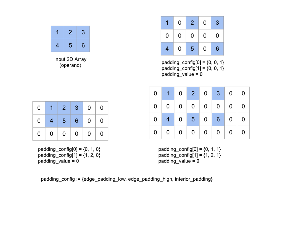
Expande a matriz operand especificada preenchendo a matriz e entre os elementos com o padding_value especificado. padding_config
especifica a quantidade de padding da borda e do padding interno para cada
dimensão.
PaddingConfig é um campo repetido de PaddingConfigDimension, que contém três campos para cada dimensão: edge_padding_low, edge_padding_high e interior_padding.
edge_padding_low e edge_padding_high especificam a quantidade de padding adicionada
na parte inferior (ao lado do índice 0) e na parte sofisticada (ao lado do índice mais alto) de
cada dimensão, respectivamente. O padding da borda pode ser negativo. O valor absoluto do padding negativo indica o número de elementos que vão ser removidos da dimensão especificada.
interior_padding especifica a quantidade de padding adicionada entre dois elementos em cada dimensão e não pode ser negativa. O preenchimento interno ocorre
de maneira lógica antes do preenchimento da borda. Portanto, no caso do preenchimento de borda negativo, os elementos
são removidos do operando com preenchimento interno.
Essa operação será independente se os pares de padding das bordas forem todos (0, 0) e os
valores do padding interno forem todos 0. A figura abaixo mostra exemplos de valores edge_padding e interior_padding diferentes para uma matriz bidimensional.
Recv
Consulte também
XlaBuilder::Recv.
Recv(shape, channel_handle)
| Argumentos | Tipo | Semântica |
|---|---|---|
shape |
Shape |
a forma dos dados para receber |
channel_handle |
ChannelHandle |
identificador exclusivo para cada par de envio/recv |
Recebe dados da forma especificada de uma instrução Send em outro
cálculo que compartilha o mesmo identificador de canal. Retorna um
XlaOp para os dados recebidos.
A API cliente da operação Recv representa a comunicação síncrona.
No entanto, a instrução é decomposta internamente em duas instruções HLO
(Recv e RecvDone) para ativar transferências de dados assíncronas. Consulte também
HloInstruction::CreateRecv e HloInstruction::CreateRecvDone.
Recv(const Shape& shape, int64 channel_id)
Aloca os recursos necessários para receber dados de uma instrução Send com o
mesmo channel_id. Retorna um contexto para os recursos alocados, que é usado
por uma instrução RecvDone a seguir para aguardar a conclusão da transferência
de dados. O contexto é uma tupla de {receive buffer (shape), request identificador
(U32)} e só pode ser usada por uma instrução RecvDone.
RecvDone(HloInstruction context)
Em um contexto criado por uma instrução Recv, aguarda a conclusão da transferência de dados e retorna os dados recebidos.
Reduzir
Consulte também
XlaBuilder::Reduce.
Aplica uma função de redução a uma ou mais matrizes em paralelo.
Reduce(operands..., init_values..., computation, dimensions)
| Argumentos | Tipo | Semântica |
|---|---|---|
operands |
Sequência de N XlaOp |
N matrizes dos tipos T_0, ..., T_{N-1}. |
init_values |
Sequência de N XlaOp |
N escalares dos tipos T_0, ..., T_{N-1}. |
computation |
XlaComputation |
de computação do tipo T_0, ..., T_{N-1}, T_0, ..., T_{N-1} -> Collate(T_0, ..., T_{N-1}). |
dimensions |
Matriz int64 |
matriz não ordenada de dimensões para reduzir. |
Em que:
- É necessário que N seja maior ou igual a 1.
- O cálculo precisa ser associativo "aproximadamente" (veja abaixo).
- Todas as matrizes de entrada precisam ter as mesmas dimensões.
- Todos os valores iniciais precisam formar uma identidade em
computation. - Se
N = 1,Collate(T)seráT. - No caso de
N > 1,Collate(T_0, ..., T_{N-1})é uma tupla de elementosNdo tipoT.
Essa operação reduz uma ou mais dimensões de cada matriz de entrada em escalares.
A classificação de cada matriz retornada é rank(operand) - len(dimensions). A saída
da operação é Collate(Q_0, ..., Q_N), em que Q_i é uma matriz do tipo T_i, com as
dimensões descritas abaixo.
Diferentes back-ends podem reassociar o cálculo da redução. Isso pode levar a diferenças numéricas, já que algumas funções de redução, como a adição, não são associativas para flutuações. No entanto, se o intervalo dos dados for limitado, a adição do ponto flutuante será próxima o suficiente de ser associativa para os usos mais práticos.
Exemplos
Ao reduzir uma dimensão em uma única matriz 1D com valores [10, 11,
12, 13], com a função de redução f (que é computation), isso poderá ser
calculado como
f(10, f(11, f(12, f(init_value, 13)))
mas também há muitas outras possibilidades, por exemplo,
f(init_value, f(f(10, f(init_value, 11)), f(f(init_value, 12), f(init_value, 13))))
Confira a seguir um exemplo aproximado de pseudocódigo de como a redução pode ser implementada, usando soma como cálculo da redução com um valor inicial de 0.
result_shape <- remove all dims in dimensions from operand_shape

# Iterate over all elements in result_shape. The number of r's here is equal
# to the rank of the result
for r0 in range(result_shape[0]), r1 in range(result_shape[1]), ...:
  # Initialize this result element
  result[r0, r1...] <- 0

  # Iterate over all the reduction dimensions
  for d0 in range(dimensions[0]), d1 in range(dimensions[1]), ...:
    # Increment the result element with the value of the operand's element.
    # The index of the operand's element is constructed from all ri's and di's
    # in the right order (by construction ri's and di's together index over the
    # whole operand shape).
    result[r0, r1...] += operand[ri... di]
Confira um exemplo de como reduzir uma matriz 2D. A forma tem classificação 2, dimensão 0 de tamanho 2 e dimensão 1 de tamanho 3:
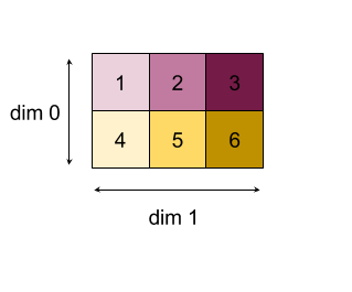
Resultados da redução das dimensões 0 ou 1 com uma função "adicionar":
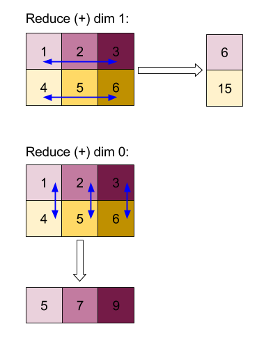
Os dois resultados de redução são matrizes 1D. O diagrama mostra uma como coluna e outra como linha apenas para conveniência visual.
Para um exemplo mais complexo, veja aqui uma matriz 3D. A classificação é 3, a dimensão 0 de tamanho 4, a 1 de tamanho 2 e a 2 de tamanho 3. Para simplificar, os valores de 1 a 6 são replicados na dimensão 0.
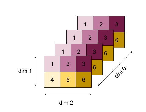
Assim como no exemplo 2D, podemos reduzir apenas uma dimensão. Se reduzirmos a dimensão 0, por exemplo, obtemos uma matriz de classificação 2 em que todos os valores da dimensão 0 foram dobrados em um escalar:
|  4   8  12 |
| 16  20  24 |
Se reduzirmos a dimensão 2, também vamos ter uma matriz de classificação 2 em que todos os valores da dimensão 2 foram dobrados em um escalar:
| 6  15 |
| 6  15 |
| 6  15 |
| 6  15 |
A ordem relativa entre as dimensões restantes na entrada é preservada na saída, mas algumas dimensões podem receber novos números (desde que a classificação mude).
Também podemos reduzir várias dimensões. A adição das dimensões 0 e 1 produz a matriz 1D [20, 28, 36].
Reduzir a matriz 3D em todas as dimensões produz o 84 escalar.
Reduzir variado
Quando N > 1, a aplicação da função de redução é um pouco mais complexa, porque é
aplicada simultaneamente a todas as entradas. Os operandos são fornecidos à
computação na seguinte ordem:
- Valor reduzido em execução para o primeiro operando
- ...
- Valor reduzido em execução para o operando "N"
- Valor de entrada para o primeiro operando
- ...
- Valor de entrada para o operando "N"
Por exemplo, considere a seguinte função de redução, que pode ser usada para calcular o máximo e o argmax de uma matriz 1-D em paralelo:
f: (Float, Int, Float, Int) -> Float, Int
f(max, argmax, value, index):
  if value >= max:
    return (value, index)
  else:
    return (max, argmax)
Para matrizes de entrada 1-D V = Float[N], K = Int[N] e valores init I_V = Float, I_K = Int, o resultado f_(N-1) da redução na única
dimensão de entrada é equivalente ao seguinte aplicativo recursivo:
f_0 = f(I_V, I_K, V_0, K_0)
f_1 = f(f_0.first, f_0.second, V_1, K_1)
...
f_(N-1) = f(f_(N-2).first, f_(N-2).second, V_(N-1), K_(N-1))
Se você aplicar essa redução a uma matriz de valores e a uma matriz de índices sequenciais (ou seja, iota), ela será coiterada nas matrizes e uma tupla contendo o valor máximo e o índice correspondente.
ReducePrecision
Consulte também
XlaBuilder::ReducePrecision.
Modela o efeito da conversão de valores de ponto flutuante em um formato de precisão mais baixa (como IEEE-FP16) e de volta ao formato original. O número de bits de expoente e mantissa no formato de menor precisão pode ser especificado arbitrariamente, embora nem todos os tamanhos de bit possam não ser compatíveis com todas as implementações de hardware.
ReducePrecision(operand, mantissa_bits, exponent_bits)
| Argumentos | Tipo | Semântica |
|---|---|---|
operand |
XlaOp |
matriz do tipo de ponto flutuante T. |
exponent_bits |
int32 |
número de bits expoentes em formato de menor precisão |
mantissa_bits |
int32 |
número de bits de mantissa em formato de menor precisão |
O resultado é uma matriz do tipo T. Os valores de entrada são arredondados para o valor mais próximo
representativo com o número fornecido de bits de mantissa (usando "vinculações a uma semântica"
par). Todos os valores que excedem o intervalo especificado pelo número de bits expoentes são fixados ao infinito positivo ou negativo. Os valores NaN são
mantidos, embora possam ser convertidos em valores NaN canônicos.
O formato de precisão mais baixa precisa ter pelo menos um bit expoente (para distinguir um valor zero de um infinito, já que ambos têm uma mantissa zero) e precisa ter um número não negativo de bits de mantissa. O número de bits de expoente ou
mantissa pode exceder o valor correspondente para o tipo T. A parte correspondente
da conversão é simplesmente um ambiente autônomo.
ReduceScatter
Consulte também
XlaBuilder::ReduceScatter.
reduzem o Scatter é uma operação coletiva que faz um AllReplace efetivamente e
distribui o resultado dividindo-o em blocos shard_count ao longo da
scatter_dimension, e a i da réplica no grupo de réplicas recebe o fragmento
ith.
ReduceScatter(operand, computation, scatter_dim, shard_count,
replica_group_ids, channel_id)
| Argumentos | Tipo | Semântica |
|---|---|---|
operand |
XlaOp |
Matriz ou uma tupla não vazia de matrizes a serem reduzidas entre as réplicas. |
computation |
XlaComputation |
Computação de redução |
scatter_dimension |
int64 |
Dimensão para dispersão. |
shard_count |
int64 |
Número de blocos para dividir scatter_dimension |
replica_groups |
vetor de vetores de int64 |
Grupos entre os quais as reduções são realizadas |
channel_id |
int64 opcional |
ID do canal opcional para comunicação entre módulos |
- Quando
operandé uma tupla de matrizes, a redução de dispersão é realizada em cada elemento da tupla. replica_groupsé uma lista de grupos de réplicas entre os quais a redução é realizada (o ID da réplica atual pode ser recuperado usandoReplicaId). A ordem das réplicas em cada grupo determina a ordem em que o resultado de toda a redução será espalhado.replica_groupsprecisa estar vazio (nesse caso, todas as réplicas pertencem a um único grupo) ou conter o mesmo número de elementos que o número de réplicas. Quando há mais de um grupo de réplicas, todos eles precisam ser do mesmo tamanho. Por exemplo,replica_groups = {0, 2}, {1, 3}executa a redução entre as réplicas0e2, e1e3e, em seguida, distribui o resultado.shard_counté o tamanho de cada grupo de réplicas. Precisamos disso nos casos em quereplica_groupsestá vazio. Sereplica_groupsnão estiver vazio,shard_countprecisará ser igual ao tamanho de cada grupo de réplicas.channel_idé usado para comunicação entre módulos: apenas operaçõesreduce-scattercom o mesmochannel_idpodem se comunicar entre si.
A forma de saída é a forma de entrada com o scatter_dimension reduzido
shard_count vezes menor. Por exemplo, se houver duas réplicas e o
operando tiver os valores [1.0, 2.25] e [3.0, 5.25], respectivamente, nas duas
réplicas, o valor de saída dessa operação em que scatter_dim é 0 será
[4.0] para a primeira réplica e [7.5] para a segunda.
ReduceWindow
Consulte também
XlaBuilder::ReduceWindow.
Aplica uma função de redução a todos os elementos em cada janela de uma sequência de N matrizes multidimensionais, produzindo uma única ou uma tupla de N matrizes multidimensionais como saída. Cada matriz de saída tem o mesmo número de elementos que o
número de posições válidas da janela. Uma camada de pool pode ser expressa como um
ReduceWindow. Assim como no Reduce, o computation aplicado recebe
o init_values no lado esquerdo.
ReduceWindow(operands..., init_values..., computation, window_dimensions,
window_strides, padding)
| Argumentos | Tipo | Semântica |
|---|---|---|
operands |
N XlaOps |
Uma sequência de N matrizes multidimensionais dos tipos T_0,..., T_{N-1}, cada uma representando a área de base em que a janela é colocada. |
init_values |
N XlaOps |
Os valores iniciais N para a redução, um para cada um dos operandos N. Consulte Reduzir para mais detalhes. |
computation |
XlaComputation |
Função de redução do tipo T_0, ..., T_{N-1}, T_0, ..., T_{N-1} -> Collate(T_0, ..., T_{N-1}) para aplicar a elementos em cada janela de todos os operandos de entrada. |
window_dimensions |
ArraySlice<int64> |
matriz de números inteiros para os valores de dimensão da janela |
window_strides |
ArraySlice<int64> |
matriz de números inteiros para valores de passada da janela |
base_dilations |
ArraySlice<int64> |
matriz de números inteiros para valores de dilatação da base |
window_dilations |
ArraySlice<int64> |
matriz de números inteiros para valores de dilatação de janelas |
padding |
Padding |
tipo de padding para a janela (Padding::kSame, que preenche para ter a mesma forma de saída que a entrada se o stride for 1, ou Padding::kValid, que não usa padding e "para" a janela quando ela não cabe mais) |
Em que:
- É necessário que N seja maior ou igual a 1.
- Todas as matrizes de entrada precisam ter as mesmas dimensões.
- Se
N = 1,Collate(T)seráT. - No caso de
N > 1,Collate(T_0, ..., T_{N-1})é uma tupla de elementosNdo tipo(T0,...T{N-1}).
Abaixo do código e da figura, mostramos um exemplo de como usar ReduceWindow. A entrada é uma matriz de tamanho [4x6], e tanto window_dimensions quanto window_stride_dimensions são [2x3].
// Create a computation for the reduction (maximum).
XlaComputation max;
{
  XlaBuilder builder(client_, "max");
  auto y = builder.Parameter(0, ShapeUtil::MakeShape(F32, {}), "y");
  auto x = builder.Parameter(1, ShapeUtil::MakeShape(F32, {}), "x");
  builder.Max(y, x);
  max = builder.Build().value();
}

// Create a ReduceWindow computation with the max reduction computation.
XlaBuilder builder(client_, "reduce_window_2x3");
auto shape = ShapeUtil::MakeShape(F32, {4, 6});
auto input = builder.Parameter(0, shape, "input");
builder.ReduceWindow(
    input,
    /*init_val=*/builder.ConstantLiteral(LiteralUtil::MinValue(F32)),
    *max,
    /*window_dimensions=*/{2, 3},
    /*window_stride_dimensions=*/{2, 3},
    Padding::kValid);
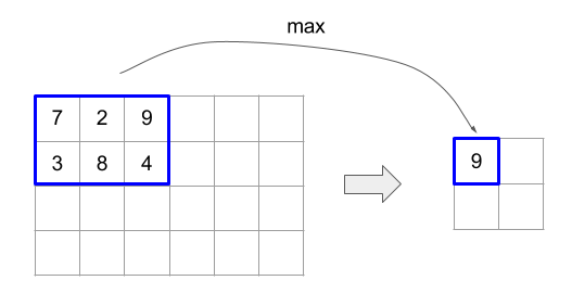
O salto de 1 em uma dimensão especifica que a posição de uma janela na dimensão está a um elemento de distância da janela adjacente. Para especificar que nenhuma janela se sobrepõe, window_stride_dimensions precisa ser igual a window_dimensions. A figura abaixo ilustra o uso de dois valores de stride diferentes. O padding é aplicado a cada dimensão da entrada, e os cálculos são os mesmos, como se a entrada tivesse vindo com as dimensões após o padding.
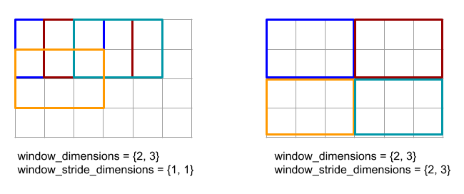
Para um exemplo de padding não trivial, considere calcular o mínimo da janela de redução (o valor inicial é MAX_FLOAT) com a dimensão 3 e o salto 2 na matriz de entrada [10000, 1000, 100, 10, 1]. O preenchimento kValid calcula mínimos em duas janelas válidas: [10000, 1000, 100] e [100, 10, 1], resultando na saída [100, 1]. Primeiro, o padding de kSame preenche a matriz para que a forma após
a janela de redução seja igual à entrada para stride um, adicionando elementos iniciais
em ambos os lados, obtendo [MAX_VALUE, 10000, 1000, 100, 10, 1,
MAX_VALUE]. A execução da janela de redução na matriz preenchida opera em três
janelas [MAX_VALUE, 10000, 1000], [1000, 100, 10], [10, 1, MAX_VALUE] e
gerando [1000, 10, 1].
A ordem de avaliação da função de redução é arbitrária e pode não ser determinista. Portanto, a função de redução não pode ser muito
sensível à reassociação. Consulte a discussão sobre associatividade no
contexto de Reduce para mais detalhes.
ReplicaId
Consulte também
XlaBuilder::ReplicaId.
Retorna o ID exclusivo (escalar U32) da réplica.
ReplicaId()
O ID exclusivo de cada réplica é um número inteiro não assinado no intervalo [0, N),
em que N é o número de réplicas. Como todas as réplicas estão executando o mesmo
programa, uma chamada ReplicaId() no programa retornará um valor diferente em
cada réplica.
Remodelação
Consulte também
XlaBuilder::Reshape
e a operação Collapse.
Remodela as dimensões de uma matriz em uma nova configuração.
Reshape(operand, new_sizes)
Reshape(operand, dimensions, new_sizes)
| Argumentos | Tipo | Semântica |
|---|---|---|
operand |
XlaOp |
matriz do tipo T |
dimensions |
int64 vetor |
ordem em que as dimensões são recolhidas |
new_sizes |
int64 vetor |
vetor de tamanhos de novas dimensões |
Conceitualmente, a reforma primeiro nivela uma matriz em um vetor unidimensional de valores de dados e, em seguida, refina esse vetor em uma nova forma. Os argumentos de entrada
são uma matriz arbitrária do tipo T, um vetor de constante de tempo de compilação de índices de dimensão e um vetor de constante de tempo de compilação de tamanhos de dimensão para o resultado.
Se fornecidos, os valores no vetor dimension precisam ser uma permutação de todas as dimensões de T. Caso contrário, o padrão é {0, ..., rank - 1}. A ordem das
dimensões em dimensions é da dimensão de variação mais lenta (mais importante) para
a de variação mais rápida (mais secundária) no aninhamento de loop, que recolhe a
matriz de entrada em uma única dimensão. O vetor new_sizes determina o tamanho
da matriz de saída. O valor no índice 0 em new_sizes é o tamanho da
dimensão 0, o valor no índice 1 é o tamanho da dimensão 1 e assim por diante. O
produto das dimensões new_size precisa ser igual ao produto dos tamanhos de dimensão
do operando. Ao refinar a matriz recolhida para a matriz multidimensional definida por new_sizes, as dimensões em new_sizes são ordenadas da variação mais baixa (maior) para a mais rápida (menor).
Por exemplo, deixe v ser uma matriz de 24 elementos:
let v = f32[4x2x3] { { {10, 11, 12}, {15, 16, 17} },
                    { {20, 21, 22}, {25, 26, 27} },
                    { {30, 31, 32}, {35, 36, 37} },
                    { {40, 41, 42}, {45, 46, 47} } };

In-order collapse:
let v012_24 = Reshape(v, {0,1,2}, {24});
then v012_24 == f32[24] {10, 11, 12, 15, 16, 17, 20, 21, 22, 25, 26, 27,
                         30, 31, 32, 35, 36, 37, 40, 41, 42, 45, 46, 47};

let v012_83 = Reshape(v, {0,1,2}, {8,3});
then v012_83 == f32[8x3] { {10, 11, 12}, {15, 16, 17},
                          {20, 21, 22}, {25, 26, 27},
                          {30, 31, 32}, {35, 36, 37},
                          {40, 41, 42}, {45, 46, 47} };

Out-of-order collapse:
let v021_24 = Reshape(v, {1,2,0}, {24});
then v012_24 == f32[24]  {10, 20, 30, 40, 11, 21, 31, 41, 12, 22, 32, 42,
                          15, 25, 35, 45, 16, 26, 36, 46, 17, 27, 37, 47};

let v021_83 = Reshape(v, {1,2,0}, {8,3});
then v021_83 == f32[8x3] { {10, 20, 30}, {40, 11, 21},
                          {31, 41, 12}, {22, 32, 42},
                          {15, 25, 35}, {45, 16, 26},
                          {36, 46, 17}, {27, 37, 47} };


let v021_262 = Reshape(v, {1,2,0}, {2,6,2});
then v021_262 == f32[2x6x2] { { {10, 20}, {30, 40},
                              {11, 21}, {31, 41},
                              {12, 22}, {32, 42} },
                             { {15, 25}, {35, 45},
                              {16, 26}, {36, 46},
                              {17, 27}, {37, 47} } };
Como um caso especial, a remodelação pode transformar uma matriz de elemento único em uma escalar e vice-versa. Por exemplo:
Reshape(f32[1x1] { {5} }, {0,1}, {}) == 5;
Reshape(5, {}, {1,1}) == f32[1x1] { {5} };
Rev (reverso)
Consulte também
XlaBuilder::Rev.
Rev(operand, dimensions)
| Argumentos | Tipo | Semântica |
|---|---|---|
operand |
XlaOp |
matriz do tipo T |
dimensions |
ArraySlice<int64> |
dimensões para reverter |
Inverte a ordem dos elementos na matriz operand ao longo do dimensions
especificado, gerando uma matriz de saída da mesma forma. Cada elemento da
matriz do operando em um índice multidimensional é armazenado na matriz de saída em um
índice transformado. O índice multidimensional é transformado pela inversão do índice em cada dimensão a ser invertida (ou seja, se uma dimensão de tamanho N for uma das dimensões reversas, o índice i é transformado em N - 1 - i).
A operação Rev pode ser usada para reverter a matriz de peso de convolução nas duas dimensões de janela durante o cálculo do gradiente em redes neurais.
RngNormal
Consulte também
XlaBuilder::RngNormal.
Constrói uma saída de uma determinada forma com números aleatórios gerados após a \(N(\mu, \sigma)\) distribuição normal. Os parâmetros \(\mu\) e \(\sigma\)e a forma de saída precisam ter um tipo elementar de ponto flutuante. Além disso, os parâmetros precisam ter valor escalar.
RngNormal(mu, sigma, shape)
| Argumentos | Tipo | Semântica |
|---|---|---|
mu |
XlaOp |
Escalar do tipo T especificando a média dos números gerados |
sigma |
XlaOp |
Escalar do tipo T especificando o desvio padrão do tipo |
shape |
Shape |
Forma de saída do tipo T |
RngUniform
Consulte também
XlaBuilder::RngUniform.
Constrói uma saída de uma determinada forma com números aleatórios gerados seguindo a distribuição uniforme durante o intervalo \([a,b)\). Os parâmetros e o tipo de elemento de saída precisam ser um tipo booleano, um tipo integral ou um tipo de ponto flutuante, e os tipos precisam ser consistentes. Atualmente, os back-ends de CPU e GPU oferecem suporte apenas a F64, F32, F16, BF16, S64, U64, S32 e U32. Além disso, os parâmetros precisam ter valor escalar. Se \(b <= a\) , o resultado for definido pela implementação.
RngUniform(a, b, shape)
| Argumentos | Tipo | Semântica |
|---|---|---|
a |
XlaOp |
Escalar do tipo T especificando o limite mínimo do intervalo |
b |
XlaOp |
Escalar do tipo T especificando o limite máximo do intervalo |
shape |
Shape |
Forma de saída do tipo T |
RngBitGenerator
Gera uma saída com uma determinada forma preenchida com bits aleatórios uniformes usando o algoritmo especificado (ou padrão de back-end) e retorna um estado atualizado (com a mesma forma do estado inicial) e os dados aleatórios gerados.
O estado inicial é a situação inicial da geração atual do número aleatório. Isso e o formato necessário e os valores válidos dependem do algoritmo usado.
A saída certamente será uma função determinística do estado inicial, mas não há garantia de que ela seja determinista entre back-ends e diferentes versões do compilador.
RngBitGenerator(algorithm, key, shape)
| Argumentos | Tipo | Semântica |
|---|---|---|
algorithm |
RandomAlgorithm |
Algoritmo PRNG a ser usado. |
initial_state |
XlaOp |
Estado inicial do algoritmo PRNG. |
shape |
Shape |
Forma de saída dos dados gerados. |
Valores disponíveis para algorithm:
rng_default: algoritmo específico de back-end com requisitos de forma específicos do back-end.rng_three_fry: algoritmo PRNG baseado em contador do ThreeFry. A formainitial_stateéu64[2]com valores arbitrários. Salmon e outros, SC 2011. Números aleatórios paralelos: 1, 2, 3.rng_philox: algoritmo Philox para gerar números aleatórios em paralelo. O formatoinitial_stateéu64[3]com valores arbitrários. Salmon e outros, SC 2011. Números aleatórios paralelos: 1, 2, 3.
Dispersão
A operação de dispersão do XLA gera uma sequência de resultados, que são os valores
da matriz de entrada operands, com várias frações (em índices especificados por
scatter_indices) atualizadas com a sequência de valores em updates usando
update_computation.
Consulte também
XlaBuilder::Scatter.
scatter(operands..., scatter_indices, updates..., update_computation,
index_vector_dim, update_window_dims, inserted_window_dims,
scatter_dims_to_operand_dims)
| Argumentos | Tipo | Semântica |
|---|---|---|
operands |
Sequência de N XlaOp |
N matrizes dos tipos T_0, ..., T_N em que serão espalhadas. |
scatter_indices |
XlaOp |
Matriz contendo os índices iniciais das fatias que devem ser distribuídas. |
updates |
Sequência de N XlaOp |
N matrizes dos tipos T_0, ..., T_N. updates[i] contém os valores que precisam ser usados para espalhar operands[i]. |
update_computation |
XlaComputation |
Computação a ser usada para combinar os valores existentes na matriz de entrada e as atualizações durante a dispersão. Esse cálculo precisa ser do tipo T_0, ..., T_N, T_0, ..., T_N -> Collate(T_0, ..., T_N). |
index_vector_dim |
int64 |
A dimensão em scatter_indices que contém os índices iniciais. |
update_window_dims |
ArraySlice<int64> |
O conjunto de dimensões no formato updates que são dimensões de janela. |
inserted_window_dims |
ArraySlice<int64> |
O conjunto de dimensões de janela que precisam ser inseridas na forma updates. |
scatter_dims_to_operand_dims |
ArraySlice<int64> |
Uma dimensão é mapeada dos índices de dispersão para o espaço de índice do operando. Essa matriz é interpretada como um mapeamento de i para scatter_dims_to_operand_dims[i] . Precisa ser individual e total. |
indices_are_sorted |
bool |
Indica se os índices serão classificados pelo autor da chamada. |
Em que:
- É necessário que N seja maior ou igual a 1.
operands[0], ... eoperands[N-1] precisam ter as mesmas dimensões.updates[0], ... eupdates[N-1] precisam ter as mesmas dimensões.- Se
N = 1,Collate(T)seráT. - No caso de
N > 1,Collate(T_0, ..., T_N)é uma tupla de elementosNdo tipoT.
Se index_vector_dim for igual a scatter_indices.rank, vamos considerar implicitamente
scatter_indices como uma dimensão 1 à direita.
Definimos update_scatter_dims do tipo ArraySlice<int64> como o conjunto de
dimensões na forma updates que não estão em update_window_dims, em ordem
crescente.
Os argumentos de dispersão precisam seguir estas restrições:
Cada matriz de
updatesprecisa ser da classificaçãoupdate_window_dims.size + scatter_indices.rank - 1.Os limites da dimensão
iem cada matrizupdatesprecisam estar em conformidade com o seguinte:- Se
iestiver presente emupdate_window_dims(ou seja, igual aupdate_window_dims[k] para algunsk), o limite da dimensãoiemupdatesnão poderá exceder o limite correspondente deoperandapós considerarinserted_window_dims(ou seja,adjusted_window_bounds[k], em queadjusted_window_boundscontém os limites deoperandcom os limites nos índicesinserted_window_dimsremovidos). - Se
iestiver presente emupdate_scatter_dims(ou seja, igual aupdate_scatter_dims[k] para algunsk), o limite da dimensãoiemupdatesprecisará ser igual ao limite correspondente descatter_indices, ignorandoindex_vector_dim(ou seja,scatter_indices.shape.dims[k], sekfor <index_vector_dimescatter_indices.shape.dims[k+1]).
- Se
update_window_dimsprecisa estar em ordem crescente, não ter números de dimensão repetidos e estar no intervalo[0, updates.rank).inserted_window_dimsprecisa estar em ordem crescente, não ter números de dimensão repetidos e estar no intervalo[0, operand.rank).operand.rankprecisa ser igual à soma deupdate_window_dims.sizeeinserted_window_dims.size.scatter_dims_to_operand_dims.sizeprecisa ser igual ascatter_indices.shape.dims[index_vector_dim] e os valores precisam estar no intervalo[0, operand.rank).
Para um determinado índice U em cada matriz updates, o índice correspondente I na matriz operands correspondente em que essa atualização precisa ser aplicada é calculado da seguinte maneira:
- Permita que
G= {U[k] parakemupdate_scatter_dims}. UseGpara procurar um vetor de índiceSna matrizscatter_indicesde modo queS[i] =scatter_indices[Combine(G,i)] em que Combine(A, b) insira b em posiçõesindex_vector_dimem A. - Crie um índice
SinemoperandusandoSespalhandoScom o mapascatter_dims_to_operand_dims. Mais formalmente:Sin[scatter_dims_to_operand_dims[k]] =S[k] sek<scatter_dims_to_operand_dims.size.Sin[_] =0.
- Crie um índice
Winem cada matrizoperandsespalhando os índices emupdate_window_dimsemUde acordo cominserted_window_dims. Mais formalmente:Win[window_dims_to_operand_dims(k)] =U[k] sekestiver emupdate_window_dims, em quewindow_dims_to_operand_dimsé a função monotônica com o domínio [0,update_window_dims.size) e o intervalo [0,operand.rank) \inserted_window_dims. Por exemplo, seupdate_window_dims.sizefor4,operand.rankfor6einserted_window_dimsfor {0,2}, entãowindow_dims_to_operand_dimsserá {0→1,1→3,2→4,3→5}).Win[_] =0.
IéWin+Sin, em que + é uma adição de elemento.
Em resumo, é possível definir a operação de dispersão da seguinte maneira.
- Inicialize
outputcomoperands, ou seja, para todos os índicesJ, para todos os índicesOna matrizoperands[J]:
output[J][O] =operands[J][O] - Para cada índice
Una matrizupdates[J] e o índice correspondenteOna matrizoperand[J], seOfor um índice válido paraoutput:
(output[0][O], ...,output[N-1][O]) =update_computation(output[0][O], ..., ,output[N-1][O],updates[0][U], ...,updates[N-1][U])
A ordem em que as atualizações são aplicadas não é determinista. Portanto, quando vários
índices em updates se referem ao mesmo índice em operands, o valor
correspondente em output será não determinístico.
O primeiro parâmetro transmitido para a update_computation será sempre o valor atual da matriz output, e o segundo parâmetro sempre será o valor da matriz updates. Isso é importante
especificamente nos casos em que update_computation não é comutativo.
Se indices_are_sorted for definido como verdadeiro, o XLA poderá presumir que start_indices
são classificados (em ordem crescente de start_index_map) pelo usuário. Se não forem, a semântica será implementada.
informalmente, a op de dispersão pode ser vista como um inverso da operação de coleta, ou seja, a op de dispersão atualiza os elementos na entrada que são extraídos pela operação de coleta correspondente.
Para uma descrição informal detalhada e exemplos, consulte a seção "Descrição informacional" em Gather.
Selecione
Consulte também
XlaBuilder::Select.
Constrói uma matriz de saída a partir de elementos de duas matrizes de entrada, com base nos valores de uma matriz de predicado.
Select(pred, on_true, on_false)
| Argumentos | Tipo | Semântica |
|---|---|---|
pred |
XlaOp |
matriz do tipo PRED |
on_true |
XlaOp |
matriz do tipo T |
on_false |
XlaOp |
matriz do tipo T |
As matrizes on_true e on_false precisam ter a mesma forma. Essa também é a forma da matriz de saída. A matriz pred precisa ter a mesma dimensionalidade que on_true e on_false, com o tipo de elemento PRED.
Para cada elemento P de pred, o elemento correspondente da matriz de saída será
extraído de on_true se o valor de P for true e de on_false se o
valor de P for false. Como uma forma restrita de transmissão,
pred pode ser um escalar do tipo PRED. Nesse caso, a matriz de saída será extraída
totalmente de on_true se pred for true e de on_false se pred for false.
Exemplo com pred não escalar:
let pred: PRED[4] = {true, false, false, true};
let v1: s32[4] = {1, 2, 3, 4};
let v2: s32[4] = {100, 200, 300, 400};
==>
Select(pred, v1, v2) = s32[4]{1, 200, 300, 4};
Exemplo com pred escalar:
let pred: PRED = true;
let v1: s32[4] = {1, 2, 3, 4};
let v2: s32[4] = {100, 200, 300, 400};
==>
Select(pred, v1, v2) = s32[4]{1, 2, 3, 4};
Há suporte para seleções entre tuplas. As tuplas são consideradas tipos escalares
para essa finalidade. Se on_true e on_false forem tuplas (que precisam ter a mesma forma), pred precisa ser um escalar do tipo PRED.
SelectAndScatter
Consulte também
XlaBuilder::SelectAndScatter.
Essa operação pode ser considerada como uma operação composta que primeiro calcula
ReduceWindow na matriz operand para selecionar um elemento de cada janela e,
em seguida, espalha a matriz source para os índices dos elementos selecionados para
construir uma matriz de saída com a mesma forma da matriz de operandos. A função binária select é usada para selecionar um elemento de cada janela aplicando-o em cada janela e é chamada com a propriedade de que o vetor de índice do primeiro parâmetro é lexicograficamente menor que o vetor de índice do segundo parâmetro. A função select retornará true se o primeiro parâmetro for
selecionado e retornará false se o segundo for selecionado. A
função precisar manter a transitividade (ou seja, se select(a, b) e select(b, c) forem
true, select(a, c) também será true) para que o elemento selecionado
não dependa da ordem dos elementos transferidos em uma determinada janela.
A função scatter é aplicada a cada índice selecionado na matriz de saída. Ela usa dois parâmetros escalares:
- Valor atual no índice selecionado na matriz de saída
- O valor de dispersão de
sourceque se aplica ao índice selecionado
Ela combina os dois parâmetros e retorna um valor escalar usado para atualizar
o valor no índice selecionado na matriz de saída. Inicialmente, todos os índices da
matriz de saída são definidos como init_value.
A matriz de saída tem a mesma forma que a matriz operand, e a matriz source
precisa ter a mesma forma do resultado da aplicação de uma operação ReduceWindow
na matriz operand. SelectAndScatter pode ser usado para retropropagar os valores do gradiente para uma camada de pooling em uma rede neural.
SelectAndScatter(operand, select, window_dimensions, window_strides,
padding, source, init_value, scatter)
| Argumentos | Tipo | Semântica |
|---|---|---|
operand |
XlaOp |
matriz do tipo T sobre a qual as janelas deslizam |
select |
XlaComputation |
Computação binária do tipo T, T -> PRED para aplicar a todos os elementos em cada janela. Retorna true se o primeiro parâmetro for selecionado e false se o segundo parâmetro for selecionado. |
window_dimensions |
ArraySlice<int64> |
matriz de números inteiros para os valores de dimensão da janela |
window_strides |
ArraySlice<int64> |
matriz de números inteiros para valores de passada da janela |
padding |
Padding |
tipo de padding da janela (Padding::kSame ou Padding::kValid) |
source |
XlaOp |
matriz do tipo T com os valores a serem espalhados |
init_value |
XlaOp |
valor escalar do tipo T para o valor inicial da matriz de saída |
scatter |
XlaComputation |
Computação binária do tipo T, T -> T para aplicar cada elemento de origem de dispersão ao elemento de destino |
A figura abaixo mostra exemplos de uso de SelectAndScatter, com a função select
calculando o valor máximo entre os parâmetros. Observe que, quando as
janelas se sobrepõem, como na figura (2) abaixo, um índice da matriz operand pode
ser selecionado várias vezes por janelas diferentes. Na figura, o elemento do
valor 9 é selecionado pelas duas janelas superiores (azul e vermelho), e a função de adição binária scatter produz o elemento de saída do valor 8 (2 + 6).
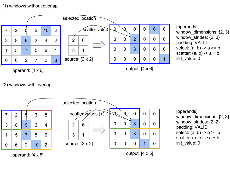
A ordem de avaliação da função scatter é arbitrária e pode não ser determinista. Portanto, a função scatter não pode ser muito
sensível à reassociação. Consulte a discussão sobre associatividade no
contexto de Reduce para mais detalhes.
Enviar
Consulte também
XlaBuilder::Send.
Send(operand, channel_handle)
| Argumentos | Tipo | Semântica |
|---|---|---|
operand |
XlaOp |
dados a serem enviados (matriz do tipo T) |
channel_handle |
ChannelHandle |
identificador exclusivo para cada par de envio/recv |
Envia os dados de operando fornecidos para uma instrução Recv em outro cálculo
que compartilha o mesmo identificador de canal. Não retorna nenhum dado.
Semelhante à operação Recv, a API do cliente da operação Send representa
a comunicação síncrona e é decomposta internamente em duas instruções HLO
(Send e SendDone) para ativar as transferências de dados assíncronas. Consulte também
HloInstruction::CreateSend e HloInstruction::CreateSendDone.
Send(HloInstruction operand, int64 channel_id)
Inicia uma transferência assíncrona do operando para os recursos alocados pela
instrução Recv com o mesmo ID do canal. Retorna um contexto, que é
usado por uma instrução SendDone a seguir para aguardar a conclusão da
transferência de dados. O contexto é uma tupla de {Operand (shape), request identificador
(U32)} e só pode ser usada por uma instrução SendDone.
SendDone(HloInstruction context)
Em um contexto criado por uma instrução Send, ele aguarda a conclusão da transferência de dados. A instrução não retorna nenhum dado.
Programação de instruções do canal
A ordem de execução das quatro instruções para cada canal (Recv, RecvDone, Send, SendDone) é mostrada abaixo.
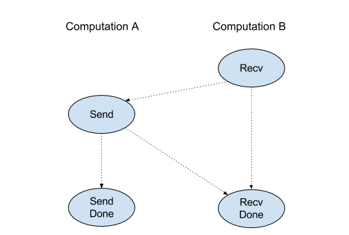
Recvacontece antes deSendSendacontece antes deRecvDoneRecvacontece antes deRecvDoneSendacontece antes deSendDone
Quando os compiladores de back-end geram uma programação linear para cada computação que se comunica por meio de instruções de canal, não pode haver ciclos entre os cálculos. Por exemplo, as programações abaixo levam a impasses.
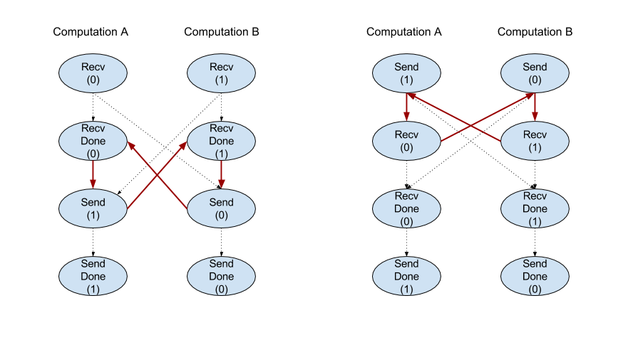
Fração
Consulte também
XlaBuilder::Slice.
O fracionamento extrai uma submatriz da matriz de entrada. A submatriz é da mesma classificação que a entrada e contém os valores dentro de uma caixa delimitadora dentro da matriz de entrada, em que as dimensões e os índices da caixa delimitadora são fornecidos como argumentos para a operação de fração.
Slice(operand, start_indices, limit_indices, strides)
| Argumentos | Tipo | Semântica |
|---|---|---|
operand |
XlaOp |
Matriz dimensional N do tipo T |
start_indices |
ArraySlice<int64> |
Lista de N números inteiros com os índices iniciais da fatia de cada dimensão. Os valores precisam ser maiores ou iguais a zero. |
limit_indices |
ArraySlice<int64> |
Lista de N números inteiros com os índices finais (exclusivos) para a fatia de cada dimensão. Cada valor precisa ser maior ou igual ao respectivo valor de start_indices para a dimensão e menor ou igual ao tamanho da dimensão. |
strides |
ArraySlice<int64> |
Lista de N números inteiros que decide o stride de entrada da fração. A fatia escolhe cada elemento strides[d] na dimensão d. |
Exemplo unidimensional:
let a = {0.0, 1.0, 2.0, 3.0, 4.0}
Slice(a, {2}, {4}) produces:
  {2.0, 3.0}
Exemplo de bidimensional:
let b =
 { {0.0,  1.0,  2.0},
   {3.0,  4.0,  5.0},
   {6.0,  7.0,  8.0},
   {9.0, 10.0, 11.0} }

Slice(b, {2, 1}, {4, 3}) produces:
  { { 7.0,  8.0},
    {10.0, 11.0} }
Classificar
Consulte também
XlaBuilder::Sort.
Sort(operands, comparator, dimension, is_stable)
| Argumentos | Tipo | Semântica |
|---|---|---|
operands |
ArraySlice<XlaOp> |
Os operandos a serem classificados. |
comparator |
XlaComputation |
O cálculo do comparador a ser usado. |
dimension |
int64 |
A dimensão pela qual classificar. |
is_stable |
bool |
Define se a classificação estável precisa ser usada. |
Se apenas um operando for fornecido:
Se o operando for um tensor de classificação-1 (uma matriz), o resultado será uma matriz classificada. Se você quiser classificar a matriz em ordem crescente, o comparador precisará realizar uma comparação de menor que. Formalmente, depois que a matriz é classificada, ela é mantida para todas as posições de índice
i, jcomi < jquecomparator(value[i], value[j]) = comparator(value[j], value[i]) = falseoucomparator(value[i], value[j]) = true.Se o operando tiver uma classificação mais alta, ele será classificado de acordo com a dimensão fornecida. Por exemplo, para um tensor de classificação 2 (uma matriz), um valor de dimensão de
0classificará cada coluna independentemente, e um valor de dimensão de1classificará cada linha de maneira independente. Se nenhum número de dimensão for fornecido, a última dimensão será escolhida por padrão. Para a dimensão que é classificada, a mesma ordem de classificação é aplicada no caso de classificação 1.
Se os operandos n > 1 forem fornecidos:
Todos os operandos
nprecisam ser tensores com as mesmas dimensões. Os tipos de elemento dos tensores podem ser diferentes.Todos os operandos são classificados juntos, não individualmente. Conceitualmente, os operandos são tratados como uma tupla. Ao verificar se os elementos de cada operando nas posições de índice
iejprecisam ser trocados, o comparador é chamado com parâmetros escalares2 * n, em que o parâmetro2 * kcorresponde ao valor na posiçãoido operandok-th, e o parâmetro2 * k + 1corresponde ao valor na posiçãojdo operandok-th. Normalmente, o comparador compara os parâmetros2 * ke2 * k + 1entre si e possivelmente usa outros pares de parâmetros como desempatadores.O resultado é uma tupla que consiste nos operandos em ordem classificada (junto à dimensão fornecida, como acima). O operando
i-thda tupla corresponde ao operandoi-thde Sort.
Por exemplo, se houver três operandos operand0 = [3, 1],
operand1 = [42, 50] e operand2 = [-3.0, 1.1], e o comparador comparar
apenas os valores de operand0 com "menor que", a saída da classificação será a
tupla ([1, 3], [50, 42], [1.1, -3.0]).
Se is_stable for definido como verdadeiro, a classificação será estável, ou seja, se
houver elementos considerados iguais pelo comparador, a
ordem relativa dos valores iguais será preservada. Dois elementos, e1 e e2, serão
iguais se, e somente se, comparator(e1, e2) = comparator(e2, e1) = false. Por
padrão, is_stable é definido como falso.
Transposição
Consulte também a operação tf.reshape.
Transpose(operand)
| Argumentos | Tipo | Semântica |
|---|---|---|
operand |
XlaOp |
O operando a ser transposto. |
permutation |
ArraySlice<int64> |
Como permutar as dimensões. |
Permuta as dimensões do operando com a permutação fornecida. Portanto, ∀ i . 0 ≤ i < rank ⇒ input_dimensions[permutation[i]] = output_dimensions[i].
É o mesmo que Reshape(opera, permutação, Permute(permutação, opera.shape.dimensions)).
TriangularSolve
Consulte também
XlaBuilder::TriangularSolve.
Resolve sistemas de equações lineares com matrizes de coeficientes triangulares
superiores ou menores por substituição para frente ou para trás. Transmitindo pelas dimensões
principais, essa rotina resolve um dos sistemas de matriz op(a) * x =
b, ou x * op(a) = b, para a variável x, com base em a e b, em que op(a) é
op(a) = a, op(a) = Transpose(a) ou op(a) = Conj(Transpose(a)).
TriangularSolve(a, b, left_side, lower, unit_diagonal, transpose_a)
| Argumentos | Tipo | Semântica |
|---|---|---|
a |
XlaOp |
uma matriz de classificação > 2 de um tipo complexo ou de ponto flutuante com a forma [..., M, M]; |
b |
XlaOp |
Uma matriz de classificação > 2 do mesmo tipo com a forma [..., M, K] se left_side for verdadeiro. Caso contrário, [..., K, M]. |
left_side |
bool |
indica se é necessário resolver um sistema no formato op(a) * x = b (true) ou x * op(a) = b (false). |
lower |
bool |
se o triângulo superior ou inferior de a será usado. |
unit_diagonal |
bool |
Se true, os elementos diagonais de a serão considerados 1 e não serão acessados. |
transpose_a |
Transpose |
usar a como está, transpor ou usar a transposição conjugada dela. |
Os dados de entrada são lidos apenas do triângulo inferior/superior de a, dependendo do
valor de lower. Os valores do outro triângulo são ignorados. Os dados de saída são
retornados no mesmo triângulo. Os valores no outro triângulo são
definidos pela implementação e podem ser qualquer coisa.
Se a classificação de a e b for maior que 2, elas serão tratadas como lotes de matrizes, em que todas, exceto as dimensões 2 secundárias, são dimensões de lote. a e b precisam ter dimensões de lote iguais.
Tupla
Consulte também
XlaBuilder::Tuple.
Uma tupla contendo um número variável de identificadores de dados, cada um com um formato próprio.
Isso é análogo a std::tuple em C++. Conceitualmente:
let v: f32[10] = f32[10]{0, 1, 2, 3, 4, 5, 6, 7, 8, 9};
let s: s32 = 5;
let t: (f32[10], s32) = tuple(v, s);
As tuplas podem ser desconstruídas (acessadas) pela operação GetTupleElement.
Embora
Consulte também
XlaBuilder::While.
While(condition, body, init)
| Argumentos | Tipo | Semântica |
|---|---|---|
condition |
XlaComputation |
XlaComputation do tipo T -> PRED, que define a condição de encerramento do loop. |
body |
XlaComputation |
XlaComputation do tipo T -> T, que define o corpo da repetição. |
init |
T |
Valor inicial do parâmetro de condition e body. |
Executa o body sequencialmente até que o condition falhe. Isso é semelhante a
um loop "while" comum em muitos outros idiomas, exceto pelas diferenças e
restrições listadas abaixo.
- Um nó
Whileretorna um valor do tipoT, que é o resultado da última execução dobody. - A forma do tipo
Té determinada estaticamente e precisa ser a mesma em todas as iterações.
Os parâmetros T dos cálculos são inicializados com o valor init na primeira iteração e atualizados automaticamente para o novo resultado de body em cada iteração subsequente.
Um caso de uso principal do nó While é implementar a execução repetida de treinamento em redes neurais. Veja abaixo um pseudocódigo simplificado com um gráfico que representa a computação. O código pode ser encontrado em
while_test.cc.
O tipo T neste exemplo é um Tuple que consiste em um int32 para a
contagem de iterações e um vector[10] para o acumulador. Por 1.000 iterações, o
loop continua adicionando um vetor constante ao acumulador.
// Pseudocode for the computation.
init = {0, zero_vector[10]} // Tuple of int32 and float[10].
result = init;
while (result(0) < 1000) {
  iteration = result(0) + 1;
  new_vector = result(1) + constant_vector[10];
  result = {iteration, new_vector};
}