
| | |  Ver fuente en GitHub Ver fuente en GitHub | |
Este tutorial clasificación de texto entrena una red neuronal recurrente en la IMDB gran película de opinión conjunto de datos para el análisis de los sentimientos.
Configuración
import numpy as np

import tensorflow_datasets as tfds
import tensorflow as tf

tfds.disable_progress_bar()
Importación matplotlib y crear una función de ayuda a los gráficos de la trama:
import matplotlib.pyplot as plt


def plot_graphs(history, metric):
  plt.plot(history.history[metric])
  plt.plot(history.history['val_'+metric], '')
  plt.xlabel("Epochs")
  plt.ylabel(metric)
  plt.legend([metric, 'val_'+metric])
Configurar canalización de entrada
El IMDB amplia reseña de la película conjunto de datos es un conjunto de datos binarios de clasificación-todas las opiniones tienen ya sea positiva o sentimiento negativo.
Descargar el conjunto de datos utilizando TFDS . Ver el tutorial de texto de carga para obtener más información sobre cómo cargar este tipo de datos de forma manual.
dataset, info = tfds.load('imdb_reviews', with_info=True,
                          as_supervised=True)
train_dataset, test_dataset = dataset['train'], dataset['test']

train_dataset.element_spec
(TensorSpec(shape=(), dtype=tf.string, name=None),
 TensorSpec(shape=(), dtype=tf.int64, name=None))
Inicialmente, esto devuelve un conjunto de datos de (texto, pares de etiquetas):
for example, label in train_dataset.take(1):
  print('text: ', example.numpy())
  print('label: ', label.numpy())
text:  b"This was an absolutely terrible movie. Don't be lured in by Christopher Walken or Michael Ironside. Both are great actors, but this must simply be their worst role in history. Even their great acting could not redeem this movie's ridiculous storyline. This movie is an early nineties US propaganda piece. The most pathetic scenes were those when the Columbian rebels were making their cases for revolutions. Maria Conchita Alonso appeared phony, and her pseudo-love affair with Walken was nothing but a pathetic emotional plug in a movie that was devoid of any real meaning. I am disappointed that there are movies like this, ruining actor's like Christopher Walken's good name. I could barely sit through it."
label:  0
A continuación mezclar los datos de formación y crear lotes de estos (text, label) pares:
BUFFER_SIZE = 10000
BATCH_SIZE = 64
train_dataset = train_dataset.shuffle(BUFFER_SIZE).batch(BATCH_SIZE).prefetch(tf.data.AUTOTUNE)
test_dataset = test_dataset.batch(BATCH_SIZE).prefetch(tf.data.AUTOTUNE)
for example, label in train_dataset.take(1):
  print('texts: ', example.numpy()[:3])
  print()
  print('labels: ', label.numpy()[:3])
texts:  [b'This is arguably the worst film I have ever seen, and I have quite an appetite for awful (and good) movies. It could (just) have managed a kind of adolescent humour if it had been consistently tongue-in-cheek --\xc3\xa0 la ROCKY HORROR PICTURE SHOW, which was really very funny. Other movies, like PLAN NINE FROM OUTER SPACE, manage to be funny while (apparently) trying to be serious. As to the acting, it looks like they rounded up brain-dead teenagers and asked them to ad-lib the whole production. Compared to them, Tom Cruise looks like Alec Guinness. There was one decent interpretation -- that of the older ghoul-busting broad on the motorcycle.'
 b"I saw this film in the worst possible circumstance. I'd already missed 15 minutes when I woke up to it on an international flight between Sydney and Seoul. I didn't know what I was watching, I thought maybe it was a movie of the week, but quickly became riveted by the performance of the lead actress playing a young woman who's child had been kidnapped. The premise started taking twist and turns I didn't see coming and by the end credits I was scrambling through the the in-flight guide to figure out what I had just watched. Turns out I was belatedly discovering Do-yeon Jeon who'd won Best Actress at Cannes for the role. I don't know if Secret Sunshine is typical of Korean cinema but I'm off to the DVD store to discover more."
 b"Hello. I am Paul Raddick, a.k.a. Panic Attack of WTAF, Channel 29 in Philadelphia. Let me tell you about this god awful movie that powered on Adam Sandler's film career but was digitized after a short time.<br /><br />Going Overboard is about an aspiring comedian played by Sandler who gets a job on a cruise ship and fails...or so I thought. Sandler encounters babes that like History of the World Part 1 and Rebound. The babes were supposed to be engaged, but, actually, they get executed by Sawtooth, the meanest cannibal the world has ever known. Adam Sandler fared bad in Going Overboard, but fared better in Big Daddy, Billy Madison, and Jen Leone's favorite, 50 First Dates. Man, Drew Barrymore was one hot chick. Spanglish is red hot, Going Overboard ain't Dooley squat! End of file."]

labels:  [0 1 0]
Crea el codificador de texto
El texto en bruto cargado por tfds necesita ser procesada antes de que pueda ser utilizado en un modelo. La forma más sencilla de texto proceso de formación está utilizando el TextVectorization capa. Esta capa tiene muchas capacidades, pero este tutorial se adhiere al comportamiento predeterminado.
Crear la capa, y aprobar el texto del conjunto de datos a la capa de .adapt método:
VOCAB_SIZE = 1000
encoder = tf.keras.layers.TextVectorization(
    max_tokens=VOCAB_SIZE)
encoder.adapt(train_dataset.map(lambda text, label: text))
El .adapt método establece el vocabulario de la capa. Aquí están las primeras 20 fichas. Después del relleno y los tokens desconocidos, se ordenan por frecuencia:
vocab = np.array(encoder.get_vocabulary())
vocab[:20]
array(['', '[UNK]', 'the', 'and', 'a', 'of', 'to', 'is', 'in', 'it', 'i',
       'this', 'that', 'br', 'was', 'as', 'for', 'with', 'movie', 'but'],
      dtype='<U14')
Una vez que se establece el vocabulario, la capa puede codificar texto en índices. Los tensores de índices se 0-acolchado en la secuencia más larga en el lote (a menos que establezca un fijo output_sequence_length ):
encoded_example = encoder(example)[:3].numpy()
encoded_example
array([[ 11,   7,   1, ...,   0,   0,   0],
       [ 10, 208,  11, ...,   0,   0,   0],
       [  1,  10, 237, ...,   0,   0,   0]])
Con la configuración predeterminada, el proceso no es completamente reversible. Hay tres razones principales para ello:
- El valor por defecto para
preprocessing.TextVectorization'sstandardizeargumento es"lower_and_strip_punctuation". - El tamaño limitado del vocabulario y la falta de respaldo basado en caracteres dan como resultado algunos tokens desconocidos.
for n in range(3):
  print("Original: ", example[n].numpy())
  print("Round-trip: ", " ".join(vocab[encoded_example[n]]))
  print()
Original:  b'This is arguably the worst film I have ever seen, and I have quite an appetite for awful (and good) movies. It could (just) have managed a kind of adolescent humour if it had been consistently tongue-in-cheek --\xc3\xa0 la ROCKY HORROR PICTURE SHOW, which was really very funny. Other movies, like PLAN NINE FROM OUTER SPACE, manage to be funny while (apparently) trying to be serious. As to the acting, it looks like they rounded up brain-dead teenagers and asked them to ad-lib the whole production. Compared to them, Tom Cruise looks like Alec Guinness. There was one decent interpretation -- that of the older ghoul-busting broad on the motorcycle.'
Round-trip:  this is [UNK] the worst film i have ever seen and i have quite an [UNK] for awful and good movies it could just have [UNK] a kind of [UNK] [UNK] if it had been [UNK] [UNK] [UNK] la [UNK] horror picture show which was really very funny other movies like [UNK] [UNK] from [UNK] space [UNK] to be funny while apparently trying to be serious as to the acting it looks like they [UNK] up [UNK] [UNK] and [UNK] them to [UNK] the whole production [UNK] to them tom [UNK] looks like [UNK] [UNK] there was one decent [UNK] that of the older [UNK] [UNK] on the [UNK]

Original:  b"I saw this film in the worst possible circumstance. I'd already missed 15 minutes when I woke up to it on an international flight between Sydney and Seoul. I didn't know what I was watching, I thought maybe it was a movie of the week, but quickly became riveted by the performance of the lead actress playing a young woman who's child had been kidnapped. The premise started taking twist and turns I didn't see coming and by the end credits I was scrambling through the the in-flight guide to figure out what I had just watched. Turns out I was belatedly discovering Do-yeon Jeon who'd won Best Actress at Cannes for the role. I don't know if Secret Sunshine is typical of Korean cinema but I'm off to the DVD store to discover more."
Round-trip:  i saw this film in the worst possible [UNK] id already [UNK] [UNK] minutes when i [UNK] up to it on an [UNK] [UNK] between [UNK] and [UNK] i didnt know what i was watching i thought maybe it was a movie of the [UNK] but quickly became [UNK] by the performance of the lead actress playing a young woman whos child had been [UNK] the premise started taking twist and turns i didnt see coming and by the end credits i was [UNK] through the the [UNK] [UNK] to figure out what i had just watched turns out i was [UNK] [UNK] [UNK] [UNK] [UNK] [UNK] best actress at [UNK] for the role i dont know if secret [UNK] is typical of [UNK] cinema but im off to the dvd [UNK] to [UNK] more

Original:  b"Hello. I am Paul Raddick, a.k.a. Panic Attack of WTAF, Channel 29 in Philadelphia. Let me tell you about this god awful movie that powered on Adam Sandler's film career but was digitized after a short time.<br /><br />Going Overboard is about an aspiring comedian played by Sandler who gets a job on a cruise ship and fails...or so I thought. Sandler encounters babes that like History of the World Part 1 and Rebound. The babes were supposed to be engaged, but, actually, they get executed by Sawtooth, the meanest cannibal the world has ever known. Adam Sandler fared bad in Going Overboard, but fared better in Big Daddy, Billy Madison, and Jen Leone's favorite, 50 First Dates. Man, Drew Barrymore was one hot chick. Spanglish is red hot, Going Overboard ain't Dooley squat! End of file."
Round-trip:  [UNK] i am paul [UNK] [UNK] [UNK] [UNK] of [UNK] [UNK] [UNK] in [UNK] let me tell you about this god awful movie that [UNK] on [UNK] [UNK] film career but was [UNK] after a short [UNK] br going [UNK] is about an [UNK] [UNK] played by [UNK] who gets a job on a [UNK] [UNK] and [UNK] so i thought [UNK] [UNK] [UNK] that like history of the world part 1 and [UNK] the [UNK] were supposed to be [UNK] but actually they get [UNK] by [UNK] the [UNK] [UNK] the world has ever known [UNK] [UNK] [UNK] bad in going [UNK] but [UNK] better in big [UNK] [UNK] [UNK] and [UNK] [UNK] favorite [UNK] first [UNK] man [UNK] [UNK] was one hot [UNK] [UNK] is red hot going [UNK] [UNK] [UNK] [UNK] end of [UNK]
Crea el modelo
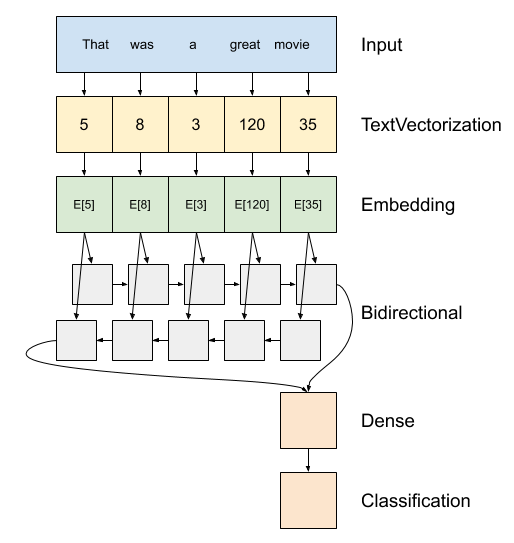
Arriba hay un diagrama del modelo.
Este modelo se puede construir como un
tf.keras.Sequential.La primera capa es la
encoder, que convierte el texto en una secuencia de índices de tokens.Después del codificador hay una capa de incrustación. Una capa de incrustación almacena un vector por palabra. Cuando se llama, convierte las secuencias de índices de palabras en secuencias de vectores. Estos vectores se pueden entrenar. Después del entrenamiento (con suficientes datos), las palabras con significados similares a menudo tienen vectores similares.
Este índice de búsqueda es mucho más eficiente que la operación equivalente de pasar un vector codificada de una sola caliente a través de un
tf.keras.layers.Densecapa.Una red neuronal recurrente (RNN) procesa la entrada de secuencia iterando a través de los elementos. Los RNN pasan las salidas de un paso de tiempo a su entrada en el siguiente paso de tiempo.
El
tf.keras.layers.Bidirectionalenvoltura también se puede utilizar con una capa RNN. Esto propaga la entrada hacia adelante y hacia atrás a través de la capa RNN y luego concatena la salida final.La principal ventaja de un RNN bidireccional es que la señal desde el principio de la entrada no necesita procesarse hasta el final en cada paso de tiempo para afectar la salida.
La principal desventaja de un RNN bidireccional es que no puede transmitir predicciones de manera eficiente a medida que se agregan palabras al final.
Después de la RNN ha convertido la secuencia para un único vector de los dos
layers.Densehacer algo de procesamiento final, y convertir de esta representación vectorial a un solo logit como la salida de clasificación.
El código para implementar esto es el siguiente:
model = tf.keras.Sequential([
    encoder,
    tf.keras.layers.Embedding(
        input_dim=len(encoder.get_vocabulary()),
        output_dim=64,
        # Use masking to handle the variable sequence lengths
        mask_zero=True),
    tf.keras.layers.Bidirectional(tf.keras.layers.LSTM(64)),
    tf.keras.layers.Dense(64, activation='relu'),
    tf.keras.layers.Dense(1)
])
Tenga en cuenta que el modelo secuencial de Keras se utiliza aquí, ya que todas las capas del modelo solo tienen una entrada y producen una salida única. En caso de que desee utilizar la capa RNN con estado, es posible que desee crear su modelo con la API funcional de Keras o la subclasificación del modelo para poder recuperar y reutilizar los estados de la capa RNN. Por favor, compruebe guía Keras RNN para más detalles.
Los capa de encaje usos de enmascaramiento para manejar la secuencia variable longitudes. Todas las capas después de la Embedding enmascaramiento de apoyo:
print([layer.supports_masking for layer in model.layers])
[False, True, True, True, True]
Para confirmar que esto funciona como se esperaba, evalúe una oración dos veces. Primero, solo para que no haya relleno para enmascarar:
# predict on a sample text without padding.

sample_text = ('The movie was cool. The animation and the graphics '
               'were out of this world. I would recommend this movie.')
predictions = model.predict(np.array([sample_text]))
print(predictions[0])
[-0.00012211]
Ahora, evalúelo nuevamente en un lote con una oración más larga. El resultado debería ser idéntico:
# predict on a sample text with padding

padding = "the " * 2000
predictions = model.predict(np.array([sample_text, padding]))
print(predictions[0])
[-0.00012211]
Compile el modelo de Keras para configurar el proceso de entrenamiento:
model.compile(loss=tf.keras.losses.BinaryCrossentropy(from_logits=True),
              optimizer=tf.keras.optimizers.Adam(1e-4),
              metrics=['accuracy'])
Entrena el modelo
history = model.fit(train_dataset, epochs=10,
                    validation_data=test_dataset,
                    validation_steps=30)
Epoch 1/10
391/391 [==============================] - 39s 84ms/step - loss: 0.6454 - accuracy: 0.5630 - val_loss: 0.4888 - val_accuracy: 0.7568
Epoch 2/10
391/391 [==============================] - 30s 75ms/step - loss: 0.3925 - accuracy: 0.8200 - val_loss: 0.3663 - val_accuracy: 0.8464
Epoch 3/10
391/391 [==============================] - 30s 75ms/step - loss: 0.3319 - accuracy: 0.8525 - val_loss: 0.3402 - val_accuracy: 0.8385
Epoch 4/10
391/391 [==============================] - 30s 75ms/step - loss: 0.3183 - accuracy: 0.8616 - val_loss: 0.3289 - val_accuracy: 0.8438
Epoch 5/10
391/391 [==============================] - 30s 75ms/step - loss: 0.3088 - accuracy: 0.8656 - val_loss: 0.3254 - val_accuracy: 0.8646
Epoch 6/10
391/391 [==============================] - 32s 81ms/step - loss: 0.3043 - accuracy: 0.8686 - val_loss: 0.3242 - val_accuracy: 0.8521
Epoch 7/10
391/391 [==============================] - 30s 76ms/step - loss: 0.3019 - accuracy: 0.8696 - val_loss: 0.3315 - val_accuracy: 0.8609
Epoch 8/10
391/391 [==============================] - 32s 76ms/step - loss: 0.3007 - accuracy: 0.8688 - val_loss: 0.3245 - val_accuracy: 0.8609
Epoch 9/10
391/391 [==============================] - 31s 77ms/step - loss: 0.2981 - accuracy: 0.8707 - val_loss: 0.3294 - val_accuracy: 0.8599
Epoch 10/10
391/391 [==============================] - 31s 78ms/step - loss: 0.2969 - accuracy: 0.8742 - val_loss: 0.3218 - val_accuracy: 0.8547
test_loss, test_acc = model.evaluate(test_dataset)

print('Test Loss:', test_loss)
print('Test Accuracy:', test_acc)
391/391 [==============================] - 15s 38ms/step - loss: 0.3185 - accuracy: 0.8582
Test Loss: 0.3184521794319153
Test Accuracy: 0.8581600189208984
plt.figure(figsize=(16, 8))
plt.subplot(1, 2, 1)
plot_graphs(history, 'accuracy')
plt.ylim(None, 1)
plt.subplot(1, 2, 2)
plot_graphs(history, 'loss')
plt.ylim(0, None)
(0.0, 0.6627909764647484)

Ejecute una predicción en una nueva oración:
Si la predicción es> = 0.0, es positiva, de lo contrario es negativa.
sample_text = ('The movie was cool. The animation and the graphics '
               'were out of this world. I would recommend this movie.')
predictions = model.predict(np.array([sample_text]))
Apila dos o más capas de LSTM
Capas recurrentes Keras tienen dos modos disponibles que son controlados por el return_sequences argumento del constructor:
Si
Falsedevuelve sólo el último de salida para cada secuencia de entrada (un tensor 2D de forma (batch_size, output_features)). Este es el predeterminado, utilizado en el modelo anterior.Si
Truese devuelven las secuencias completas de salidas sucesivas para cada paso de tiempo (un tensor 3D de la forma(batch_size, timesteps, output_features)).
Esto es lo que el flujo de información como se ve con return_sequences=True :
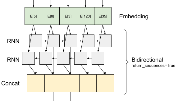
Lo interesante acerca del uso de un RNN con return_sequences=True es que la salida todavía tiene 3 ejes, como la entrada, por lo que se puede pasar a otra capa RNN, como este:
model = tf.keras.Sequential([
    encoder,
    tf.keras.layers.Embedding(len(encoder.get_vocabulary()), 64, mask_zero=True),
    tf.keras.layers.Bidirectional(tf.keras.layers.LSTM(64,  return_sequences=True)),
    tf.keras.layers.Bidirectional(tf.keras.layers.LSTM(32)),
    tf.keras.layers.Dense(64, activation='relu'),
    tf.keras.layers.Dropout(0.5),
    tf.keras.layers.Dense(1)
])
model.compile(loss=tf.keras.losses.BinaryCrossentropy(from_logits=True),
              optimizer=tf.keras.optimizers.Adam(1e-4),
              metrics=['accuracy'])
history = model.fit(train_dataset, epochs=10,
                    validation_data=test_dataset,
                    validation_steps=30)
Epoch 1/10
391/391 [==============================] - 71s 149ms/step - loss: 0.6502 - accuracy: 0.5625 - val_loss: 0.4923 - val_accuracy: 0.7573
Epoch 2/10
391/391 [==============================] - 55s 138ms/step - loss: 0.4067 - accuracy: 0.8198 - val_loss: 0.3727 - val_accuracy: 0.8271
Epoch 3/10
391/391 [==============================] - 54s 136ms/step - loss: 0.3417 - accuracy: 0.8543 - val_loss: 0.3343 - val_accuracy: 0.8510
Epoch 4/10
391/391 [==============================] - 53s 134ms/step - loss: 0.3242 - accuracy: 0.8607 - val_loss: 0.3268 - val_accuracy: 0.8568
Epoch 5/10
391/391 [==============================] - 53s 135ms/step - loss: 0.3174 - accuracy: 0.8652 - val_loss: 0.3213 - val_accuracy: 0.8516
Epoch 6/10
391/391 [==============================] - 52s 132ms/step - loss: 0.3098 - accuracy: 0.8671 - val_loss: 0.3294 - val_accuracy: 0.8547
Epoch 7/10
391/391 [==============================] - 53s 134ms/step - loss: 0.3063 - accuracy: 0.8697 - val_loss: 0.3158 - val_accuracy: 0.8594
Epoch 8/10
391/391 [==============================] - 52s 132ms/step - loss: 0.3043 - accuracy: 0.8692 - val_loss: 0.3184 - val_accuracy: 0.8521
Epoch 9/10
391/391 [==============================] - 53s 133ms/step - loss: 0.3016 - accuracy: 0.8704 - val_loss: 0.3208 - val_accuracy: 0.8609
Epoch 10/10
391/391 [==============================] - 54s 136ms/step - loss: 0.2975 - accuracy: 0.8740 - val_loss: 0.3301 - val_accuracy: 0.8651
test_loss, test_acc = model.evaluate(test_dataset)

print('Test Loss:', test_loss)
print('Test Accuracy:', test_acc)
391/391 [==============================] - 26s 65ms/step - loss: 0.3293 - accuracy: 0.8646
Test Loss: 0.329334557056427
Test Accuracy: 0.8646399974822998
# predict on a sample text without padding.

sample_text = ('The movie was not good. The animation and the graphics '
               'were terrible. I would not recommend this movie.')
predictions = model.predict(np.array([sample_text]))
print(predictions)
[[-1.6796288]]
plt.figure(figsize=(16, 6))
plt.subplot(1, 2, 1)
plot_graphs(history, 'accuracy')
plt.subplot(1, 2, 2)
plot_graphs(history, 'loss')

Echa un vistazo a otras capas recurrentes existentes, tales como capas GRU .
Si usted está en la construcción de interestied RNNs personalizados, consulte la Guía de Keras RNN .