
| | |  Посмотреть исходный код на GitHub Посмотреть исходный код на GitHub |
В этом учебном пособии модель Transformer обучается переводу набора данных с португальского на английский . Это расширенный пример, который предполагает знание генерации текста и внимания .
Основная идея модели Transformer — это самовнимание — способность обращать внимание на различные позиции входной последовательности для вычисления представления этой последовательности. Трансформатор создает стопки слоев собственного внимания и объясняется ниже в разделах Масштабированное скалярное произведение внимания и Внимание с несколькими головками .
Модель преобразователя обрабатывает входные данные переменного размера, используя стеки уровней внутреннего внимания вместо RNN или CNN . Эта общая архитектура имеет ряд преимуществ:
- Он не делает никаких предположений о временных/пространственных отношениях между данными. Это идеально подходит для обработки набора объектов (например, юнитов StarCraft ).
- Выходные данные слоя можно вычислять параллельно, а не последовательно, как RNN.
- Удаленные элементы могут влиять на вывод друг друга, не проходя через множество шагов RNN или слоев свертки (см., например, Преобразователь памяти сцен ).
- Он может изучать долгосрочные зависимости. Это проблема во многих задачах последовательности.
Недостатки этой архитектуры:
- Для временного ряда выходные данные для временного шага рассчитываются из всей истории , а не только из входных данных и текущего скрытого состояния. Это может быть менее эффективно.
- Если входные данные имеют временное/пространственное отношение, например текст, необходимо добавить некоторое позиционное кодирование, иначе модель фактически увидит набор слов.
После обучения модели в этой записной книжке вы сможете ввести предложение на португальском языке и вернуть перевод на английский язык.
Настраивать
pip install tensorflow_datasetspip install -U tensorflow-text
import collections
import logging
import os
import pathlib
import re
import string
import sys
import time

import numpy as np
import matplotlib.pyplot as plt

import tensorflow_datasets as tfds
import tensorflow_text as text
import tensorflow as tf
logging.getLogger('tensorflow').setLevel(logging.ERROR) # suppress warnings
Скачать набор данных
Используйте наборы данных TensorFlow для загрузки набора данных для перевода с португальского на английский из проекта TED Talks Open Translation Project .
Этот набор данных содержит примерно 50 000 обучающих примеров, 1100 проверочных примеров и 2000 тестовых примеров.
examples, metadata = tfds.load('ted_hrlr_translate/pt_to_en', with_info=True,
                               as_supervised=True)
train_examples, val_examples = examples['train'], examples['validation']
Объект tf.data.Dataset , возвращаемый наборами данных TensorFlow, дает пары текстовых примеров:
for pt_examples, en_examples in train_examples.batch(3).take(1):
  for pt in pt_examples.numpy():
    print(pt.decode('utf-8'))

  print()

  for en in en_examples.numpy():
    print(en.decode('utf-8'))
e quando melhoramos a procura , tiramos a única vantagem da impressão , que é a serendipidade .
mas e se estes fatores fossem ativos ?
mas eles não tinham a curiosidade de me testar .

and when you improve searchability , you actually take away the one advantage of print , which is serendipity .
but what if it were active ?
but they did n't test for curiosity .
Текстовая токенизация и детокенизация
Вы не можете обучать модель непосредственно на тексте. Сначала текст необходимо преобразовать в числовое представление. Как правило, вы конвертируете текст в последовательности идентификаторов маркеров, которые используются в качестве индексов во встраивании.
Одна популярная реализация, показанная в учебнике по токенизатору подслов, создает токенизаторы подслов ( text.BertTokenizer ), оптимизированные для этого набора данных, и экспортирует их в save_model .
Загрузите и разархивируйте и импортируйте saved_model :
model_name = "ted_hrlr_translate_pt_en_converter"
tf.keras.utils.get_file(
    f"{model_name}.zip",
    f"https://storage.googleapis.com/download.tensorflow.org/models/{model_name}.zip",
    cache_dir='.', cache_subdir='', extract=True
)
Downloading data from https://storage.googleapis.com/download.tensorflow.org/models/ted_hrlr_translate_pt_en_converter.zip
188416/184801 [==============================] - 0s 0us/step
196608/184801 [===============================] - 0s 0us/step
'./ted_hrlr_translate_pt_en_converter.zip'
tokenizers = tf.saved_model.load(model_name)
tf.saved_model содержит два токенизатора текста, один для английского и один для португальского языков. Оба имеют одинаковые методы:
[item for item in dir(tokenizers.en) if not item.startswith('_')]
['detokenize',
 'get_reserved_tokens',
 'get_vocab_path',
 'get_vocab_size',
 'lookup',
 'tokenize',
 'tokenizer',
 'vocab']
Метод tokenize преобразует пакет строк в дополненный пакет идентификаторов маркеров. Этот метод разделяет знаки препинания, строчные буквы и нормализует входные данные перед токенизацией. Эта стандартизация здесь не видна, потому что входные данные уже стандартизированы.
for en in en_examples.numpy():
  print(en.decode('utf-8'))
and when you improve searchability , you actually take away the one advantage of print , which is serendipity .
but what if it were active ?
but they did n't test for curiosity .
encoded = tokenizers.en.tokenize(en_examples)

for row in encoded.to_list():
  print(row)
[2, 72, 117, 79, 1259, 1491, 2362, 13, 79, 150, 184, 311, 71, 103, 2308, 74, 2679, 13, 148, 80, 55, 4840, 1434, 2423, 540, 15, 3]
[2, 87, 90, 107, 76, 129, 1852, 30, 3]
[2, 87, 83, 149, 50, 9, 56, 664, 85, 2512, 15, 3]
Метод detokenize пытается преобразовать эти идентификаторы токенов обратно в удобочитаемый текст:
round_trip = tokenizers.en.detokenize(encoded)
for line in round_trip.numpy():
  print(line.decode('utf-8'))
and when you improve searchability , you actually take away the one advantage of print , which is serendipity .
but what if it were active ?
but they did n ' t test for curiosity .
Метод lookup нижнего уровня преобразует идентификаторы токенов в текст токена:
tokens = tokenizers.en.lookup(encoded)
tokens
<tf.RaggedTensor [[b'[START]', b'and', b'when', b'you', b'improve', b'search', b'##ability',
  b',', b'you', b'actually', b'take', b'away', b'the', b'one', b'advantage',
  b'of', b'print', b',', b'which', b'is', b's', b'##ere', b'##nd', b'##ip',
  b'##ity', b'.', b'[END]']                                                 ,
 [b'[START]', b'but', b'what', b'if', b'it', b'were', b'active', b'?',
  b'[END]']                                                           ,
 [b'[START]', b'but', b'they', b'did', b'n', b"'", b't', b'test', b'for',
  b'curiosity', b'.', b'[END]']                                          ]>
Здесь вы можете увидеть «подсловный» аспект токенизаторов. Слово "поисковая способность" раскладывается на "поиск ##способность", а слово "интуитивная прозорливость" на "s ##ere ##nd ##ip ##ity"
Настройка входного конвейера
Чтобы построить входной конвейер, подходящий для обучения, вы примените некоторые преобразования к набору данных.
Эта функция будет использоваться для кодирования пакетов необработанного текста:
def tokenize_pairs(pt, en):
    pt = tokenizers.pt.tokenize(pt)
    # Convert from ragged to dense, padding with zeros.
    pt = pt.to_tensor()

    en = tokenizers.en.tokenize(en)
    # Convert from ragged to dense, padding with zeros.
    en = en.to_tensor()
    return pt, en
Вот простой конвейер ввода, который обрабатывает, перемешивает и группирует данные:
BUFFER_SIZE = 20000
BATCH_SIZE = 64
def make_batches(ds):
  return (
      ds
      .cache()
      .shuffle(BUFFER_SIZE)
      .batch(BATCH_SIZE)
      .map(tokenize_pairs, num_parallel_calls=tf.data.AUTOTUNE)
      .prefetch(tf.data.AUTOTUNE))


train_batches = make_batches(train_examples)
val_batches = make_batches(val_examples)
Позиционное кодирование
Слои внимания видят свои входные данные как набор векторов без последовательного порядка. Эта модель также не содержит рекуррентных или сверточных слоев. Из-за этого добавляется «позиционное кодирование», чтобы дать модели некоторую информацию об относительном положении токенов в предложении.
Вектор позиционного кодирования добавляется к вектору встраивания. Вложения представляют токен в d-мерном пространстве, где токены со схожим значением будут ближе друг к другу. Но вложения не кодируют относительное положение токенов в предложении. Таким образом, после добавления позиционного кодирования токены будут ближе друг к другу на основе схожести их значения и их положения в предложении , в d-мерном пространстве.
Формула для расчета позиционного кодирования выглядит следующим образом:
\[\Large{PE_{(pos, 2i)} = \sin(pos / 10000^{2i / d_{model} })} \]
\[\Large{PE_{(pos, 2i+1)} = \cos(pos / 10000^{2i / d_{model} })} \]
def get_angles(pos, i, d_model):
  angle_rates = 1 / np.power(10000, (2 * (i//2)) / np.float32(d_model))
  return pos * angle_rates
def positional_encoding(position, d_model):
  angle_rads = get_angles(np.arange(position)[:, np.newaxis],
                          np.arange(d_model)[np.newaxis, :],
                          d_model)

  # apply sin to even indices in the array; 2i
  angle_rads[:, 0::2] = np.sin(angle_rads[:, 0::2])

  # apply cos to odd indices in the array; 2i+1
  angle_rads[:, 1::2] = np.cos(angle_rads[:, 1::2])

  pos_encoding = angle_rads[np.newaxis, ...]

  return tf.cast(pos_encoding, dtype=tf.float32)
n, d = 2048, 512
pos_encoding = positional_encoding(n, d)
print(pos_encoding.shape)
pos_encoding = pos_encoding[0]

# Juggle the dimensions for the plot
pos_encoding = tf.reshape(pos_encoding, (n, d//2, 2))
pos_encoding = tf.transpose(pos_encoding, (2, 1, 0))
pos_encoding = tf.reshape(pos_encoding, (d, n))

plt.pcolormesh(pos_encoding, cmap='RdBu')
plt.ylabel('Depth')
plt.xlabel('Position')
plt.colorbar()
plt.show()
(1, 2048, 512)

Маскировка
Замаскируйте все маркеры пэдов в пакете последовательности. Это гарантирует, что модель не обрабатывает отступы как входные данные. Маска указывает, где присутствует значение пэда 0 : она выводит 1 в этих местах и 0 в противном случае.
def create_padding_mask(seq):
  seq = tf.cast(tf.math.equal(seq, 0), tf.float32)

  # add extra dimensions to add the padding
  # to the attention logits.
  return seq[:, tf.newaxis, tf.newaxis, :]  # (batch_size, 1, 1, seq_len)
x = tf.constant([[7, 6, 0, 0, 1], [1, 2, 3, 0, 0], [0, 0, 0, 4, 5]])
create_padding_mask(x)
<tf.Tensor: shape=(3, 1, 1, 5), dtype=float32, numpy=
array([[[[0., 0., 1., 1., 0.]]],


       [[[0., 0., 0., 1., 1.]]],


       [[[1., 1., 1., 0., 0.]]]], dtype=float32)>
Упреждающая маска используется для маскирования будущих токенов в последовательности. Другими словами, маска указывает, какие записи не следует использовать.
Это означает, что для предсказания третьего токена будут использоваться только первый и второй токен. Точно так же для прогнозирования четвертого токена будут использоваться только первый, второй и третий токены и так далее.
def create_look_ahead_mask(size):
  mask = 1 - tf.linalg.band_part(tf.ones((size, size)), -1, 0)
  return mask  # (seq_len, seq_len)
x = tf.random.uniform((1, 3))
temp = create_look_ahead_mask(x.shape[1])
temp
<tf.Tensor: shape=(3, 3), dtype=float32, numpy=
array([[0., 1., 1.],
       [0., 0., 1.],
       [0., 0., 0.]], dtype=float32)>
Внимание к масштабируемому точечному произведению
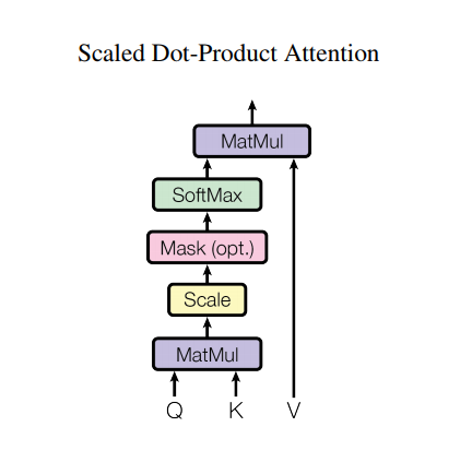
Функция внимания, используемая преобразователем, принимает три входа: Q (запрос), K (ключ), V (значение). Уравнение, используемое для расчета весов внимания, выглядит следующим образом:
\[\Large{Attention(Q, K, V) = softmax_k\left(\frac{QK^T}{\sqrt{d_k} }\right) V} \]
Скалярное произведение внимания масштабируется коэффициентом квадратного корня из глубины. Это делается потому, что для больших значений глубины скалярное произведение становится большим по величине, подталкивая функцию softmax, где она имеет небольшие градиенты, что приводит к очень жесткому softmax.
Например, предположим, что Q и K имеют среднее значение 0 и дисперсию 1. Их матричное умножение будет иметь среднее значение 0 и дисперсию dk . Таким образом, квадратный корень из dk используется для масштабирования, поэтому вы получаете постоянную дисперсию независимо от значения dk . Если дисперсия слишком низкая, выходные данные могут быть слишком плоскими для эффективной оптимизации. Если дисперсия слишком высока, softmax может насыщаться при инициализации, что затрудняет обучение.
Маска умножается на -1e9 (близко к отрицательной бесконечности). Это делается потому, что маска суммируется с масштабированным матричным умножением Q и K и применяется непосредственно перед softmax. Цель состоит в том, чтобы обнулить эти ячейки, а большие отрицательные входные данные для softmax близки к нулю на выходе.
def scaled_dot_product_attention(q, k, v, mask):
  """Calculate the attention weights.
  q, k, v must have matching leading dimensions.
  k, v must have matching penultimate dimension, i.e.: seq_len_k = seq_len_v.
  The mask has different shapes depending on its type(padding or look ahead)
  but it must be broadcastable for addition.

  Args:
    q: query shape == (..., seq_len_q, depth)
    k: key shape == (..., seq_len_k, depth)
    v: value shape == (..., seq_len_v, depth_v)
    mask: Float tensor with shape broadcastable
          to (..., seq_len_q, seq_len_k). Defaults to None.

  Returns:
    output, attention_weights
  """

  matmul_qk = tf.matmul(q, k, transpose_b=True)  # (..., seq_len_q, seq_len_k)

  # scale matmul_qk
  dk = tf.cast(tf.shape(k)[-1], tf.float32)
  scaled_attention_logits = matmul_qk / tf.math.sqrt(dk)

  # add the mask to the scaled tensor.
  if mask is not None:
    scaled_attention_logits += (mask * -1e9)

  # softmax is normalized on the last axis (seq_len_k) so that the scores
  # add up to 1.
  attention_weights = tf.nn.softmax(scaled_attention_logits, axis=-1)  # (..., seq_len_q, seq_len_k)

  output = tf.matmul(attention_weights, v)  # (..., seq_len_q, depth_v)

  return output, attention_weights
Поскольку нормализация softmax выполняется для K, ее значения определяют степень важности, придаваемую Q.
Выходные данные представляют собой произведение весов внимания и вектора V (значения). Это гарантирует, что токены, на которых вы хотите сосредоточиться, хранятся как есть, а ненужные токены удаляются.
def print_out(q, k, v):
  temp_out, temp_attn = scaled_dot_product_attention(
      q, k, v, None)
  print('Attention weights are:')
  print(temp_attn)
  print('Output is:')
  print(temp_out)
np.set_printoptions(suppress=True)

temp_k = tf.constant([[10, 0, 0],
                      [0, 10, 0],
                      [0, 0, 10],
                      [0, 0, 10]], dtype=tf.float32)  # (4, 3)

temp_v = tf.constant([[1, 0],
                      [10, 0],
                      [100, 5],
                      [1000, 6]], dtype=tf.float32)  # (4, 2)

# This `query` aligns with the second `key`,
# so the second `value` is returned.
temp_q = tf.constant([[0, 10, 0]], dtype=tf.float32)  # (1, 3)
print_out(temp_q, temp_k, temp_v)
Attention weights are:
tf.Tensor([[0. 1. 0. 0.]], shape=(1, 4), dtype=float32)
Output is:
tf.Tensor([[10.  0.]], shape=(1, 2), dtype=float32)
# This query aligns with a repeated key (third and fourth),
# so all associated values get averaged.
temp_q = tf.constant([[0, 0, 10]], dtype=tf.float32)  # (1, 3)
print_out(temp_q, temp_k, temp_v)
Attention weights are:
tf.Tensor([[0.  0.  0.5 0.5]], shape=(1, 4), dtype=float32)
Output is:
tf.Tensor([[550.    5.5]], shape=(1, 2), dtype=float32)
# This query aligns equally with the first and second key,
# so their values get averaged.
temp_q = tf.constant([[10, 10, 0]], dtype=tf.float32)  # (1, 3)
print_out(temp_q, temp_k, temp_v)
Attention weights are:
tf.Tensor([[0.5 0.5 0.  0. ]], shape=(1, 4), dtype=float32)
Output is:
tf.Tensor([[5.5 0. ]], shape=(1, 2), dtype=float32)
Передайте все запросы вместе.
temp_q = tf.constant([[0, 0, 10],
                      [0, 10, 0],
                      [10, 10, 0]], dtype=tf.float32)  # (3, 3)
print_out(temp_q, temp_k, temp_v)
Attention weights are:
tf.Tensor(
[[0.  0.  0.5 0.5]
 [0.  1.  0.  0. ]
 [0.5 0.5 0.  0. ]], shape=(3, 4), dtype=float32)
Output is:
tf.Tensor(
[[550.    5.5]
 [ 10.    0. ]
 [  5.5   0. ]], shape=(3, 2), dtype=float32)
Многоголовое внимание
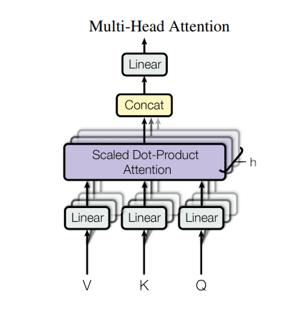
Многоголовое внимание состоит из четырех частей:
- Линейные слои.
- Масштабированное скалярное произведение внимания.
- Финальный линейный слой.
Каждый блок внимания с несколькими головками получает три входа; Q (запрос), K (ключ), V (значение). Они проходят через линейные (плотные) слои перед функцией многоголового внимания.
На приведенной выше диаграмме (K,Q,V) проходят через отдельные линейные ( Dense ) слои для каждой головы внимания. Для простоты/эффективности приведенный ниже код реализует это с использованием одного плотного слоя с числом выходов, умноженным на num_heads . Вывод преобразуется в форму (batch, num_heads, ...) перед применением функции внимания.
Определенная выше функция scaled_dot_product_attention применяется в одном вызове, широковещательном для эффективности. На этапе внимания необходимо использовать соответствующую маску. Затем вывод внимания для каждой головы объединяется (используя tf.transpose и tf.reshape ) и проходит через последний Dense слой.
Вместо одной головы внимания Q, K и V разделены на несколько головок, потому что это позволяет модели совместно обращать внимание на информацию из разных подпространств представления в разных позициях. После разделения каждая голова имеет уменьшенную размерность, поэтому общая стоимость вычислений такая же, как для внимания одной головы с полной размерностью.
class MultiHeadAttention(tf.keras.layers.Layer):
  def __init__(self, d_model, num_heads):
    super(MultiHeadAttention, self).__init__()
    self.num_heads = num_heads
    self.d_model = d_model

    assert d_model % self.num_heads == 0

    self.depth = d_model // self.num_heads

    self.wq = tf.keras.layers.Dense(d_model)
    self.wk = tf.keras.layers.Dense(d_model)
    self.wv = tf.keras.layers.Dense(d_model)

    self.dense = tf.keras.layers.Dense(d_model)

  def split_heads(self, x, batch_size):
    """Split the last dimension into (num_heads, depth).
    Transpose the result such that the shape is (batch_size, num_heads, seq_len, depth)
    """
    x = tf.reshape(x, (batch_size, -1, self.num_heads, self.depth))
    return tf.transpose(x, perm=[0, 2, 1, 3])

  def call(self, v, k, q, mask):
    batch_size = tf.shape(q)[0]

    q = self.wq(q)  # (batch_size, seq_len, d_model)
    k = self.wk(k)  # (batch_size, seq_len, d_model)
    v = self.wv(v)  # (batch_size, seq_len, d_model)

    q = self.split_heads(q, batch_size)  # (batch_size, num_heads, seq_len_q, depth)
    k = self.split_heads(k, batch_size)  # (batch_size, num_heads, seq_len_k, depth)
    v = self.split_heads(v, batch_size)  # (batch_size, num_heads, seq_len_v, depth)

    # scaled_attention.shape == (batch_size, num_heads, seq_len_q, depth)
    # attention_weights.shape == (batch_size, num_heads, seq_len_q, seq_len_k)
    scaled_attention, attention_weights = scaled_dot_product_attention(
        q, k, v, mask)

    scaled_attention = tf.transpose(scaled_attention, perm=[0, 2, 1, 3])  # (batch_size, seq_len_q, num_heads, depth)

    concat_attention = tf.reshape(scaled_attention,
                                  (batch_size, -1, self.d_model))  # (batch_size, seq_len_q, d_model)

    output = self.dense(concat_attention)  # (batch_size, seq_len_q, d_model)

    return output, attention_weights
Создайте слой MultiHeadAttention , чтобы попробовать. В каждом месте последовательности y MultiHeadAttention запускает все 8 головок внимания во всех других местах последовательности, возвращая новый вектор одинаковой длины в каждом месте.
temp_mha = MultiHeadAttention(d_model=512, num_heads=8)
y = tf.random.uniform((1, 60, 512))  # (batch_size, encoder_sequence, d_model)
out, attn = temp_mha(y, k=y, q=y, mask=None)
out.shape, attn.shape
(TensorShape([1, 60, 512]), TensorShape([1, 8, 60, 60]))
Сеть точечной прямой связи
Сеть точечной прямой связи состоит из двух полностью связанных слоев с активацией ReLU между ними.
def point_wise_feed_forward_network(d_model, dff):
  return tf.keras.Sequential([
      tf.keras.layers.Dense(dff, activation='relu'),  # (batch_size, seq_len, dff)
      tf.keras.layers.Dense(d_model)  # (batch_size, seq_len, d_model)
  ])
sample_ffn = point_wise_feed_forward_network(512, 2048)
sample_ffn(tf.random.uniform((64, 50, 512))).shape
TensorShape([64, 50, 512])
Кодер и декодер
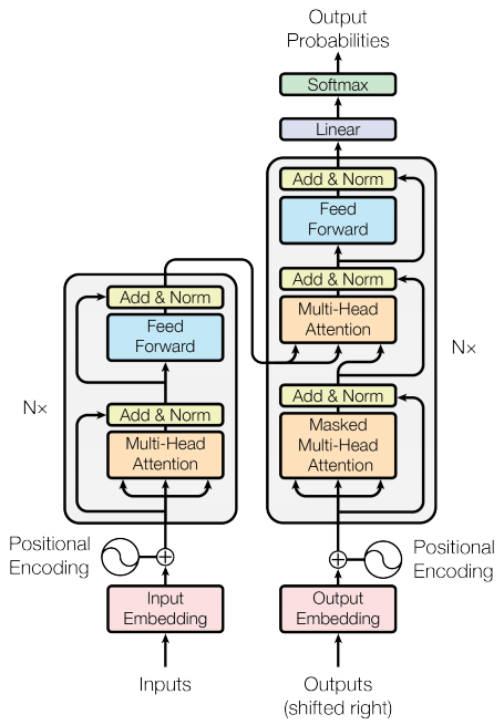
Модель преобразования следует тому же общему шаблону, что и стандартная последовательность для модели последовательности с вниманием .
- Входное предложение передается через
Nслоев кодировщика, который генерирует выходные данные для каждого токена в последовательности. - Декодер обращает внимание на выход кодировщика и свой собственный ввод (самовнимание), чтобы предсказать следующее слово.
Уровень кодировщика
Каждый уровень кодировщика состоит из подуровней:
- Многоголовое внимание (с маской-заглушкой)
- Точечные сети прямой связи.
Каждый из этих подслоев имеет остаточное соединение вокруг него, за которым следует нормализация слоя. Остаточные соединения помогают избежать проблемы исчезающего градиента в глубоких сетях.
Выход каждого подслоя — LayerNorm(x + Sublayer(x)) . Нормализация выполняется по d_model (последней). В преобразователе есть N слоев кодировщика.
class EncoderLayer(tf.keras.layers.Layer):
  def __init__(self, d_model, num_heads, dff, rate=0.1):
    super(EncoderLayer, self).__init__()

    self.mha = MultiHeadAttention(d_model, num_heads)
    self.ffn = point_wise_feed_forward_network(d_model, dff)

    self.layernorm1 = tf.keras.layers.LayerNormalization(epsilon=1e-6)
    self.layernorm2 = tf.keras.layers.LayerNormalization(epsilon=1e-6)

    self.dropout1 = tf.keras.layers.Dropout(rate)
    self.dropout2 = tf.keras.layers.Dropout(rate)

  def call(self, x, training, mask):

    attn_output, _ = self.mha(x, x, x, mask)  # (batch_size, input_seq_len, d_model)
    attn_output = self.dropout1(attn_output, training=training)
    out1 = self.layernorm1(x + attn_output)  # (batch_size, input_seq_len, d_model)

    ffn_output = self.ffn(out1)  # (batch_size, input_seq_len, d_model)
    ffn_output = self.dropout2(ffn_output, training=training)
    out2 = self.layernorm2(out1 + ffn_output)  # (batch_size, input_seq_len, d_model)

    return out2
sample_encoder_layer = EncoderLayer(512, 8, 2048)

sample_encoder_layer_output = sample_encoder_layer(
    tf.random.uniform((64, 43, 512)), False, None)

sample_encoder_layer_output.shape  # (batch_size, input_seq_len, d_model)
TensorShape([64, 43, 512])
Слой декодера
Каждый уровень декодера состоит из подуровней:
- Многоголовое внимание в маске (с маской упреждения и маской заполнения)
- Многоголовое внимание (с маской). V (значение) и K (клавиша) получают выходные данные энкодера в качестве входных данных. Q (запрос) получает выходные данные от маскированного подуровня внимания с несколькими головками.
- Сети с прямой поточечной связью
Каждый из этих подслоев имеет остаточное соединение вокруг него, за которым следует нормализация слоя. Выход каждого подслоя — LayerNorm(x + Sublayer(x)) . Нормализация выполняется по d_model (последней).
В преобразователе имеется N слоев декодера.
Поскольку Q получает выходные данные от первого блока внимания декодера, а K получает выходные данные кодировщика, веса внимания представляют важность, придаваемую входным данным декодера на основе выходных данных кодировщика. Другими словами, декодер предсказывает следующий токен, просматривая выходные данные кодировщика и самостоятельно обращаясь к своим собственным выводам. См. демонстрацию выше в разделе внимания масштабированного скалярного произведения.
class DecoderLayer(tf.keras.layers.Layer):
  def __init__(self, d_model, num_heads, dff, rate=0.1):
    super(DecoderLayer, self).__init__()

    self.mha1 = MultiHeadAttention(d_model, num_heads)
    self.mha2 = MultiHeadAttention(d_model, num_heads)

    self.ffn = point_wise_feed_forward_network(d_model, dff)

    self.layernorm1 = tf.keras.layers.LayerNormalization(epsilon=1e-6)
    self.layernorm2 = tf.keras.layers.LayerNormalization(epsilon=1e-6)
    self.layernorm3 = tf.keras.layers.LayerNormalization(epsilon=1e-6)

    self.dropout1 = tf.keras.layers.Dropout(rate)
    self.dropout2 = tf.keras.layers.Dropout(rate)
    self.dropout3 = tf.keras.layers.Dropout(rate)

  def call(self, x, enc_output, training,
           look_ahead_mask, padding_mask):
    # enc_output.shape == (batch_size, input_seq_len, d_model)

    attn1, attn_weights_block1 = self.mha1(x, x, x, look_ahead_mask)  # (batch_size, target_seq_len, d_model)
    attn1 = self.dropout1(attn1, training=training)
    out1 = self.layernorm1(attn1 + x)

    attn2, attn_weights_block2 = self.mha2(
        enc_output, enc_output, out1, padding_mask)  # (batch_size, target_seq_len, d_model)
    attn2 = self.dropout2(attn2, training=training)
    out2 = self.layernorm2(attn2 + out1)  # (batch_size, target_seq_len, d_model)

    ffn_output = self.ffn(out2)  # (batch_size, target_seq_len, d_model)
    ffn_output = self.dropout3(ffn_output, training=training)
    out3 = self.layernorm3(ffn_output + out2)  # (batch_size, target_seq_len, d_model)

    return out3, attn_weights_block1, attn_weights_block2
sample_decoder_layer = DecoderLayer(512, 8, 2048)

sample_decoder_layer_output, _, _ = sample_decoder_layer(
    tf.random.uniform((64, 50, 512)), sample_encoder_layer_output,
    False, None, None)

sample_decoder_layer_output.shape  # (batch_size, target_seq_len, d_model)
TensorShape([64, 50, 512])
Кодер
Encoder состоит из:
- Внедрение ввода
- Позиционное кодирование
- N слоев кодировщика
Вход проходит через вложение, которое суммируется с позиционным кодированием. Выход этого суммирования является входом для слоев кодировщика. Выход кодировщика является входом декодера.
class Encoder(tf.keras.layers.Layer):
  def __init__(self, num_layers, d_model, num_heads, dff, input_vocab_size,
               maximum_position_encoding, rate=0.1):
    super(Encoder, self).__init__()

    self.d_model = d_model
    self.num_layers = num_layers

    self.embedding = tf.keras.layers.Embedding(input_vocab_size, d_model)
    self.pos_encoding = positional_encoding(maximum_position_encoding,
                                            self.d_model)

    self.enc_layers = [EncoderLayer(d_model, num_heads, dff, rate)
                       for _ in range(num_layers)]

    self.dropout = tf.keras.layers.Dropout(rate)

  def call(self, x, training, mask):

    seq_len = tf.shape(x)[1]

    # adding embedding and position encoding.
    x = self.embedding(x)  # (batch_size, input_seq_len, d_model)
    x *= tf.math.sqrt(tf.cast(self.d_model, tf.float32))
    x += self.pos_encoding[:, :seq_len, :]

    x = self.dropout(x, training=training)

    for i in range(self.num_layers):
      x = self.enc_layers[i](x, training, mask)

    return x  # (batch_size, input_seq_len, d_model)
sample_encoder = Encoder(num_layers=2, d_model=512, num_heads=8,
                         dff=2048, input_vocab_size=8500,
                         maximum_position_encoding=10000)
temp_input = tf.random.uniform((64, 62), dtype=tf.int64, minval=0, maxval=200)

sample_encoder_output = sample_encoder(temp_input, training=False, mask=None)

print(sample_encoder_output.shape)  # (batch_size, input_seq_len, d_model)
(64, 62, 512)
Декодер
Decoder состоит из:
- Встраивание вывода
- Позиционное кодирование
- N слоев декодера
Цель проходит через вложение, которое суммируется с позиционным кодированием. Выход этого суммирования является входом для слоев декодера. Выход декодера является входом для конечного линейного слоя.
class Decoder(tf.keras.layers.Layer):
  def __init__(self, num_layers, d_model, num_heads, dff, target_vocab_size,
               maximum_position_encoding, rate=0.1):
    super(Decoder, self).__init__()

    self.d_model = d_model
    self.num_layers = num_layers

    self.embedding = tf.keras.layers.Embedding(target_vocab_size, d_model)
    self.pos_encoding = positional_encoding(maximum_position_encoding, d_model)

    self.dec_layers = [DecoderLayer(d_model, num_heads, dff, rate)
                       for _ in range(num_layers)]
    self.dropout = tf.keras.layers.Dropout(rate)

  def call(self, x, enc_output, training,
           look_ahead_mask, padding_mask):

    seq_len = tf.shape(x)[1]
    attention_weights = {}

    x = self.embedding(x)  # (batch_size, target_seq_len, d_model)
    x *= tf.math.sqrt(tf.cast(self.d_model, tf.float32))
    x += self.pos_encoding[:, :seq_len, :]

    x = self.dropout(x, training=training)

    for i in range(self.num_layers):
      x, block1, block2 = self.dec_layers[i](x, enc_output, training,
                                             look_ahead_mask, padding_mask)

      attention_weights[f'decoder_layer{i+1}_block1'] = block1
      attention_weights[f'decoder_layer{i+1}_block2'] = block2

    # x.shape == (batch_size, target_seq_len, d_model)
    return x, attention_weights
sample_decoder = Decoder(num_layers=2, d_model=512, num_heads=8,
                         dff=2048, target_vocab_size=8000,
                         maximum_position_encoding=5000)
temp_input = tf.random.uniform((64, 26), dtype=tf.int64, minval=0, maxval=200)

output, attn = sample_decoder(temp_input,
                              enc_output=sample_encoder_output,
                              training=False,
                              look_ahead_mask=None,
                              padding_mask=None)

output.shape, attn['decoder_layer2_block2'].shape
(TensorShape([64, 26, 512]), TensorShape([64, 8, 26, 62]))
Создайте Трансформера
Преобразователь состоит из кодера, декодера и конечного линейного слоя. Выход декодера является входом для линейного слоя, и его выход возвращается.
class Transformer(tf.keras.Model):
  def __init__(self, num_layers, d_model, num_heads, dff, input_vocab_size,
               target_vocab_size, pe_input, pe_target, rate=0.1):
    super().__init__()
    self.encoder = Encoder(num_layers, d_model, num_heads, dff,
                             input_vocab_size, pe_input, rate)

    self.decoder = Decoder(num_layers, d_model, num_heads, dff,
                           target_vocab_size, pe_target, rate)

    self.final_layer = tf.keras.layers.Dense(target_vocab_size)

  def call(self, inputs, training):
    # Keras models prefer if you pass all your inputs in the first argument
    inp, tar = inputs

    enc_padding_mask, look_ahead_mask, dec_padding_mask = self.create_masks(inp, tar)

    enc_output = self.encoder(inp, training, enc_padding_mask)  # (batch_size, inp_seq_len, d_model)

    # dec_output.shape == (batch_size, tar_seq_len, d_model)
    dec_output, attention_weights = self.decoder(
        tar, enc_output, training, look_ahead_mask, dec_padding_mask)

    final_output = self.final_layer(dec_output)  # (batch_size, tar_seq_len, target_vocab_size)

    return final_output, attention_weights

  def create_masks(self, inp, tar):
    # Encoder padding mask
    enc_padding_mask = create_padding_mask(inp)

    # Used in the 2nd attention block in the decoder.
    # This padding mask is used to mask the encoder outputs.
    dec_padding_mask = create_padding_mask(inp)

    # Used in the 1st attention block in the decoder.
    # It is used to pad and mask future tokens in the input received by
    # the decoder.
    look_ahead_mask = create_look_ahead_mask(tf.shape(tar)[1])
    dec_target_padding_mask = create_padding_mask(tar)
    look_ahead_mask = tf.maximum(dec_target_padding_mask, look_ahead_mask)

    return enc_padding_mask, look_ahead_mask, dec_padding_mask
sample_transformer = Transformer(
    num_layers=2, d_model=512, num_heads=8, dff=2048,
    input_vocab_size=8500, target_vocab_size=8000,
    pe_input=10000, pe_target=6000)

temp_input = tf.random.uniform((64, 38), dtype=tf.int64, minval=0, maxval=200)
temp_target = tf.random.uniform((64, 36), dtype=tf.int64, minval=0, maxval=200)

fn_out, _ = sample_transformer([temp_input, temp_target], training=False)

fn_out.shape  # (batch_size, tar_seq_len, target_vocab_size)
TensorShape([64, 36, 8000])
Установить гиперпараметры
Чтобы этот пример был небольшим и относительно быстрым, значения num_layers, d_model, dff были уменьшены.
Базовая модель, описанная в документе , использовала: num_layers=6, d_model=512, dff=2048 .
num_layers = 4
d_model = 128
dff = 512
num_heads = 8
dropout_rate = 0.1
Оптимизатор
Используйте оптимизатор Adam с настраиваемым планировщиком скорости обучения по формуле из статьи .
\[\Large{lrate = d_{model}^{-0.5} * \min(step{\_}num^{-0.5}, step{\_}num \cdot warmup{\_}steps^{-1.5})}\]
class CustomSchedule(tf.keras.optimizers.schedules.LearningRateSchedule):
  def __init__(self, d_model, warmup_steps=4000):
    super(CustomSchedule, self).__init__()

    self.d_model = d_model
    self.d_model = tf.cast(self.d_model, tf.float32)

    self.warmup_steps = warmup_steps

  def __call__(self, step):
    arg1 = tf.math.rsqrt(step)
    arg2 = step * (self.warmup_steps ** -1.5)

    return tf.math.rsqrt(self.d_model) * tf.math.minimum(arg1, arg2)
learning_rate = CustomSchedule(d_model)

optimizer = tf.keras.optimizers.Adam(learning_rate, beta_1=0.9, beta_2=0.98,
                                     epsilon=1e-9)
temp_learning_rate_schedule = CustomSchedule(d_model)

plt.plot(temp_learning_rate_schedule(tf.range(40000, dtype=tf.float32)))
plt.ylabel("Learning Rate")
plt.xlabel("Train Step")
Text(0.5, 0, 'Train Step')

Потери и показатели
Поскольку целевые последовательности дополняются, важно применять маску заполнения при расчете потерь.
loss_object = tf.keras.losses.SparseCategoricalCrossentropy(
    from_logits=True, reduction='none')
def loss_function(real, pred):
  mask = tf.math.logical_not(tf.math.equal(real, 0))
  loss_ = loss_object(real, pred)

  mask = tf.cast(mask, dtype=loss_.dtype)
  loss_ *= mask

  return tf.reduce_sum(loss_)/tf.reduce_sum(mask)


def accuracy_function(real, pred):
  accuracies = tf.equal(real, tf.argmax(pred, axis=2))

  mask = tf.math.logical_not(tf.math.equal(real, 0))
  accuracies = tf.math.logical_and(mask, accuracies)

  accuracies = tf.cast(accuracies, dtype=tf.float32)
  mask = tf.cast(mask, dtype=tf.float32)
  return tf.reduce_sum(accuracies)/tf.reduce_sum(mask)
train_loss = tf.keras.metrics.Mean(name='train_loss')
train_accuracy = tf.keras.metrics.Mean(name='train_accuracy')
Обучение и контрольно-пропускной пункт
transformer = Transformer(
    num_layers=num_layers,
    d_model=d_model,
    num_heads=num_heads,
    dff=dff,
    input_vocab_size=tokenizers.pt.get_vocab_size().numpy(),
    target_vocab_size=tokenizers.en.get_vocab_size().numpy(),
    pe_input=1000,
    pe_target=1000,
    rate=dropout_rate)
Создайте путь к контрольной точке и менеджер контрольных точек. Это будет использоваться для сохранения контрольных точек каждые n эпох.
checkpoint_path = "./checkpoints/train"

ckpt = tf.train.Checkpoint(transformer=transformer,
                           optimizer=optimizer)

ckpt_manager = tf.train.CheckpointManager(ckpt, checkpoint_path, max_to_keep=5)

# if a checkpoint exists, restore the latest checkpoint.
if ckpt_manager.latest_checkpoint:
  ckpt.restore(ckpt_manager.latest_checkpoint)
  print('Latest checkpoint restored!!')
Цель делится на tar_inp и tar_real. tar_inp передается в качестве входных данных декодеру. tar_real — это тот же ввод, сдвинутый на 1: в каждом месте в tar_input tar_real содержит следующий токен, который должен быть предсказан.
Например, sentence = "SOS Лев в джунглях спит EOS"
tar_inp = "SOS Лев в джунглях спит"
tar_real = "Лев в джунглях спит EOS"
Трансформатор — это авторегрессивная модель: он делает прогнозы по частям и использует свои выходные данные, чтобы решить, что делать дальше.
Во время обучения в этом примере используется принуждение учителя (как в учебнике по генерации текста ). Принуждение учителя передает истинный вывод на следующий временной шаг независимо от того, что модель предсказывает на текущем временном шаге.
По мере того, как преобразователь предсказывает каждую лексему, внутреннее внимание позволяет ему просмотреть предыдущие лексемы во входной последовательности, чтобы лучше предсказать следующую лексему.
Чтобы модель не заглядывала в ожидаемый результат, модель использует упреждающую маску.
EPOCHS = 20
# The @tf.function trace-compiles train_step into a TF graph for faster
# execution. The function specializes to the precise shape of the argument
# tensors. To avoid re-tracing due to the variable sequence lengths or variable
# batch sizes (the last batch is smaller), use input_signature to specify
# more generic shapes.

train_step_signature = [
    tf.TensorSpec(shape=(None, None), dtype=tf.int64),
    tf.TensorSpec(shape=(None, None), dtype=tf.int64),
]


@tf.function(input_signature=train_step_signature)
def train_step(inp, tar):
  tar_inp = tar[:, :-1]
  tar_real = tar[:, 1:]

  with tf.GradientTape() as tape:
    predictions, _ = transformer([inp, tar_inp],
                                 training = True)
    loss = loss_function(tar_real, predictions)

  gradients = tape.gradient(loss, transformer.trainable_variables)
  optimizer.apply_gradients(zip(gradients, transformer.trainable_variables))

  train_loss(loss)
  train_accuracy(accuracy_function(tar_real, predictions))
Португальский язык используется в качестве языка ввода, а английский является целевым языком.
for epoch in range(EPOCHS):
  start = time.time()

  train_loss.reset_states()
  train_accuracy.reset_states()

  # inp -> portuguese, tar -> english
  for (batch, (inp, tar)) in enumerate(train_batches):
    train_step(inp, tar)

    if batch % 50 == 0:
      print(f'Epoch {epoch + 1} Batch {batch} Loss {train_loss.result():.4f} Accuracy {train_accuracy.result():.4f}')

  if (epoch + 1) % 5 == 0:
    ckpt_save_path = ckpt_manager.save()
    print(f'Saving checkpoint for epoch {epoch+1} at {ckpt_save_path}')

  print(f'Epoch {epoch + 1} Loss {train_loss.result():.4f} Accuracy {train_accuracy.result():.4f}')

  print(f'Time taken for 1 epoch: {time.time() - start:.2f} secs\n')
Epoch 1 Batch 0 Loss 8.8600 Accuracy 0.0000
Epoch 1 Batch 50 Loss 8.7935 Accuracy 0.0082
Epoch 1 Batch 100 Loss 8.6902 Accuracy 0.0273
Epoch 1 Batch 150 Loss 8.5769 Accuracy 0.0335
Epoch 1 Batch 200 Loss 8.4387 Accuracy 0.0365
Epoch 1 Batch 250 Loss 8.2718 Accuracy 0.0386
Epoch 1 Batch 300 Loss 8.0845 Accuracy 0.0412
Epoch 1 Batch 350 Loss 7.8877 Accuracy 0.0481
Epoch 1 Batch 400 Loss 7.7002 Accuracy 0.0552
Epoch 1 Batch 450 Loss 7.5304 Accuracy 0.0629
Epoch 1 Batch 500 Loss 7.3857 Accuracy 0.0702
Epoch 1 Batch 550 Loss 7.2542 Accuracy 0.0776
Epoch 1 Batch 600 Loss 7.1327 Accuracy 0.0851
Epoch 1 Batch 650 Loss 7.0164 Accuracy 0.0930
Epoch 1 Batch 700 Loss 6.9088 Accuracy 0.1003
Epoch 1 Batch 750 Loss 6.8080 Accuracy 0.1070
Epoch 1 Batch 800 Loss 6.7173 Accuracy 0.1129
Epoch 1 Loss 6.7021 Accuracy 0.1139
Time taken for 1 epoch: 58.85 secs

Epoch 2 Batch 0 Loss 5.2952 Accuracy 0.2221
Epoch 2 Batch 50 Loss 5.2513 Accuracy 0.2094
Epoch 2 Batch 100 Loss 5.2103 Accuracy 0.2140
Epoch 2 Batch 150 Loss 5.1780 Accuracy 0.2176
Epoch 2 Batch 200 Loss 5.1436 Accuracy 0.2218
Epoch 2 Batch 250 Loss 5.1173 Accuracy 0.2246
Epoch 2 Batch 300 Loss 5.0939 Accuracy 0.2269
Epoch 2 Batch 350 Loss 5.0719 Accuracy 0.2295
Epoch 2 Batch 400 Loss 5.0508 Accuracy 0.2318
Epoch 2 Batch 450 Loss 5.0308 Accuracy 0.2337
Epoch 2 Batch 500 Loss 5.0116 Accuracy 0.2353
Epoch 2 Batch 550 Loss 4.9897 Accuracy 0.2376
Epoch 2 Batch 600 Loss 4.9701 Accuracy 0.2394
Epoch 2 Batch 650 Loss 4.9543 Accuracy 0.2407
Epoch 2 Batch 700 Loss 4.9345 Accuracy 0.2425
Epoch 2 Batch 750 Loss 4.9169 Accuracy 0.2442
Epoch 2 Batch 800 Loss 4.9007 Accuracy 0.2455
Epoch 2 Loss 4.8988 Accuracy 0.2456
Time taken for 1 epoch: 45.69 secs

Epoch 3 Batch 0 Loss 4.7236 Accuracy 0.2578
Epoch 3 Batch 50 Loss 4.5860 Accuracy 0.2705
Epoch 3 Batch 100 Loss 4.5758 Accuracy 0.2723
Epoch 3 Batch 150 Loss 4.5789 Accuracy 0.2728
Epoch 3 Batch 200 Loss 4.5699 Accuracy 0.2737
Epoch 3 Batch 250 Loss 4.5529 Accuracy 0.2753
Epoch 3 Batch 300 Loss 4.5462 Accuracy 0.2753
Epoch 3 Batch 350 Loss 4.5377 Accuracy 0.2762
Epoch 3 Batch 400 Loss 4.5301 Accuracy 0.2764
Epoch 3 Batch 450 Loss 4.5155 Accuracy 0.2776
Epoch 3 Batch 500 Loss 4.5036 Accuracy 0.2787
Epoch 3 Batch 550 Loss 4.4950 Accuracy 0.2794
Epoch 3 Batch 600 Loss 4.4860 Accuracy 0.2804
Epoch 3 Batch 650 Loss 4.4753 Accuracy 0.2814
Epoch 3 Batch 700 Loss 4.4643 Accuracy 0.2823
Epoch 3 Batch 750 Loss 4.4530 Accuracy 0.2837
Epoch 3 Batch 800 Loss 4.4401 Accuracy 0.2852
Epoch 3 Loss 4.4375 Accuracy 0.2855
Time taken for 1 epoch: 45.96 secs

Epoch 4 Batch 0 Loss 3.9880 Accuracy 0.3285
Epoch 4 Batch 50 Loss 4.1496 Accuracy 0.3146
Epoch 4 Batch 100 Loss 4.1353 Accuracy 0.3146
Epoch 4 Batch 150 Loss 4.1263 Accuracy 0.3153
Epoch 4 Batch 200 Loss 4.1171 Accuracy 0.3165
Epoch 4 Batch 250 Loss 4.1144 Accuracy 0.3169
Epoch 4 Batch 300 Loss 4.0976 Accuracy 0.3190
Epoch 4 Batch 350 Loss 4.0848 Accuracy 0.3206
Epoch 4 Batch 400 Loss 4.0703 Accuracy 0.3228
Epoch 4 Batch 450 Loss 4.0569 Accuracy 0.3247
Epoch 4 Batch 500 Loss 4.0429 Accuracy 0.3265
Epoch 4 Batch 550 Loss 4.0231 Accuracy 0.3291
Epoch 4 Batch 600 Loss 4.0075 Accuracy 0.3311
Epoch 4 Batch 650 Loss 3.9933 Accuracy 0.3331
Epoch 4 Batch 700 Loss 3.9778 Accuracy 0.3353
Epoch 4 Batch 750 Loss 3.9625 Accuracy 0.3375
Epoch 4 Batch 800 Loss 3.9505 Accuracy 0.3393
Epoch 4 Loss 3.9483 Accuracy 0.3397
Time taken for 1 epoch: 45.59 secs

Epoch 5 Batch 0 Loss 3.7342 Accuracy 0.3712
Epoch 5 Batch 50 Loss 3.5723 Accuracy 0.3851
Epoch 5 Batch 100 Loss 3.5656 Accuracy 0.3861
Epoch 5 Batch 150 Loss 3.5706 Accuracy 0.3857
Epoch 5 Batch 200 Loss 3.5701 Accuracy 0.3863
Epoch 5 Batch 250 Loss 3.5621 Accuracy 0.3877
Epoch 5 Batch 300 Loss 3.5527 Accuracy 0.3887
Epoch 5 Batch 350 Loss 3.5429 Accuracy 0.3904
Epoch 5 Batch 400 Loss 3.5318 Accuracy 0.3923
Epoch 5 Batch 450 Loss 3.5238 Accuracy 0.3937
Epoch 5 Batch 500 Loss 3.5141 Accuracy 0.3949
Epoch 5 Batch 550 Loss 3.5066 Accuracy 0.3958
Epoch 5 Batch 600 Loss 3.4956 Accuracy 0.3974
Epoch 5 Batch 650 Loss 3.4876 Accuracy 0.3986
Epoch 5 Batch 700 Loss 3.4788 Accuracy 0.4000
Epoch 5 Batch 750 Loss 3.4676 Accuracy 0.4014
Epoch 5 Batch 800 Loss 3.4590 Accuracy 0.4027
Saving checkpoint for epoch 5 at ./checkpoints/train/ckpt-1
Epoch 5 Loss 3.4583 Accuracy 0.4029
Time taken for 1 epoch: 46.04 secs

Epoch 6 Batch 0 Loss 3.0131 Accuracy 0.4610
Epoch 6 Batch 50 Loss 3.1403 Accuracy 0.4404
Epoch 6 Batch 100 Loss 3.1320 Accuracy 0.4422
Epoch 6 Batch 150 Loss 3.1314 Accuracy 0.4425
Epoch 6 Batch 200 Loss 3.1450 Accuracy 0.4411
Epoch 6 Batch 250 Loss 3.1438 Accuracy 0.4405
Epoch 6 Batch 300 Loss 3.1306 Accuracy 0.4424
Epoch 6 Batch 350 Loss 3.1161 Accuracy 0.4445
Epoch 6 Batch 400 Loss 3.1097 Accuracy 0.4453
Epoch 6 Batch 450 Loss 3.0983 Accuracy 0.4469
Epoch 6 Batch 500 Loss 3.0900 Accuracy 0.4483
Epoch 6 Batch 550 Loss 3.0816 Accuracy 0.4496
Epoch 6 Batch 600 Loss 3.0740 Accuracy 0.4507
Epoch 6 Batch 650 Loss 3.0695 Accuracy 0.4514
Epoch 6 Batch 700 Loss 3.0602 Accuracy 0.4528
Epoch 6 Batch 750 Loss 3.0528 Accuracy 0.4539
Epoch 6 Batch 800 Loss 3.0436 Accuracy 0.4553
Epoch 6 Loss 3.0425 Accuracy 0.4554
Time taken for 1 epoch: 46.13 secs

Epoch 7 Batch 0 Loss 2.7147 Accuracy 0.4940
Epoch 7 Batch 50 Loss 2.7671 Accuracy 0.4863
Epoch 7 Batch 100 Loss 2.7369 Accuracy 0.4934
Epoch 7 Batch 150 Loss 2.7562 Accuracy 0.4909
Epoch 7 Batch 200 Loss 2.7441 Accuracy 0.4926
Epoch 7 Batch 250 Loss 2.7464 Accuracy 0.4929
Epoch 7 Batch 300 Loss 2.7430 Accuracy 0.4932
Epoch 7 Batch 350 Loss 2.7342 Accuracy 0.4944
Epoch 7 Batch 400 Loss 2.7271 Accuracy 0.4954
Epoch 7 Batch 450 Loss 2.7215 Accuracy 0.4963
Epoch 7 Batch 500 Loss 2.7157 Accuracy 0.4972
Epoch 7 Batch 550 Loss 2.7123 Accuracy 0.4978
Epoch 7 Batch 600 Loss 2.7071 Accuracy 0.4985
Epoch 7 Batch 650 Loss 2.7038 Accuracy 0.4990
Epoch 7 Batch 700 Loss 2.6979 Accuracy 0.5002
Epoch 7 Batch 750 Loss 2.6946 Accuracy 0.5007
Epoch 7 Batch 800 Loss 2.6923 Accuracy 0.5013
Epoch 7 Loss 2.6913 Accuracy 0.5015
Time taken for 1 epoch: 46.02 secs

Epoch 8 Batch 0 Loss 2.3681 Accuracy 0.5459
Epoch 8 Batch 50 Loss 2.4812 Accuracy 0.5260
Epoch 8 Batch 100 Loss 2.4682 Accuracy 0.5294
Epoch 8 Batch 150 Loss 2.4743 Accuracy 0.5287
Epoch 8 Batch 200 Loss 2.4625 Accuracy 0.5303
Epoch 8 Batch 250 Loss 2.4627 Accuracy 0.5303
Epoch 8 Batch 300 Loss 2.4624 Accuracy 0.5308
Epoch 8 Batch 350 Loss 2.4586 Accuracy 0.5314
Epoch 8 Batch 400 Loss 2.4532 Accuracy 0.5324
Epoch 8 Batch 450 Loss 2.4530 Accuracy 0.5326
Epoch 8 Batch 500 Loss 2.4508 Accuracy 0.5330
Epoch 8 Batch 550 Loss 2.4481 Accuracy 0.5338
Epoch 8 Batch 600 Loss 2.4455 Accuracy 0.5343
Epoch 8 Batch 650 Loss 2.4427 Accuracy 0.5348
Epoch 8 Batch 700 Loss 2.4399 Accuracy 0.5352
Epoch 8 Batch 750 Loss 2.4392 Accuracy 0.5353
Epoch 8 Batch 800 Loss 2.4367 Accuracy 0.5358
Epoch 8 Loss 2.4357 Accuracy 0.5360
Time taken for 1 epoch: 45.31 secs

Epoch 9 Batch 0 Loss 2.1790 Accuracy 0.5595
Epoch 9 Batch 50 Loss 2.2201 Accuracy 0.5676
Epoch 9 Batch 100 Loss 2.2420 Accuracy 0.5629
Epoch 9 Batch 150 Loss 2.2444 Accuracy 0.5623
Epoch 9 Batch 200 Loss 2.2535 Accuracy 0.5610
Epoch 9 Batch 250 Loss 2.2562 Accuracy 0.5603
Epoch 9 Batch 300 Loss 2.2572 Accuracy 0.5603
Epoch 9 Batch 350 Loss 2.2646 Accuracy 0.5592
Epoch 9 Batch 400 Loss 2.2624 Accuracy 0.5597
Epoch 9 Batch 450 Loss 2.2595 Accuracy 0.5601
Epoch 9 Batch 500 Loss 2.2598 Accuracy 0.5600
Epoch 9 Batch 550 Loss 2.2590 Accuracy 0.5602
Epoch 9 Batch 600 Loss 2.2563 Accuracy 0.5607
Epoch 9 Batch 650 Loss 2.2578 Accuracy 0.5606
Epoch 9 Batch 700 Loss 2.2550 Accuracy 0.5611
Epoch 9 Batch 750 Loss 2.2536 Accuracy 0.5614
Epoch 9 Batch 800 Loss 2.2511 Accuracy 0.5618
Epoch 9 Loss 2.2503 Accuracy 0.5620
Time taken for 1 epoch: 44.87 secs

Epoch 10 Batch 0 Loss 2.0921 Accuracy 0.5928
Epoch 10 Batch 50 Loss 2.1196 Accuracy 0.5788
Epoch 10 Batch 100 Loss 2.0969 Accuracy 0.5828
Epoch 10 Batch 150 Loss 2.0954 Accuracy 0.5834
Epoch 10 Batch 200 Loss 2.0965 Accuracy 0.5827
Epoch 10 Batch 250 Loss 2.1029 Accuracy 0.5822
Epoch 10 Batch 300 Loss 2.0999 Accuracy 0.5827
Epoch 10 Batch 350 Loss 2.1007 Accuracy 0.5825
Epoch 10 Batch 400 Loss 2.1011 Accuracy 0.5825
Epoch 10 Batch 450 Loss 2.1020 Accuracy 0.5826
Epoch 10 Batch 500 Loss 2.0977 Accuracy 0.5831
Epoch 10 Batch 550 Loss 2.0984 Accuracy 0.5831
Epoch 10 Batch 600 Loss 2.0985 Accuracy 0.5832
Epoch 10 Batch 650 Loss 2.1006 Accuracy 0.5830
Epoch 10 Batch 700 Loss 2.1017 Accuracy 0.5829
Epoch 10 Batch 750 Loss 2.1058 Accuracy 0.5825
Epoch 10 Batch 800 Loss 2.1059 Accuracy 0.5825
Saving checkpoint for epoch 10 at ./checkpoints/train/ckpt-2
Epoch 10 Loss 2.1060 Accuracy 0.5825
Time taken for 1 epoch: 45.06 secs

Epoch 11 Batch 0 Loss 2.1150 Accuracy 0.5829
Epoch 11 Batch 50 Loss 1.9694 Accuracy 0.6017
Epoch 11 Batch 100 Loss 1.9746 Accuracy 0.6007
Epoch 11 Batch 150 Loss 1.9787 Accuracy 0.5996
Epoch 11 Batch 200 Loss 1.9798 Accuracy 0.5992
Epoch 11 Batch 250 Loss 1.9781 Accuracy 0.5998
Epoch 11 Batch 300 Loss 1.9772 Accuracy 0.5999
Epoch 11 Batch 350 Loss 1.9807 Accuracy 0.5995
Epoch 11 Batch 400 Loss 1.9836 Accuracy 0.5990
Epoch 11 Batch 450 Loss 1.9854 Accuracy 0.5986
Epoch 11 Batch 500 Loss 1.9832 Accuracy 0.5993
Epoch 11 Batch 550 Loss 1.9828 Accuracy 0.5993
Epoch 11 Batch 600 Loss 1.9812 Accuracy 0.5996
Epoch 11 Batch 650 Loss 1.9822 Accuracy 0.5996
Epoch 11 Batch 700 Loss 1.9825 Accuracy 0.5997
Epoch 11 Batch 750 Loss 1.9848 Accuracy 0.5994
Epoch 11 Batch 800 Loss 1.9883 Accuracy 0.5990
Epoch 11 Loss 1.9891 Accuracy 0.5989
Time taken for 1 epoch: 44.58 secs

Epoch 12 Batch 0 Loss 1.8522 Accuracy 0.6168
Epoch 12 Batch 50 Loss 1.8462 Accuracy 0.6167
Epoch 12 Batch 100 Loss 1.8434 Accuracy 0.6191
Epoch 12 Batch 150 Loss 1.8506 Accuracy 0.6189
Epoch 12 Batch 200 Loss 1.8582 Accuracy 0.6178
Epoch 12 Batch 250 Loss 1.8732 Accuracy 0.6155
Epoch 12 Batch 300 Loss 1.8725 Accuracy 0.6159
Epoch 12 Batch 350 Loss 1.8708 Accuracy 0.6163
Epoch 12 Batch 400 Loss 1.8696 Accuracy 0.6164
Epoch 12 Batch 450 Loss 1.8696 Accuracy 0.6168
Epoch 12 Batch 500 Loss 1.8748 Accuracy 0.6160
Epoch 12 Batch 550 Loss 1.8793 Accuracy 0.6153
Epoch 12 Batch 600 Loss 1.8826 Accuracy 0.6149
Epoch 12 Batch 650 Loss 1.8851 Accuracy 0.6145
Epoch 12 Batch 700 Loss 1.8878 Accuracy 0.6143
Epoch 12 Batch 750 Loss 1.8881 Accuracy 0.6142
Epoch 12 Batch 800 Loss 1.8906 Accuracy 0.6139
Epoch 12 Loss 1.8919 Accuracy 0.6137
Time taken for 1 epoch: 44.87 secs

Epoch 13 Batch 0 Loss 1.7038 Accuracy 0.6438
Epoch 13 Batch 50 Loss 1.7587 Accuracy 0.6309
Epoch 13 Batch 100 Loss 1.7641 Accuracy 0.6313
Epoch 13 Batch 150 Loss 1.7736 Accuracy 0.6299
Epoch 13 Batch 200 Loss 1.7743 Accuracy 0.6299
Epoch 13 Batch 250 Loss 1.7787 Accuracy 0.6293
Epoch 13 Batch 300 Loss 1.7820 Accuracy 0.6286
Epoch 13 Batch 350 Loss 1.7890 Accuracy 0.6276
Epoch 13 Batch 400 Loss 1.7963 Accuracy 0.6264
Epoch 13 Batch 450 Loss 1.7984 Accuracy 0.6261
Epoch 13 Batch 500 Loss 1.8014 Accuracy 0.6256
Epoch 13 Batch 550 Loss 1.8018 Accuracy 0.6255
Epoch 13 Batch 600 Loss 1.8033 Accuracy 0.6253
Epoch 13 Batch 650 Loss 1.8057 Accuracy 0.6250
Epoch 13 Batch 700 Loss 1.8100 Accuracy 0.6246
Epoch 13 Batch 750 Loss 1.8123 Accuracy 0.6244
Epoch 13 Batch 800 Loss 1.8123 Accuracy 0.6246
Epoch 13 Loss 1.8123 Accuracy 0.6246
Time taken for 1 epoch: 45.34 secs

Epoch 14 Batch 0 Loss 2.0031 Accuracy 0.5889
Epoch 14 Batch 50 Loss 1.6906 Accuracy 0.6432
Epoch 14 Batch 100 Loss 1.7077 Accuracy 0.6407
Epoch 14 Batch 150 Loss 1.7113 Accuracy 0.6401
Epoch 14 Batch 200 Loss 1.7192 Accuracy 0.6382
Epoch 14 Batch 250 Loss 1.7220 Accuracy 0.6377
Epoch 14 Batch 300 Loss 1.7222 Accuracy 0.6376
Epoch 14 Batch 350 Loss 1.7250 Accuracy 0.6372
Epoch 14 Batch 400 Loss 1.7220 Accuracy 0.6377
Epoch 14 Batch 450 Loss 1.7209 Accuracy 0.6380
Epoch 14 Batch 500 Loss 1.7248 Accuracy 0.6377
Epoch 14 Batch 550 Loss 1.7264 Accuracy 0.6374
Epoch 14 Batch 600 Loss 1.7283 Accuracy 0.6373
Epoch 14 Batch 650 Loss 1.7307 Accuracy 0.6372
Epoch 14 Batch 700 Loss 1.7334 Accuracy 0.6367
Epoch 14 Batch 750 Loss 1.7372 Accuracy 0.6362
Epoch 14 Batch 800 Loss 1.7398 Accuracy 0.6358
Epoch 14 Loss 1.7396 Accuracy 0.6358
Time taken for 1 epoch: 46.00 secs

Epoch 15 Batch 0 Loss 1.6520 Accuracy 0.6395
Epoch 15 Batch 50 Loss 1.6565 Accuracy 0.6480
Epoch 15 Batch 100 Loss 1.6396 Accuracy 0.6495
Epoch 15 Batch 150 Loss 1.6473 Accuracy 0.6488
Epoch 15 Batch 200 Loss 1.6486 Accuracy 0.6488
Epoch 15 Batch 250 Loss 1.6539 Accuracy 0.6483
Epoch 15 Batch 300 Loss 1.6595 Accuracy 0.6473
Epoch 15 Batch 350 Loss 1.6591 Accuracy 0.6472
Epoch 15 Batch 400 Loss 1.6584 Accuracy 0.6470
Epoch 15 Batch 450 Loss 1.6614 Accuracy 0.6467
Epoch 15 Batch 500 Loss 1.6617 Accuracy 0.6468
Epoch 15 Batch 550 Loss 1.6648 Accuracy 0.6464
Epoch 15 Batch 600 Loss 1.6680 Accuracy 0.6459
Epoch 15 Batch 650 Loss 1.6688 Accuracy 0.6459
Epoch 15 Batch 700 Loss 1.6714 Accuracy 0.6456
Epoch 15 Batch 750 Loss 1.6756 Accuracy 0.6450
Epoch 15 Batch 800 Loss 1.6790 Accuracy 0.6445
Saving checkpoint for epoch 15 at ./checkpoints/train/ckpt-3
Epoch 15 Loss 1.6786 Accuracy 0.6446
Time taken for 1 epoch: 46.56 secs

Epoch 16 Batch 0 Loss 1.5922 Accuracy 0.6547
Epoch 16 Batch 50 Loss 1.5757 Accuracy 0.6599
Epoch 16 Batch 100 Loss 1.5844 Accuracy 0.6591
Epoch 16 Batch 150 Loss 1.5927 Accuracy 0.6579
Epoch 16 Batch 200 Loss 1.5944 Accuracy 0.6575
Epoch 16 Batch 250 Loss 1.5972 Accuracy 0.6571
Epoch 16 Batch 300 Loss 1.5999 Accuracy 0.6568
Epoch 16 Batch 350 Loss 1.6029 Accuracy 0.6561
Epoch 16 Batch 400 Loss 1.6053 Accuracy 0.6558
Epoch 16 Batch 450 Loss 1.6056 Accuracy 0.6557
Epoch 16 Batch 500 Loss 1.6094 Accuracy 0.6553
Epoch 16 Batch 550 Loss 1.6125 Accuracy 0.6548
Epoch 16 Batch 600 Loss 1.6149 Accuracy 0.6543
Epoch 16 Batch 650 Loss 1.6171 Accuracy 0.6541
Epoch 16 Batch 700 Loss 1.6201 Accuracy 0.6537
Epoch 16 Batch 750 Loss 1.6229 Accuracy 0.6533
Epoch 16 Batch 800 Loss 1.6252 Accuracy 0.6531
Epoch 16 Loss 1.6253 Accuracy 0.6531
Time taken for 1 epoch: 45.84 secs

Epoch 17 Batch 0 Loss 1.6605 Accuracy 0.6482
Epoch 17 Batch 50 Loss 1.5219 Accuracy 0.6692
Epoch 17 Batch 100 Loss 1.5292 Accuracy 0.6681
Epoch 17 Batch 150 Loss 1.5324 Accuracy 0.6674
Epoch 17 Batch 200 Loss 1.5379 Accuracy 0.6666
Epoch 17 Batch 250 Loss 1.5416 Accuracy 0.6656
Epoch 17 Batch 300 Loss 1.5480 Accuracy 0.6646
Epoch 17 Batch 350 Loss 1.5522 Accuracy 0.6639
Epoch 17 Batch 400 Loss 1.5556 Accuracy 0.6634
Epoch 17 Batch 450 Loss 1.5567 Accuracy 0.6634
Epoch 17 Batch 500 Loss 1.5606 Accuracy 0.6629
Epoch 17 Batch 550 Loss 1.5641 Accuracy 0.6624
Epoch 17 Batch 600 Loss 1.5659 Accuracy 0.6621
Epoch 17 Batch 650 Loss 1.5685 Accuracy 0.6618
Epoch 17 Batch 700 Loss 1.5716 Accuracy 0.6614
Epoch 17 Batch 750 Loss 1.5748 Accuracy 0.6610
Epoch 17 Batch 800 Loss 1.5764 Accuracy 0.6609
Epoch 17 Loss 1.5773 Accuracy 0.6607
Time taken for 1 epoch: 45.01 secs

Epoch 18 Batch 0 Loss 1.5065 Accuracy 0.6638
Epoch 18 Batch 50 Loss 1.4985 Accuracy 0.6713
Epoch 18 Batch 100 Loss 1.4979 Accuracy 0.6721
Epoch 18 Batch 150 Loss 1.5022 Accuracy 0.6712
Epoch 18 Batch 200 Loss 1.5012 Accuracy 0.6714
Epoch 18 Batch 250 Loss 1.5000 Accuracy 0.6716
Epoch 18 Batch 300 Loss 1.5044 Accuracy 0.6710
Epoch 18 Batch 350 Loss 1.5019 Accuracy 0.6719
Epoch 18 Batch 400 Loss 1.5053 Accuracy 0.6713
Epoch 18 Batch 450 Loss 1.5091 Accuracy 0.6707
Epoch 18 Batch 500 Loss 1.5131 Accuracy 0.6701
Epoch 18 Batch 550 Loss 1.5152 Accuracy 0.6698
Epoch 18 Batch 600 Loss 1.5177 Accuracy 0.6694
Epoch 18 Batch 650 Loss 1.5211 Accuracy 0.6689
Epoch 18 Batch 700 Loss 1.5246 Accuracy 0.6684
Epoch 18 Batch 750 Loss 1.5251 Accuracy 0.6685
Epoch 18 Batch 800 Loss 1.5302 Accuracy 0.6678
Epoch 18 Loss 1.5314 Accuracy 0.6675
Time taken for 1 epoch: 44.91 secs

Epoch 19 Batch 0 Loss 1.2939 Accuracy 0.7080
Epoch 19 Batch 50 Loss 1.4311 Accuracy 0.6839
Epoch 19 Batch 100 Loss 1.4424 Accuracy 0.6812
Epoch 19 Batch 150 Loss 1.4520 Accuracy 0.6799
Epoch 19 Batch 200 Loss 1.4604 Accuracy 0.6782
Epoch 19 Batch 250 Loss 1.4606 Accuracy 0.6783
Epoch 19 Batch 300 Loss 1.4627 Accuracy 0.6783
Epoch 19 Batch 350 Loss 1.4664 Accuracy 0.6777
Epoch 19 Batch 400 Loss 1.4720 Accuracy 0.6769
Epoch 19 Batch 450 Loss 1.4742 Accuracy 0.6764
Epoch 19 Batch 500 Loss 1.4772 Accuracy 0.6760
Epoch 19 Batch 550 Loss 1.4784 Accuracy 0.6759
Epoch 19 Batch 600 Loss 1.4807 Accuracy 0.6756
Epoch 19 Batch 650 Loss 1.4846 Accuracy 0.6750
Epoch 19 Batch 700 Loss 1.4877 Accuracy 0.6747
Epoch 19 Batch 750 Loss 1.4890 Accuracy 0.6745
Epoch 19 Batch 800 Loss 1.4918 Accuracy 0.6741
Epoch 19 Loss 1.4924 Accuracy 0.6740
Time taken for 1 epoch: 45.24 secs

Epoch 20 Batch 0 Loss 1.3994 Accuracy 0.6883
Epoch 20 Batch 50 Loss 1.3894 Accuracy 0.6911
Epoch 20 Batch 100 Loss 1.4050 Accuracy 0.6889
Epoch 20 Batch 150 Loss 1.4108 Accuracy 0.6883
Epoch 20 Batch 200 Loss 1.4111 Accuracy 0.6876
Epoch 20 Batch 250 Loss 1.4121 Accuracy 0.6871
Epoch 20 Batch 300 Loss 1.4179 Accuracy 0.6859
Epoch 20 Batch 350 Loss 1.4182 Accuracy 0.6857
Epoch 20 Batch 400 Loss 1.4212 Accuracy 0.6851
Epoch 20 Batch 450 Loss 1.4282 Accuracy 0.6837
Epoch 20 Batch 500 Loss 1.4296 Accuracy 0.6833
Epoch 20 Batch 550 Loss 1.4343 Accuracy 0.6826
Epoch 20 Batch 600 Loss 1.4375 Accuracy 0.6822
Epoch 20 Batch 650 Loss 1.4413 Accuracy 0.6817
Epoch 20 Batch 700 Loss 1.4464 Accuracy 0.6809
Epoch 20 Batch 750 Loss 1.4491 Accuracy 0.6805
Epoch 20 Batch 800 Loss 1.4530 Accuracy 0.6799
Saving checkpoint for epoch 20 at ./checkpoints/train/ckpt-4
Epoch 20 Loss 1.4533 Accuracy 0.6799
Time taken for 1 epoch: 45.84 secs
Запустить вывод
Для вывода используются следующие шаги:
- Закодируйте входное предложение, используя португальский токенизатор (
tokenizers.pt). Это вход энкодера. - Вход декодера инициализируется токеном
[START]. - Вычислите маски заполнения и маски просмотра вперед.
- Затем
decoderвыводит предсказания, просматриваяencoder outputи свои собственные выходные данные (самовнимание). - Объедините предсказанный токен со входом декодера и передайте его декодеру.
- В этом подходе декодер предсказывает следующий токен на основе предыдущих предсказанных им токенов.
class Translator(tf.Module):
  def __init__(self, tokenizers, transformer):
    self.tokenizers = tokenizers
    self.transformer = transformer

  def __call__(self, sentence, max_length=20):
    # input sentence is portuguese, hence adding the start and end token
    assert isinstance(sentence, tf.Tensor)
    if len(sentence.shape) == 0:
      sentence = sentence[tf.newaxis]

    sentence = self.tokenizers.pt.tokenize(sentence).to_tensor()

    encoder_input = sentence

    # as the target is english, the first token to the transformer should be the
    # english start token.
    start_end = self.tokenizers.en.tokenize([''])[0]
    start = start_end[0][tf.newaxis]
    end = start_end[1][tf.newaxis]

    # `tf.TensorArray` is required here (instead of a python list) so that the
    # dynamic-loop can be traced by `tf.function`.
    output_array = tf.TensorArray(dtype=tf.int64, size=0, dynamic_size=True)
    output_array = output_array.write(0, start)

    for i in tf.range(max_length):
      output = tf.transpose(output_array.stack())
      predictions, _ = self.transformer([encoder_input, output], training=False)

      # select the last token from the seq_len dimension
      predictions = predictions[:, -1:, :]  # (batch_size, 1, vocab_size)

      predicted_id = tf.argmax(predictions, axis=-1)

      # concatentate the predicted_id to the output which is given to the decoder
      # as its input.
      output_array = output_array.write(i+1, predicted_id[0])

      if predicted_id == end:
        break

    output = tf.transpose(output_array.stack())
    # output.shape (1, tokens)
    text = tokenizers.en.detokenize(output)[0]  # shape: ()

    tokens = tokenizers.en.lookup(output)[0]

    # `tf.function` prevents us from using the attention_weights that were
    # calculated on the last iteration of the loop. So recalculate them outside
    # the loop.
    _, attention_weights = self.transformer([encoder_input, output[:,:-1]], training=False)

    return text, tokens, attention_weights
Создайте экземпляр этого класса Translator и попробуйте несколько раз:
translator = Translator(tokenizers, transformer)
def print_translation(sentence, tokens, ground_truth):
  print(f'{"Input:":15s}: {sentence}')
  print(f'{"Prediction":15s}: {tokens.numpy().decode("utf-8")}')
  print(f'{"Ground truth":15s}: {ground_truth}')
sentence = "este é um problema que temos que resolver."
ground_truth = "this is a problem we have to solve ."

translated_text, translated_tokens, attention_weights = translator(
    tf.constant(sentence))
print_translation(sentence, translated_text, ground_truth)
Input:         : este é um problema que temos que resolver.
Prediction     : this is a problem that we have to solve .
Ground truth   : this is a problem we have to solve .
sentence = "os meus vizinhos ouviram sobre esta ideia."
ground_truth = "and my neighboring homes heard about this idea ."

translated_text, translated_tokens, attention_weights = translator(
    tf.constant(sentence))
print_translation(sentence, translated_text, ground_truth)
Input:         : os meus vizinhos ouviram sobre esta ideia.
Prediction     : my neighbors heard about this idea .
Ground truth   : and my neighboring homes heard about this idea .
sentence = "vou então muito rapidamente partilhar convosco algumas histórias de algumas coisas mágicas que aconteceram."
ground_truth = "so i \'ll just share with you some stories very quickly of some magical things that have happened ."

translated_text, translated_tokens, attention_weights = translator(
    tf.constant(sentence))
print_translation(sentence, translated_text, ground_truth)
Input:         : vou então muito rapidamente partilhar convosco algumas histórias de algumas coisas mágicas que aconteceram.
Prediction     : so i ' m going to share with you a few stories of some magic things that have happened .
Ground truth   : so i 'll just share with you some stories very quickly of some magical things that have happened .
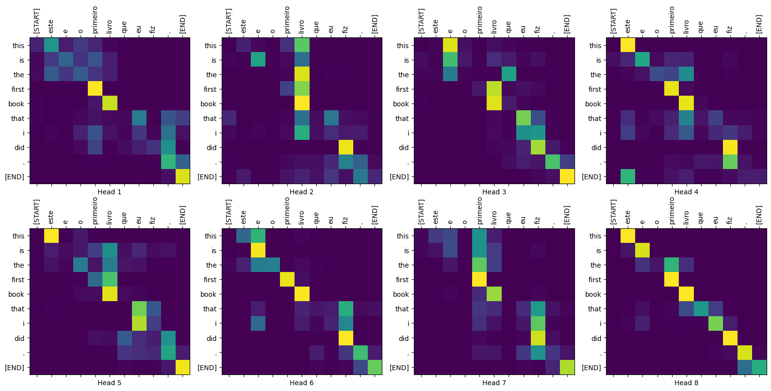
Сюжеты внимания
Класс Translator возвращает словарь карт внимания, которые можно использовать для визуализации внутренней работы модели:
sentence = "este é o primeiro livro que eu fiz."
ground_truth = "this is the first book i've ever done."

translated_text, translated_tokens, attention_weights = translator(
    tf.constant(sentence))
print_translation(sentence, translated_text, ground_truth)
Input:         : este é o primeiro livro que eu fiz.
Prediction     : this is the first book that i did .
Ground truth   : this is the first book i've ever done.
def plot_attention_head(in_tokens, translated_tokens, attention):
  # The plot is of the attention when a token was generated.
  # The model didn't generate `<START>` in the output. Skip it.
  translated_tokens = translated_tokens[1:]

  ax = plt.gca()
  ax.matshow(attention)
  ax.set_xticks(range(len(in_tokens)))
  ax.set_yticks(range(len(translated_tokens)))

  labels = [label.decode('utf-8') for label in in_tokens.numpy()]
  ax.set_xticklabels(
      labels, rotation=90)

  labels = [label.decode('utf-8') for label in translated_tokens.numpy()]
  ax.set_yticklabels(labels)
head = 0
# shape: (batch=1, num_heads, seq_len_q, seq_len_k)
attention_heads = tf.squeeze(
  attention_weights['decoder_layer4_block2'], 0)
attention = attention_heads[head]
attention.shape
TensorShape([10, 11])
in_tokens = tf.convert_to_tensor([sentence])
in_tokens = tokenizers.pt.tokenize(in_tokens).to_tensor()
in_tokens = tokenizers.pt.lookup(in_tokens)[0]
in_tokens
<tf.Tensor: shape=(11,), dtype=string, numpy=
array([b'[START]', b'este', b'e', b'o', b'primeiro', b'livro', b'que',
       b'eu', b'fiz', b'.', b'[END]'], dtype=object)>
translated_tokens
<tf.Tensor: shape=(11,), dtype=string, numpy=
array([b'[START]', b'this', b'is', b'the', b'first', b'book', b'that',
       b'i', b'did', b'.', b'[END]'], dtype=object)>
plot_attention_head(in_tokens, translated_tokens, attention)

def plot_attention_weights(sentence, translated_tokens, attention_heads):
  in_tokens = tf.convert_to_tensor([sentence])
  in_tokens = tokenizers.pt.tokenize(in_tokens).to_tensor()
  in_tokens = tokenizers.pt.lookup(in_tokens)[0]
  in_tokens

  fig = plt.figure(figsize=(16, 8))

  for h, head in enumerate(attention_heads):
    ax = fig.add_subplot(2, 4, h+1)

    plot_attention_head(in_tokens, translated_tokens, head)

    ax.set_xlabel(f'Head {h+1}')

  plt.tight_layout()
  plt.show()
plot_attention_weights(sentence, translated_tokens,
                       attention_weights['decoder_layer4_block2'][0])

Модель хорошо справляется с незнакомыми словами. Во входном наборе данных нет ни «трицератопсов», ни «энциклопедий», и модель почти учится их транслитерировать, даже без общего словаря:
sentence = "Eu li sobre triceratops na enciclopédia."
ground_truth = "I read about triceratops in the encyclopedia."

translated_text, translated_tokens, attention_weights = translator(
    tf.constant(sentence))
print_translation(sentence, translated_text, ground_truth)

plot_attention_weights(sentence, translated_tokens,
                       attention_weights['decoder_layer4_block2'][0])
Input:         : Eu li sobre triceratops na enciclopédia.
Prediction     : i read about trigatotys in the encyclopedia .
Ground truth   : I read about triceratops in the encyclopedia.

Экспорт
Эта модель вывода работает, поэтому теперь вы экспортируете ее как tf.saved_model .
Для этого оберните его еще одним tf.Module , на этот раз с tf.function в методе __call__ :
class ExportTranslator(tf.Module):
  def __init__(self, translator):
    self.translator = translator

  @tf.function(input_signature=[tf.TensorSpec(shape=[], dtype=tf.string)])
  def __call__(self, sentence):
    (result,
     tokens,
     attention_weights) = self.translator(sentence, max_length=100)

    return result
В приведенной выше tf.function только выходное предложение. Благодаря нестрогому исполнению в tf.function никакие ненужные значения никогда не вычисляются.
translator = ExportTranslator(translator)
Поскольку модель декодирует прогнозы с использованием tf.argmax , прогнозы являются детерминированными. Исходная модель и модель, загруженная из SavedModel , должны давать идентичные прогнозы:
translator("este é o primeiro livro que eu fiz.").numpy()
b'this is the first book that i did .'
tf.saved_model.save(translator, export_dir='translator')
2022-02-04 13:19:17.308292: W tensorflow/python/util/util.cc:368] Sets are not currently considered sequences, but this may change in the future, so consider avoiding using them.
WARNING:absl:Found untraced functions such as embedding_4_layer_call_fn, embedding_4_layer_call_and_return_conditional_losses, dropout_37_layer_call_fn, dropout_37_layer_call_and_return_conditional_losses, embedding_5_layer_call_fn while saving (showing 5 of 224). These functions will not be directly callable after loading.
reloaded = tf.saved_model.load('translator')
reloaded("este é o primeiro livro que eu fiz.").numpy()
b'this is the first book that i did .'
Резюме
В этом уроке вы узнали о позиционном кодировании, многоголовом внимании, важности маскирования и о том, как создать трансформер.
Попробуйте использовать другой набор данных для обучения преобразователя. Вы также можете создать базовый преобразователь или преобразователь XL, изменив указанные выше гиперпараметры. Вы также можете использовать слои, определенные здесь, для создания BERT и обучения современных моделей. Кроме того, вы можете реализовать поиск луча, чтобы получить более точные прогнозы.