
| | |  GitHub पर स्रोत देखें GitHub पर स्रोत देखें | |
इस ट्यूटोरियल में शब्द एम्बेडिंग का परिचय है। आप एक भावना वर्गीकरण कार्य के लिए एक साधारण केरस मॉडल का उपयोग करके अपने स्वयं के शब्द एम्बेडिंग को प्रशिक्षित करेंगे, और फिर उन्हें एम्बेडिंग प्रोजेक्टर (नीचे की छवि में दिखाया गया है) में कल्पना करेंगे।

पाठ को संख्याओं के रूप में प्रस्तुत करना
मशीन लर्निंग मॉडल इनपुट के रूप में वैक्टर (संख्याओं की सरणियाँ) लेते हैं। पाठ के साथ काम करते समय, आपको सबसे पहले जो करना चाहिए वह मॉडल को खिलाने से पहले स्ट्रिंग्स को संख्याओं (या पाठ को "वेक्टराइज़" करने के लिए) में बदलने की रणनीति के साथ आता है। इस खंड में, आप ऐसा करने के लिए तीन रणनीतियों को देखेंगे।
एक-गर्म एन्कोडिंग
पहले विचार के रूप में, आप अपनी शब्दावली में प्रत्येक शब्द को "एक-गर्म" एन्कोड कर सकते हैं। "बिल्ली चटाई पर बैठी" वाक्य पर विचार करें। इस वाक्य में शब्दावली (या अद्वितीय शब्द) है (बिल्ली, चटाई, पर, बैठ गया, द)। प्रत्येक शब्द का प्रतिनिधित्व करने के लिए, आप शब्दावली के बराबर लंबाई के साथ एक शून्य वेक्टर बनाएंगे, फिर एक को उस इंडेक्स में रखें जो शब्द से मेल खाता हो। यह दृष्टिकोण निम्नलिखित आरेख में दिखाया गया है।
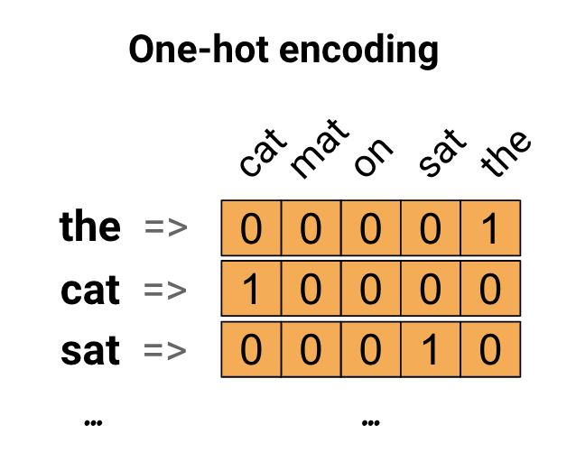
एक वेक्टर बनाने के लिए जिसमें वाक्य की एन्कोडिंग होती है, फिर आप प्रत्येक शब्द के लिए एक-हॉट वैक्टर को जोड़ सकते हैं।
प्रत्येक शब्द को एक अद्वितीय संख्या के साथ एन्कोड करें
एक दूसरा तरीका जो आप आजमा सकते हैं, वह है प्रत्येक शब्द को एक अद्वितीय संख्या का उपयोग करके एन्कोड करना। ऊपर दिए गए उदाहरण को जारी रखते हुए, आप 1 को "बिल्ली", 2 को "चटाई" और इसी तरह असाइन कर सकते हैं। फिर आप वाक्य "बिल्ली चटाई पर बैठी" को घने वेक्टर जैसे [5, 1, 4, 3, 5, 2] के रूप में एन्कोड कर सकते हैं। यह दृष्टिकोण कुशल है। एक विरल वेक्टर के बजाय, अब आपके पास एक घना है (जहां सभी तत्व भरे हुए हैं)।
हालाँकि, इस दृष्टिकोण के दो नुकसान हैं:
पूर्णांक-एन्कोडिंग मनमाना है (यह शब्दों के बीच किसी भी संबंध को कैप्चर नहीं करता है)।
एक मॉडल की व्याख्या करने के लिए एक पूर्णांक-एन्कोडिंग चुनौतीपूर्ण हो सकती है। उदाहरण के लिए, एक लीनियर क्लासिफायरियर प्रत्येक फीचर के लिए सिंगल वेट सीखता है। क्योंकि किन्हीं दो शब्दों की समानता और उनके एन्कोडिंग की समानता के बीच कोई संबंध नहीं है, यह फीचर-वेट संयोजन सार्थक नहीं है।
शब्द एम्बेडिंग
शब्द एम्बेडिंग हमें एक कुशल, सघन प्रतिनिधित्व का उपयोग करने का एक तरीका देता है जिसमें समान शब्दों में समान एन्कोडिंग होती है। महत्वपूर्ण रूप से, आपको इस एन्कोडिंग को हाथ से निर्दिष्ट करने की आवश्यकता नहीं है। एक एम्बेडिंग फ़्लोटिंग पॉइंट मानों का एक घना वेक्टर है (वेक्टर की लंबाई आपके द्वारा निर्दिष्ट पैरामीटर है)। मैन्युअल रूप से एम्बेडिंग के लिए मान निर्दिष्ट करने के बजाय, वे प्रशिक्षण योग्य पैरामीटर हैं (प्रशिक्षण के दौरान मॉडल द्वारा सीखे गए वज़न, उसी तरह एक मॉडल घने परत के लिए वज़न सीखता है)। बड़े डेटासेट के साथ काम करते समय शब्द एम्बेडिंग देखना आम बात है जो 8-आयामी (छोटे डेटासेट के लिए) 1024-आयाम तक हैं। एक उच्च आयामी एम्बेडिंग शब्दों के बीच बढ़िया संबंधों को पकड़ सकता है, लेकिन सीखने के लिए अधिक डेटा लेता है।
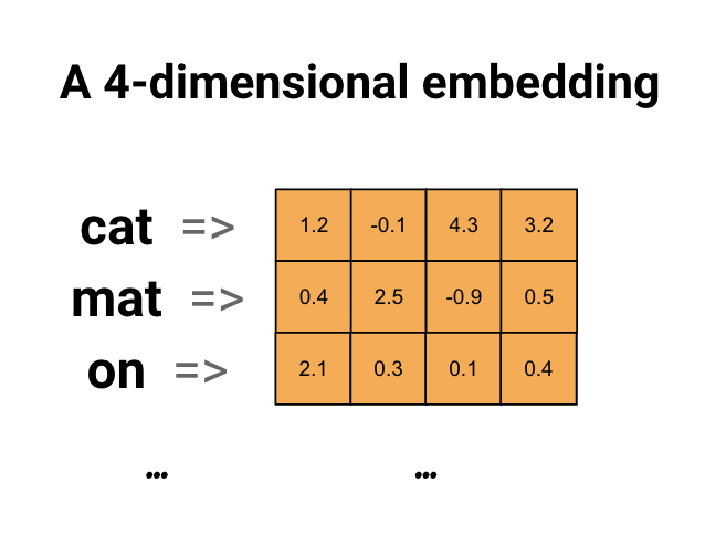
ऊपर एक शब्द एम्बेडिंग के लिए एक आरेख है। प्रत्येक शब्द को फ़्लोटिंग पॉइंट मानों के 4-आयामी वेक्टर के रूप में दर्शाया जाता है। एम्बेडिंग के बारे में सोचने का दूसरा तरीका "लुकअप टेबल" है। इन भारों को सीख लेने के बाद, आप प्रत्येक शब्द को तालिका में संबंधित घने वेक्टर को देखकर एनकोड कर सकते हैं।
सेट अप
import io
import os
import re
import shutil
import string
import tensorflow as tf

from tensorflow.keras import Sequential
from tensorflow.keras.layers import Dense, Embedding, GlobalAveragePooling1D
from tensorflow.keras.layers import TextVectorization
आईएमडीबी डेटासेट डाउनलोड करें
आप ट्यूटोरियल के माध्यम से लार्ज मूवी रिव्यू डेटासेट का उपयोग करेंगे। आप इस डेटासेट पर एक सेंटीमेंट क्लासिफायर मॉडल को प्रशिक्षित करेंगे और इस प्रक्रिया में स्क्रैच से एम्बेडिंग सीखेंगे। किसी डेटासेट को शुरू से लोड करने के बारे में अधिक पढ़ने के लिए, लोड हो रहा टेक्स्ट ट्यूटोरियल देखें।
केरस फ़ाइल उपयोगिता का उपयोग करके डेटासेट डाउनलोड करें और निर्देशिकाओं पर एक नज़र डालें।
url = "https://ai.stanford.edu/~amaas/data/sentiment/aclImdb_v1.tar.gz"

dataset = tf.keras.utils.get_file("aclImdb_v1.tar.gz", url,
                                  untar=True, cache_dir='.',
                                  cache_subdir='')

dataset_dir = os.path.join(os.path.dirname(dataset), 'aclImdb')
os.listdir(dataset_dir)
Downloading data from https://ai.stanford.edu/~amaas/data/sentiment/aclImdb_v1.tar.gz
84131840/84125825 [==============================] - 7s 0us/step
84140032/84125825 [==============================] - 7s 0us/step
['test', 'imdb.vocab', 'imdbEr.txt', 'train', 'README']
train/ निर्देशिका पर एक नज़र डालें। इसमें सकारात्मक और नकारात्मक के रूप में लेबल की गई मूवी समीक्षाओं के साथ pos और neg फ़ोल्डर हैं। बाइनरी वर्गीकरण मॉडल को प्रशिक्षित करने के लिए आप pos और neg फ़ोल्डरों की समीक्षाओं का उपयोग करेंगे।
train_dir = os.path.join(dataset_dir, 'train')
os.listdir(train_dir)
['urls_pos.txt',
 'urls_unsup.txt',
 'urls_neg.txt',
 'pos',
 'unsup',
 'unsupBow.feat',
 'neg',
 'labeledBow.feat']
train निर्देशिका में अतिरिक्त फ़ोल्डर भी होते हैं जिन्हें प्रशिक्षण डेटासेट बनाने से पहले हटा दिया जाना चाहिए।
remove_dir = os.path.join(train_dir, 'unsup')
shutil.rmtree(remove_dir)
इसके बाद, tf.keras.utils.text_dataset_from_directory का उपयोग करके एक tf.data.Dataset tf.keras.utils.text_dataset_from_directory । आप इस उपयोगिता का उपयोग करने के बारे में इस पाठ वर्गीकरण ट्यूटोरियल में अधिक पढ़ सकते हैं।
सत्यापन के लिए 20% के विभाजन के साथ ट्रेन और सत्यापन डेटासेट दोनों बनाने के लिए train निर्देशिका का उपयोग करें।
batch_size = 1024
seed = 123
train_ds = tf.keras.utils.text_dataset_from_directory(
    'aclImdb/train', batch_size=batch_size, validation_split=0.2,
    subset='training', seed=seed)
val_ds = tf.keras.utils.text_dataset_from_directory(
    'aclImdb/train', batch_size=batch_size, validation_split=0.2,
    subset='validation', seed=seed)
Found 25000 files belonging to 2 classes.
Using 20000 files for training.
Found 25000 files belonging to 2 classes.
Using 5000 files for validation.
ट्रेन डेटासेट से कुछ मूवी समीक्षाओं और उनके लेबल (1: positive, 0: negative) पर एक नज़र डालें।
for text_batch, label_batch in train_ds.take(1):
  for i in range(5):
    print(label_batch[i].numpy(), text_batch.numpy()[i])
0 b"Oh My God! Please, for the love of all that is holy, Do Not Watch This Movie! It it 82 minutes of my life I will never get back. Sure, I could have stopped watching half way through. But I thought it might get better. It Didn't. Anyone who actually enjoyed this movie is one seriously sick and twisted individual. No wonder us Australians/New Zealanders have a terrible reputation when it comes to making movies. Everything about this movie is horrible, from the acting to the editing. I don't even normally write reviews on here, but in this case I'll make an exception. I only wish someone had of warned me before I hired this catastrophe"
1 b'This movie is SOOOO funny!!! The acting is WONDERFUL, the Ramones are sexy, the jokes are subtle, and the plot is just what every high schooler dreams of doing to his/her school. I absolutely loved the soundtrack as well as the carefully placed cynicism. If you like monty python, You will love this film. This movie is a tad bit "grease"esk (without all the annoying songs). The songs that are sung are likable; you might even find yourself singing these songs once the movie is through. This musical ranks number two in musicals to me (second next to the blues brothers). But please, do not think of it as a musical per say; seeing as how the songs are so likable, it is hard to tell a carefully choreographed scene is taking place. I think of this movie as more of a comedy with undertones of romance. You will be reminded of what it was like to be a rebellious teenager; needless to say, you will be reminiscing of your old high school days after seeing this film. Highly recommended for both the family (since it is a very youthful but also for adults since there are many jokes that are funnier with age and experience.'
0 b"Alex D. Linz replaces Macaulay Culkin as the central figure in the third movie in the Home Alone empire. Four industrial spies acquire a missile guidance system computer chip and smuggle it through an airport inside a remote controlled toy car. Because of baggage confusion, grouchy Mrs. Hess (Marian Seldes) gets the car. She gives it to her neighbor, Alex (Linz), just before the spies turn up. The spies rent a house in order to burglarize each house in the neighborhood until they locate the car. Home alone with the chicken pox, Alex calls 911 each time he spots a theft in progress, but the spies always manage to elude the police while Alex is accused of making prank calls. The spies finally turn their attentions toward Alex, unaware that he has rigged devices to cleverly booby-trap his entire house. Home Alone 3 wasn't horrible, but probably shouldn't have been made, you can't just replace Macauley Culkin, Joe Pesci, or Daniel Stern. Home Alone 3 had some funny parts, but I don't like when characters are changed in a movie series, view at own risk."
0 b"There's a good movie lurking here, but this isn't it. The basic idea is good: to explore the moral issues that would face a group of young survivors of the apocalypse. But the logic is so muddled that it's impossible to get involved.<br /><br />For example, our four heroes are (understandably) paranoid about catching the mysterious airborne contagion that's wiped out virtually all of mankind. Yet they wear surgical masks some times, not others. Some times they're fanatical about wiping down with bleach any area touched by an infected person. Other times, they seem completely unconcerned.<br /><br />Worse, after apparently surviving some weeks or months in this new kill-or-be-killed world, these people constantly behave like total newbs. They don't bother accumulating proper equipment, or food. They're forever running out of fuel in the middle of nowhere. They don't take elementary precautions when meeting strangers. And after wading through the rotting corpses of the entire human race, they're as squeamish as sheltered debutantes. You have to constantly wonder how they could have survived this long... and even if they did, why anyone would want to make a movie about them.<br /><br />So when these dweebs stop to agonize over the moral dimensions of their actions, it's impossible to take their soul-searching seriously. Their actions would first have to make some kind of minimal sense.<br /><br />On top of all this, we must contend with the dubious acting abilities of Chris Pine. His portrayal of an arrogant young James T Kirk might have seemed shrewd, when viewed in isolation. But in Carriers he plays on exactly that same note: arrogant and boneheaded. It's impossible not to suspect that this constitutes his entire dramatic range.<br /><br />On the positive side, the film *looks* excellent. It's got an over-sharp, saturated look that really suits the southwestern US locale. But that can't save the truly feeble writing nor the paper-thin (and annoying) characters. Even if you're a fan of the end-of-the-world genre, you should save yourself the agony of watching Carriers."
0 b'I saw this movie at an actual movie theater (probably the \\(2.00 one) with my cousin and uncle. We were around 11 and 12, I guess, and really into scary movies. I remember being so excited to see it because my cool uncle let us pick the movie (and we probably never got to do that again!) and sooo disappointed afterwards!! Just boring and not scary. The only redeeming thing I can remember was Corky Pigeon from Silver Spoons, and that wasn\'t all that great, just someone I recognized. I\'ve seen bad movies before and this one has always stuck out in my mind as the worst. This was from what I can recall, one of the most boring, non-scary, waste of our collective \\)6, and a waste of film. I have read some of the reviews that say it is worth a watch and I say, "Too each his own", but I wouldn\'t even bother. Not even so bad it\'s good.'
प्रदर्शन के लिए डेटासेट कॉन्फ़िगर करें
ये दो महत्वपूर्ण तरीके हैं जिनका उपयोग आपको डेटा लोड करते समय यह सुनिश्चित करने के लिए करना चाहिए कि I/O अवरुद्ध न हो जाए।
.cache() डिस्क से लोड होने के बाद डेटा को मेमोरी में रखता है। यह सुनिश्चित करेगा कि आपके मॉडल को प्रशिक्षित करते समय डेटासेट एक अड़चन न बने। यदि आपका डेटासेट मेमोरी में फ़िट होने के लिए बहुत बड़ा है, तो आप इस पद्धति का उपयोग एक प्रदर्शनकारी ऑन-डिस्क कैश बनाने के लिए भी कर सकते हैं, जो कई छोटी फ़ाइलों की तुलना में पढ़ने में अधिक कुशल है।
.prefetch() प्रशिक्षण के दौरान डेटा प्रीप्रोसेसिंग और मॉडल निष्पादन को ओवरलैप करता है।
आप दोनों विधियों के साथ-साथ डेटा प्रदर्शन मार्गदर्शिका में डिस्क पर डेटा कैश करने के तरीके के बारे में अधिक जान सकते हैं।
AUTOTUNE = tf.data.AUTOTUNE

train_ds = train_ds.cache().prefetch(buffer_size=AUTOTUNE)
val_ds = val_ds.cache().prefetch(buffer_size=AUTOTUNE)
एम्बेडिंग परत का उपयोग करना
केरस शब्द एम्बेडिंग का उपयोग करना आसान बनाता है। एम्बेडिंग परत पर एक नज़र डालें।
एम्बेडिंग परत को एक लुकअप तालिका के रूप में समझा जा सकता है जो पूर्णांक सूचकांक (जो विशिष्ट शब्दों के लिए खड़ा है) से घने वैक्टर (उनकी एम्बेडिंग) तक मैप करता है। एम्बेडिंग की आयामीता (या चौड़ाई) एक पैरामीटर है जिसके साथ आप यह देखने के लिए प्रयोग कर सकते हैं कि आपकी समस्या के लिए क्या अच्छा काम करता है, ठीक उसी तरह जैसे आप घने परत में न्यूरॉन्स की संख्या के साथ प्रयोग करेंगे।
# Embed a 1,000 word vocabulary into 5 dimensions.
embedding_layer = tf.keras.layers.Embedding(1000, 5)
जब आप एक एम्बेडिंग परत बनाते हैं, तो एम्बेडिंग के लिए वज़न बेतरतीब ढंग से आरंभ किया जाता है (किसी भी अन्य परत की तरह)। प्रशिक्षण के दौरान, उन्हें धीरे-धीरे बैकप्रोपेगेशन के माध्यम से समायोजित किया जाता है। एक बार प्रशिक्षित होने के बाद, सीखे गए शब्द एम्बेडिंग शब्दों के बीच समानता को मोटे तौर पर सांकेतिक शब्दों में बदल देंगे (जैसा कि वे उस विशिष्ट समस्या के लिए सीखे गए थे जिस पर आपका मॉडल प्रशिक्षित है)।
यदि आप एक पूर्णांक को एक एम्बेडिंग परत में पास करते हैं, तो परिणाम प्रत्येक पूर्णांक को एम्बेडिंग तालिका से वेक्टर के साथ बदल देता है:
result = embedding_layer(tf.constant([1, 2, 3]))
result.numpy()
array([[ 0.01318491, -0.02219239,  0.024673  , -0.03208025,  0.02297195],
       [-0.00726584,  0.03731754, -0.01209557, -0.03887399, -0.02407478],
       [ 0.04477594,  0.04504738, -0.02220147, -0.03642888, -0.04688282]],
      dtype=float32)
पाठ या अनुक्रम की समस्याओं के लिए, एम्बेडिंग परत आकार (samples, sequence_length) के पूर्णांकों का एक 2D टेंसर लेती है, जहां प्रत्येक प्रविष्टि पूर्णांकों का एक क्रम है। यह परिवर्तनीय लंबाई के अनुक्रम एम्बेड कर सकता है। आप आकार (32, 10) (लंबाई 10 के 32 अनुक्रमों का बैच) या (64, 15) (लंबाई 15 के 64 अनुक्रमों का बैच) के साथ बैचों के ऊपर एम्बेडिंग परत में फ़ीड कर सकते हैं।
लौटाए गए टेंसर में इनपुट की तुलना में एक और अक्ष होता है, एम्बेडिंग वैक्टर नए अंतिम अक्ष के साथ संरेखित होते हैं। इसे एक (2, 3) इनपुट बैच पास करें और आउटपुट (2, 3, N)
result = embedding_layer(tf.constant([[0, 1, 2], [3, 4, 5]]))
result.shape
TensorShape([2, 3, 5])प्लेसहोल्डर17
जब इनपुट के रूप में अनुक्रमों का एक बैच दिया जाता है, तो एक एम्बेडिंग परत आकार (samples, sequence_length, embedding_dimensionality) का एक 3D फ़्लोटिंग पॉइंट टेंसर देता है। परिवर्तनीय लंबाई के इस अनुक्रम से एक निश्चित प्रतिनिधित्व में परिवर्तित करने के लिए कई प्रकार के मानक दृष्टिकोण हैं। आप RNN, अटेंशन या पूलिंग लेयर को Dense लेयर में भेजने से पहले उपयोग कर सकते हैं। यह ट्यूटोरियल पूलिंग का उपयोग करता है क्योंकि यह सबसे सरल है। आरएनएन ट्यूटोरियल के साथ टेक्स्ट क्लासिफिकेशन एक अच्छा अगला कदम है।
टेक्स्ट प्रीप्रोसेसिंग
इसके बाद, अपने सेंटीमेंट वर्गीकरण मॉडल के लिए आवश्यक डेटासेट प्रीप्रोसेसिंग चरणों को परिभाषित करें। मूवी समीक्षाओं को वेक्टराइज़ करने के लिए वांछित पैरामीटर के साथ टेक्स्ट वेक्टराइज़ेशन परत प्रारंभ करें। आप पाठ वर्गीकरण ट्यूटोरियल में इस परत का उपयोग करने के बारे में अधिक जान सकते हैं।
# Create a custom standardization function to strip HTML break tags '<br />'.
def custom_standardization(input_data):
  lowercase = tf.strings.lower(input_data)
  stripped_html = tf.strings.regex_replace(lowercase, '<br />', ' ')
  return tf.strings.regex_replace(stripped_html,
                                  '[%s]' % re.escape(string.punctuation), '')


# Vocabulary size and number of words in a sequence.
vocab_size = 10000
sequence_length = 100

# Use the text vectorization layer to normalize, split, and map strings to
# integers. Note that the layer uses the custom standardization defined above.
# Set maximum_sequence length as all samples are not of the same length.
vectorize_layer = TextVectorization(
    standardize=custom_standardization,
    max_tokens=vocab_size,
    output_mode='int',
    output_sequence_length=sequence_length)

# Make a text-only dataset (no labels) and call adapt to build the vocabulary.
text_ds = train_ds.map(lambda x, y: x)
vectorize_layer.adapt(text_ds)
एक वर्गीकरण मॉडल बनाएं
भावना वर्गीकरण मॉडल को परिभाषित करने के लिए केरस अनुक्रमिक एपीआई का प्रयोग करें। इस मामले में यह "शब्दों का सतत बैग" शैली मॉडल है।
-
TextVectorizationलेयर स्ट्रिंग्स को शब्दावली सूचकांकों में बदल देती है। आपने पहले हीvectorize_layerको TextVectorization लेयर के रूप में प्रारंभ कर दिया है औरadaptपरtext_dsको कॉल करके इसकी शब्दावली का निर्माण किया है। अब vectorize_layer का उपयोग आपके एंड-टू-एंड वर्गीकरण मॉडल की पहली परत के रूप में किया जा सकता है, जो रूपांतरित स्ट्रिंग्स को एम्बेडिंग परत में फीड करता है। Embeddingपरत पूर्णांक-एन्कोडेड शब्दावली लेती है और प्रत्येक शब्द-अनुक्रमणिका के लिए एम्बेडिंग वेक्टर को देखती है। इन वैक्टर को मॉडल ट्रेन के रूप में सीखा जाता है। वेक्टर आउटपुट सरणी में एक आयाम जोड़ते हैं। परिणामी आयाम हैं:(batch, sequence, embedding)।GlobalAveragePooling1Dपरत प्रत्येक उदाहरण के लिए अनुक्रम आयाम पर औसत द्वारा एक निश्चित-लंबाई आउटपुट वेक्टर देता है। यह मॉडल को यथासंभव सरलतम तरीके से परिवर्तनीय लंबाई के इनपुट को संभालने की अनुमति देता है।फिक्स्ड-लेंथ आउटपुट वेक्टर को 16 छिपी इकाइयों के साथ पूरी तरह से कनेक्टेड (
Dense) परत के माध्यम से पाइप किया जाता है।अंतिम परत एकल आउटपुट नोड के साथ घनी रूप से जुड़ी हुई है।
embedding_dim=16

model = Sequential([
  vectorize_layer,
  Embedding(vocab_size, embedding_dim, name="embedding"),
  GlobalAveragePooling1D(),
  Dense(16, activation='relu'),
  Dense(1)
])
मॉडल को संकलित और प्रशिक्षित करें
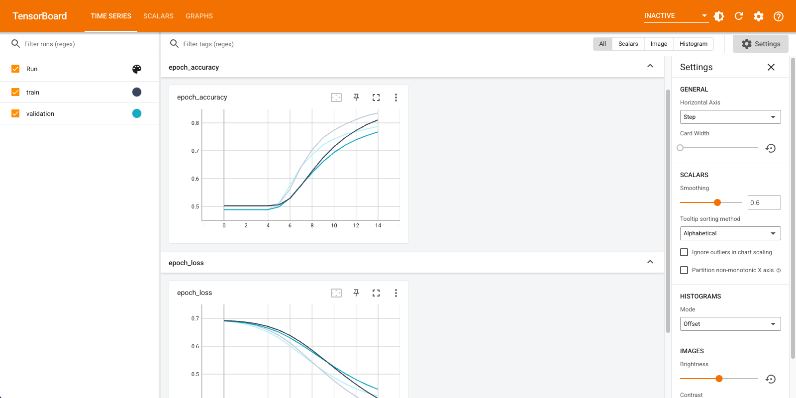
नुकसान और सटीकता सहित मीट्रिक की कल्पना करने के लिए आप TensorBoard का उपयोग करेंगे। एक tf.keras.callbacks.TensorBoard बनाएँ।
tensorboard_callback = tf.keras.callbacks.TensorBoard(log_dir="logs")
Adam ऑप्टिमाइज़र और BinaryCrossentropy लॉस का उपयोग करके मॉडल को संकलित और प्रशिक्षित करें।
model.compile(optimizer='adam',
              loss=tf.keras.losses.BinaryCrossentropy(from_logits=True),
              metrics=['accuracy'])
model.fit(
    train_ds,
    validation_data=val_ds,
    epochs=15,
    callbacks=[tensorboard_callback])
Epoch 1/15
20/20 [==============================] - 2s 71ms/step - loss: 0.6910 - accuracy: 0.5028 - val_loss: 0.6878 - val_accuracy: 0.4886
Epoch 2/15
20/20 [==============================] - 1s 57ms/step - loss: 0.6838 - accuracy: 0.5028 - val_loss: 0.6791 - val_accuracy: 0.4886
Epoch 3/15
20/20 [==============================] - 1s 58ms/step - loss: 0.6726 - accuracy: 0.5028 - val_loss: 0.6661 - val_accuracy: 0.4886
Epoch 4/15
20/20 [==============================] - 1s 58ms/step - loss: 0.6563 - accuracy: 0.5028 - val_loss: 0.6481 - val_accuracy: 0.4886
Epoch 5/15
20/20 [==============================] - 1s 58ms/step - loss: 0.6343 - accuracy: 0.5061 - val_loss: 0.6251 - val_accuracy: 0.5066
Epoch 6/15
20/20 [==============================] - 1s 58ms/step - loss: 0.6068 - accuracy: 0.5634 - val_loss: 0.5982 - val_accuracy: 0.5762
Epoch 7/15
20/20 [==============================] - 1s 58ms/step - loss: 0.5752 - accuracy: 0.6405 - val_loss: 0.5690 - val_accuracy: 0.6386
Epoch 8/15
20/20 [==============================] - 1s 58ms/step - loss: 0.5412 - accuracy: 0.7036 - val_loss: 0.5390 - val_accuracy: 0.6850
Epoch 9/15
20/20 [==============================] - 1s 59ms/step - loss: 0.5064 - accuracy: 0.7479 - val_loss: 0.5106 - val_accuracy: 0.7222
Epoch 10/15
20/20 [==============================] - 1s 59ms/step - loss: 0.4734 - accuracy: 0.7774 - val_loss: 0.4855 - val_accuracy: 0.7430
Epoch 11/15
20/20 [==============================] - 1s 59ms/step - loss: 0.4432 - accuracy: 0.7971 - val_loss: 0.4636 - val_accuracy: 0.7570
Epoch 12/15
20/20 [==============================] - 1s 58ms/step - loss: 0.4161 - accuracy: 0.8155 - val_loss: 0.4453 - val_accuracy: 0.7674
Epoch 13/15
20/20 [==============================] - 1s 59ms/step - loss: 0.3921 - accuracy: 0.8304 - val_loss: 0.4303 - val_accuracy: 0.7780
Epoch 14/15
20/20 [==============================] - 1s 61ms/step - loss: 0.3711 - accuracy: 0.8398 - val_loss: 0.4181 - val_accuracy: 0.7884
Epoch 15/15
20/20 [==============================] - 1s 58ms/step - loss: 0.3524 - accuracy: 0.8493 - val_loss: 0.4082 - val_accuracy: 0.7948
<keras.callbacks.History at 0x7fca579745d0>
इस दृष्टिकोण के साथ मॉडल लगभग 78% की सत्यापन सटीकता तक पहुंचता है (ध्यान दें कि मॉडल अधिक उपयुक्त है क्योंकि प्रशिक्षण सटीकता अधिक है)।
आप मॉडल की प्रत्येक परत के बारे में अधिक जानने के लिए मॉडल सारांश देख सकते हैं।
model.summary()
Model: "sequential"
_________________________________________________________________
 Layer (type)                Output Shape              Param #
=================================================================
 text_vectorization (TextVec  (None, 100)              0
 torization)

 embedding (Embedding)       (None, 100, 16)           160000

 global_average_pooling1d (G  (None, 16)               0
 lobalAveragePooling1D)

 dense (Dense)               (None, 16)                272

 dense_1 (Dense)             (None, 1)                 17

=================================================================
Total params: 160,289
Trainable params: 160,289
Non-trainable params: 0
_________________________________________________________________
TensorBoard में मॉडल मेट्रिक्स की कल्पना करें।
#docs_infra: no_execute
%load_ext tensorboard
%tensorboard --logdir logs
प्रशिक्षित शब्द एम्बेडिंग को पुनः प्राप्त करें और उन्हें डिस्क पर सहेजें
इसके बाद, प्रशिक्षण के दौरान सीखे गए शब्द एम्बेडिंग को पुनः प्राप्त करें। एम्बेडिंग मॉडल में एंबेडिंग परत के भार हैं। वज़न मैट्रिक्स आकार का है (vocab_size, embedding_dimension) ।
get_layer() और get_weights() ) का उपयोग करके मॉडल से वज़न प्राप्त करें। get_vocabulary() फ़ंक्शन प्रति पंक्ति एक टोकन के साथ मेटाडेटा फ़ाइल बनाने के लिए शब्दावली प्रदान करता है।
weights = model.get_layer('embedding').get_weights()[0]
vocab = vectorize_layer.get_vocabulary()
डिस्क पर भार लिखें। एम्बेडिंग प्रोजेक्टर का उपयोग करने के लिए, आप टैब से अलग किए गए प्रारूप में दो फ़ाइलें अपलोड करेंगे: वैक्टर की एक फ़ाइल (एम्बेडिंग युक्त), और मेटा डेटा की एक फ़ाइल (शब्दों से युक्त)।
out_v = io.open('vectors.tsv', 'w', encoding='utf-8')
out_m = io.open('metadata.tsv', 'w', encoding='utf-8')

for index, word in enumerate(vocab):
  if index == 0:
    continue  # skip 0, it's padding.
  vec = weights[index]
  out_v.write('\t'.join([str(x) for x in vec]) + "\n")
  out_m.write(word + "\n")
out_v.close()
out_m.close()
यदि आप इस ट्यूटोरियल को Colaboratory में चला रहे हैं, तो आप इन फ़ाइलों को अपनी स्थानीय मशीन पर डाउनलोड करने के लिए निम्न स्निपेट का उपयोग कर सकते हैं (या फ़ाइल ब्राउज़र का उपयोग करें, देखें -> सामग्री तालिका -> फ़ाइल ब्राउज़र )।
try:
  from google.colab import files
  files.download('vectors.tsv')
  files.download('metadata.tsv')
except Exception:
  pass
एम्बेडिंग की कल्पना करें
एम्बेडिंग की कल्पना करने के लिए, उन्हें एम्बेडिंग प्रोजेक्टर पर अपलोड करें।
एम्बेडिंग प्रोजेक्टर खोलें (यह स्थानीय TensorBoard उदाहरण में भी चल सकता है)।
"डेटा लोड करें" पर क्लिक करें।
आपके द्वारा ऊपर बनाई गई दो फ़ाइलें अपलोड करें:
vecs.tsvऔरmeta.tsv।
आपके द्वारा प्रशिक्षित किए गए एम्बेडिंग अब प्रदर्शित होंगे। आप उनके निकटतम पड़ोसियों को खोजने के लिए शब्दों की खोज कर सकते हैं। उदाहरण के लिए, "सुंदर" खोजने का प्रयास करें। आप पड़ोसियों को "अद्भुत" जैसे देख सकते हैं।
अगले कदम
इस ट्यूटोरियल ने आपको दिखाया है कि कैसे एक छोटे डेटासेट पर शब्द एम्बेडिंग को शुरू से ही प्रशिक्षित और विज़ुअलाइज़ किया जाए।
Word2Vec एल्गोरिथम का उपयोग करके शब्द एम्बेडिंग को प्रशिक्षित करने के लिए, Word2Vec ट्यूटोरियल आज़माएं।
उन्नत टेक्स्ट प्रोसेसिंग के बारे में अधिक जानने के लिए, भाषा समझने के लिए ट्रांसफॉर्मर मॉडल पढ़ें।