
Copyright 2023 The TF-Agents Authors.
|
|
|
 View source on GitHub
|
|
Introduction
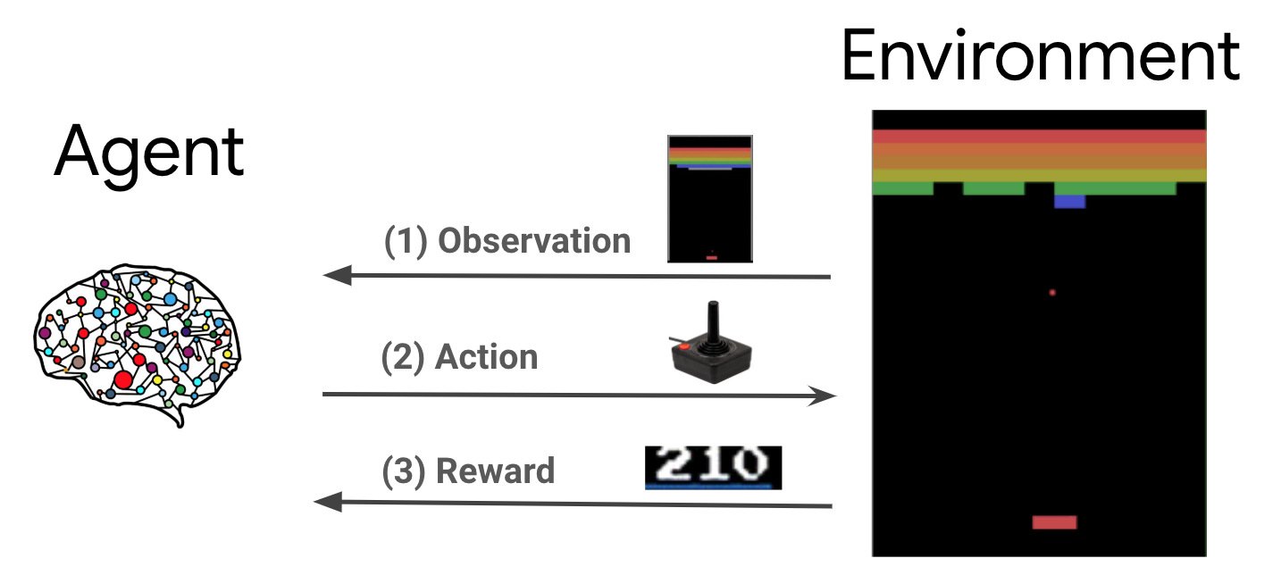
Reinforcement learning (RL) is a general framework where agents learn to perform actions in an environment so as to maximize a reward. The two main components are the environment, which represents the problem to be solved, and the agent, which represents the learning algorithm.
The agent and environment continuously interact with each other. At each time step, the agent takes an action on the environment based on its policy \(\pi(a_t|s_t)\), where \(s_t\) is the current observation from the environment, and receives a reward \(r_{t+1}\) and the next observation \(s_{t+1}\) from the environment. The goal is to improve the policy so as to maximize the sum of rewards (return).
This is a very general framework and can model a variety of sequential decision making problems such as games, robotics etc.
The Cartpole Environment
The Cartpole environment is one of the most well known classic reinforcement learning problems ( the "Hello, World!" of RL). A pole is attached to a cart, which can move along a frictionless track. The pole starts upright and the goal is to prevent it from falling over by controlling the cart.
- The observation from the environment \(s_t\) is a 4D vector representing the position and velocity of the cart, and the angle and angular velocity of the pole.
- The agent can control the system by taking one of 2 actions \(a_t\): push the cart right (+1) or left (-1).
- A reward \(r_{t+1} = 1\) is provided for every timestep that the pole remains upright. The episode ends when one of the following is true:
- the pole tips over some angle limit
- the cart moves outside of the world edges
- 200 time steps pass.
The goal of the agent is to learn a policy \(\pi(a_t|s_t)\) so as to maximize the sum of rewards in an episode \(\sum_{t=0}^{T} \gamma^t r_t\). Here \(\gamma\) is a discount factor in \([0, 1]\) that discounts future rewards relative to immediate rewards. This parameter helps us focus the policy, making it care more about obtaining rewards quickly.
The DQN Agent
The DQN (Deep Q-Network) algorithm was developed by DeepMind in 2015. It was able to solve a wide range of Atari games (some to superhuman level) by combining reinforcement learning and deep neural networks at scale. The algorithm was developed by enhancing a classic RL algorithm called Q-Learning with deep neural networks and a technique called experience replay.
Q-Learning
Q-Learning is based on the notion of a Q-function. The Q-function (a.k.a the state-action value function) of a policy \(\pi\), \(Q^{\pi}(s, a)\), measures the expected return or discounted sum of rewards obtained from state \(s\) by taking action \(a\) first and following policy \(\pi\) thereafter. We define the optimal Q-function \(Q^*(s, a)\) as the maximum return that can be obtained starting from observation \(s\), taking action \(a\) and following the optimal policy thereafter. The optimal Q-function obeys the following Bellman optimality equation:
\(\begin{equation}Q^\ast(s, a) = \mathbb{E}[ r + \gamma \max_{a'} Q^\ast(s', a') ]\end{equation}\)
This means that the maximum return from state \(s\) and action \(a\) is the sum of the immediate reward \(r\) and the return (discounted by \(\gamma\)) obtained by following the optimal policy thereafter until the end of the episode (i.e., the maximum reward from the next state \(s'\)). The expectation is computed both over the distribution of immediate rewards \(r\) and possible next states \(s'\).
The basic idea behind Q-Learning is to use the Bellman optimality equation as an iterative update \(Q_{i+1}(s, a) \leftarrow \mathbb{E}\left[ r + \gamma \max_{a'} Q_{i}(s', a')\right]\), and it can be shown that this converges to the optimal \(Q\)-function, i.e. \(Q_i \rightarrow Q^*\) as \(i \rightarrow \infty\) (see the DQN paper).
Deep Q-Learning
For most problems, it is impractical to represent the \(Q\)-function as a table containing values for each combination of \(s\) and \(a\). Instead, we train a function approximator, such as a neural network with parameters \(\theta\), to estimate the Q-values, i.e. \(Q(s, a; \theta) \approx Q^*(s, a)\). This can done by minimizing the following loss at each step \(i\):
\(\begin{equation}L_i(\theta_i) = \mathbb{E}_{s, a, r, s'\sim \rho(.)} \left[ (y_i - Q(s, a; \theta_i))^2 \right]\end{equation}\) where \(y_i = r + \gamma \max_{a'} Q(s', a'; \theta_{i-1})\)
Here, \(y_i\) is called the TD (temporal difference) target, and \(y_i - Q\) is called the TD error. \(\rho\) represents the behaviour distribution, the distribution over transitions \(\{s, a, r, s'\}\) collected from the environment.
Note that the parameters from the previous iteration \(\theta_{i-1}\) are fixed and not updated. In practice we use a snapshot of the network parameters from a few iterations ago instead of the last iteration. This copy is called the target network.
Q-Learning is an off-policy algorithm that learns about the greedy policy \(a = \max_{a} Q(s, a; \theta)\) while using a different behaviour policy for acting in the environment/collecting data. This behaviour policy is usually an \(\epsilon\)-greedy policy that selects the greedy action with probability \(1-\epsilon\) and a random action with probability \(\epsilon\) to ensure good coverage of the state-action space.
Experience Replay
To avoid computing the full expectation in the DQN loss, we can minimize it using stochastic gradient descent. If the loss is computed using just the last transition \(\{s, a, r, s'\}\), this reduces to standard Q-Learning.
The Atari DQN work introduced a technique called Experience Replay to make the network updates more stable. At each time step of data collection, the transitions are added to a circular buffer called the replay buffer. Then during training, instead of using just the latest transition to compute the loss and its gradient, we compute them using a mini-batch of transitions sampled from the replay buffer. This has two advantages: better data efficiency by reusing each transition in many updates, and better stability using uncorrelated transitions in a batch.
DQN on Cartpole in TF-Agents
TF-Agents provides all the components necessary to train a DQN agent, such as the agent itself, the environment, policies, networks, replay buffers, data collection loops, and metrics. These components are implemented as Python functions or TensorFlow graph ops, and we also have wrappers for converting between them. Additionally, TF-Agents supports TensorFlow 2.0 mode, which enables us to use TF in imperative mode.
Next, take a look at the tutorial for training a DQN agent on the Cartpole environment using TF-Agents.