
|
|
|
 View source on GitHub View source on GitHub
|
|
When building machine learning models, you need to choose various hyperparameters, such as the dropout rate in a layer or the learning rate. These decisions impact model metrics, such as accuracy. Therefore, an important step in the machine learning workflow is to identify the best hyperparameters for your problem, which often involves experimentation. This process is known as "Hyperparameter Optimization" or "Hyperparameter Tuning".
The HParams dashboard in TensorBoard provides several tools to help with this process of identifying the best experiment or most promising sets of hyperparameters.
This tutorial will focus on the following steps:
- Experiment setup and HParams summary
- Adapt TensorFlow runs to log hyperparameters and metrics
- Start runs and log them all under one parent directory
- Visualize the results in TensorBoard's HParams dashboard
Start by installing TF 2.0 and loading the TensorBoard notebook extension:
# Load the TensorBoard notebook extension
%load_ext tensorboard
# Clear any logs from previous runsrm -rf ./logs/
Import TensorFlow and the TensorBoard HParams plugin:
import tensorflow as tf
from tensorboard.plugins.hparams import api as hp
Download the FashionMNIST dataset and scale it:
fashion_mnist = tf.keras.datasets.fashion_mnist

(x_train, y_train),(x_test, y_test) = fashion_mnist.load_data()
x_train, x_test = x_train / 255.0, x_test / 255.0
Downloading data from https://storage.googleapis.com/tensorflow/tf-keras-datasets/train-labels-idx1-ubyte.gz
32768/29515 [=================================] - 0s 0us/step
Downloading data from https://storage.googleapis.com/tensorflow/tf-keras-datasets/train-images-idx3-ubyte.gz
26427392/26421880 [==============================] - 0s 0us/step
Downloading data from https://storage.googleapis.com/tensorflow/tf-keras-datasets/t10k-labels-idx1-ubyte.gz
8192/5148 [===============================================] - 0s 0us/step
Downloading data from https://storage.googleapis.com/tensorflow/tf-keras-datasets/t10k-images-idx3-ubyte.gz
4423680/4422102 [==============================] - 0s 0us/step
1. Experiment setup and the HParams experiment summary
Experiment with three hyperparameters in the model:
- Number of units in the first dense layer
- Dropout rate in the dropout layer
- Optimizer
List the values to try, and log an experiment configuration to TensorBoard. This step is optional: you can provide domain information to enable more precise filtering of hyperparameters in the UI, and you can specify which metrics should be displayed.
HP_NUM_UNITS = hp.HParam('num_units', hp.Discrete([16, 32]))
HP_DROPOUT = hp.HParam('dropout', hp.RealInterval(0.1, 0.2))
HP_OPTIMIZER = hp.HParam('optimizer', hp.Discrete(['adam', 'sgd']))

METRIC_ACCURACY = 'accuracy'

with tf.summary.create_file_writer('logs/hparam_tuning').as_default():
  hp.hparams_config(
    hparams=[HP_NUM_UNITS, HP_DROPOUT, HP_OPTIMIZER],
    metrics=[hp.Metric(METRIC_ACCURACY, display_name='Accuracy')],
  )
If you choose to skip this step, you can use a string literal wherever you would otherwise use an HParam value: e.g., hparams['dropout'] instead of hparams[HP_DROPOUT].
2. Adapt TensorFlow runs to log hyperparameters and metrics
The model will be quite simple: two dense layers with a dropout layer between them. The training code will look familiar, although the hyperparameters are no longer hardcoded. Instead, the hyperparameters are provided in an hparams dictionary and used throughout the training function:
def train_test_model(hparams):
  model = tf.keras.models.Sequential([
    tf.keras.layers.Flatten(),
    tf.keras.layers.Dense(hparams[HP_NUM_UNITS], activation=tf.nn.relu),
    tf.keras.layers.Dropout(hparams[HP_DROPOUT]),
    tf.keras.layers.Dense(10, activation=tf.nn.softmax),
  ])
  model.compile(
      optimizer=hparams[HP_OPTIMIZER],
      loss='sparse_categorical_crossentropy',
      metrics=['accuracy'],
  )

  model.fit(x_train, y_train, epochs=1) # Run with 1 epoch to speed things up for demo purposes
  _, accuracy = model.evaluate(x_test, y_test)
  return accuracy
For each run, log an hparams summary with the hyperparameters and final accuracy:
def run(run_dir, hparams):
  with tf.summary.create_file_writer(run_dir).as_default():
    hp.hparams(hparams)  # record the values used in this trial
    accuracy = train_test_model(hparams)
    tf.summary.scalar(METRIC_ACCURACY, accuracy, step=1)
When training Keras models, you can use callbacks instead of writing these directly:
model.fit(
    ...,
    callbacks=[
        tf.keras.callbacks.TensorBoard(logdir),  # log metrics
        hp.KerasCallback(logdir, hparams),  # log hparams
    ],
)
3. Start runs and log them all under one parent directory
You can now try multiple experiments, training each one with a different set of hyperparameters.
For simplicity, use a grid search: try all combinations of the discrete parameters and just the lower and upper bounds of the real-valued parameter. For more complex scenarios, it might be more effective to choose each hyperparameter value randomly (this is called a random search). There are more advanced methods that can be used.
Run a few experiments, which will take a few minutes:
session_num = 0

for num_units in HP_NUM_UNITS.domain.values:
  for dropout_rate in (HP_DROPOUT.domain.min_value, HP_DROPOUT.domain.max_value):
    for optimizer in HP_OPTIMIZER.domain.values:
      hparams = {
          HP_NUM_UNITS: num_units,
          HP_DROPOUT: dropout_rate,
          HP_OPTIMIZER: optimizer,
      }
      run_name = "run-%d" % session_num
      print('--- Starting trial: %s' % run_name)
      print({h.name: hparams[h] for h in hparams})
      run('logs/hparam_tuning/' + run_name, hparams)
      session_num += 1
--- Starting trial: run-0
{'num_units': 16, 'dropout': 0.1, 'optimizer': 'adam'}
60000/60000 [==============================] - 4s 62us/sample - loss: 0.6872 - accuracy: 0.7564
10000/10000 [==============================] - 0s 35us/sample - loss: 0.4806 - accuracy: 0.8321
--- Starting trial: run-1
{'num_units': 16, 'dropout': 0.1, 'optimizer': 'sgd'}
60000/60000 [==============================] - 3s 54us/sample - loss: 0.9428 - accuracy: 0.6769
10000/10000 [==============================] - 0s 36us/sample - loss: 0.6519 - accuracy: 0.7770
--- Starting trial: run-2
{'num_units': 16, 'dropout': 0.2, 'optimizer': 'adam'}
60000/60000 [==============================] - 4s 60us/sample - loss: 0.8158 - accuracy: 0.7078
10000/10000 [==============================] - 0s 36us/sample - loss: 0.5309 - accuracy: 0.8154
--- Starting trial: run-3
{'num_units': 16, 'dropout': 0.2, 'optimizer': 'sgd'}
60000/60000 [==============================] - 3s 50us/sample - loss: 1.1465 - accuracy: 0.6019
10000/10000 [==============================] - 0s 36us/sample - loss: 0.7007 - accuracy: 0.7683
--- Starting trial: run-4
{'num_units': 32, 'dropout': 0.1, 'optimizer': 'adam'}
60000/60000 [==============================] - 4s 65us/sample - loss: 0.6178 - accuracy: 0.7849
10000/10000 [==============================] - 0s 38us/sample - loss: 0.4645 - accuracy: 0.8395
--- Starting trial: run-5
{'num_units': 32, 'dropout': 0.1, 'optimizer': 'sgd'}
60000/60000 [==============================] - 3s 55us/sample - loss: 0.8989 - accuracy: 0.6896
10000/10000 [==============================] - 0s 37us/sample - loss: 0.6335 - accuracy: 0.7853
--- Starting trial: run-6
{'num_units': 32, 'dropout': 0.2, 'optimizer': 'adam'}
60000/60000 [==============================] - 4s 64us/sample - loss: 0.6404 - accuracy: 0.7782
10000/10000 [==============================] - 0s 37us/sample - loss: 0.4802 - accuracy: 0.8265
--- Starting trial: run-7
{'num_units': 32, 'dropout': 0.2, 'optimizer': 'sgd'}
60000/60000 [==============================] - 3s 54us/sample - loss: 0.9633 - accuracy: 0.6703
10000/10000 [==============================] - 0s 36us/sample - loss: 0.6516 - accuracy: 0.7755
4. Visualize the results in TensorBoard's HParams plugin
The HParams dashboard can now be opened. Start TensorBoard and click on "HParams" at the top.
%tensorboard --logdir logs/hparam_tuning
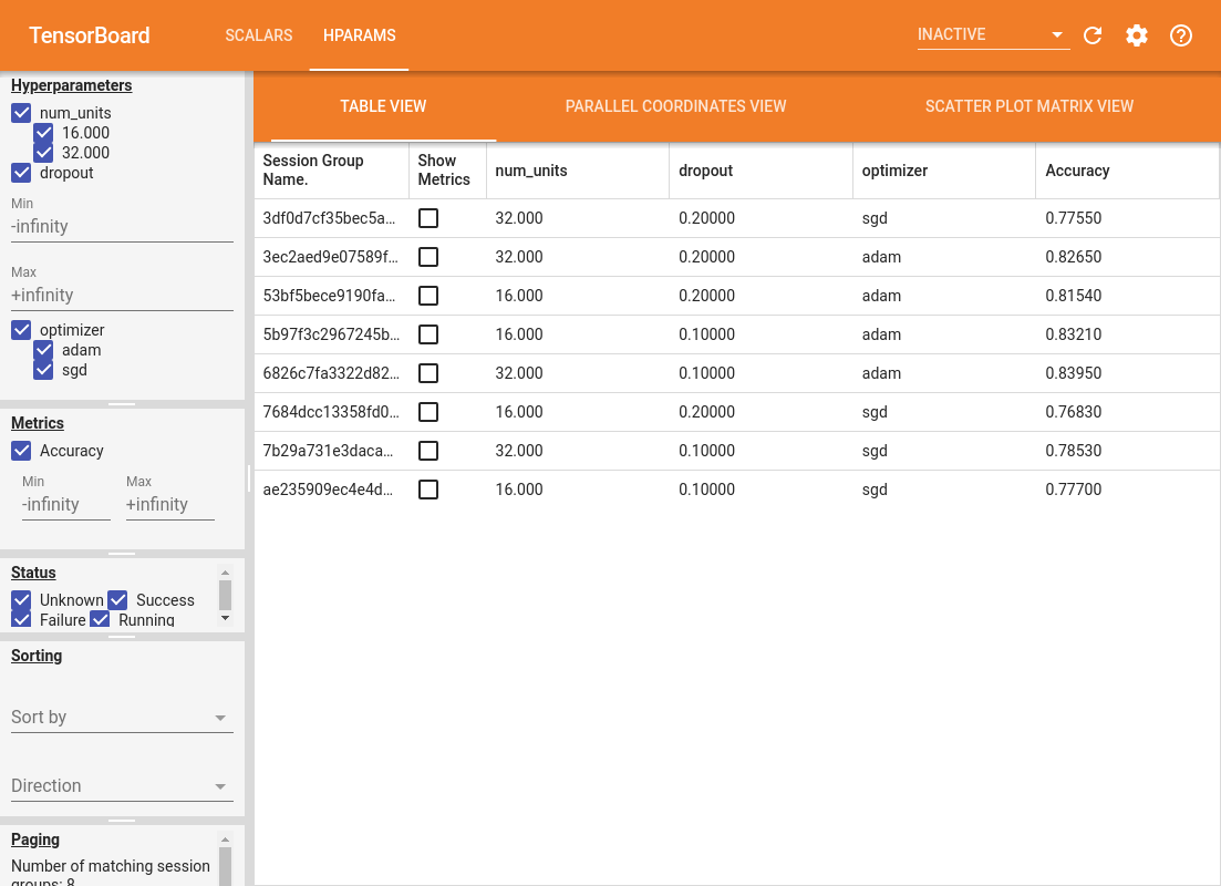
The left pane of the dashboard provides filtering capabilities that are active across all the views in the HParams dashboard:
- Filter which hyperparameters/metrics are shown in the dashboard
- Filter which hyperparameter/metrics values are shown in the dashboard
- Filter on run status (running, success, ...)
- Sort by hyperparameter/metric in the table view
- Number of session groups to show (useful for performance when there are many experiments)
The HParams dashboard has three different views, with various useful information:
- The Table View lists the runs, their hyperparameters, and their metrics.
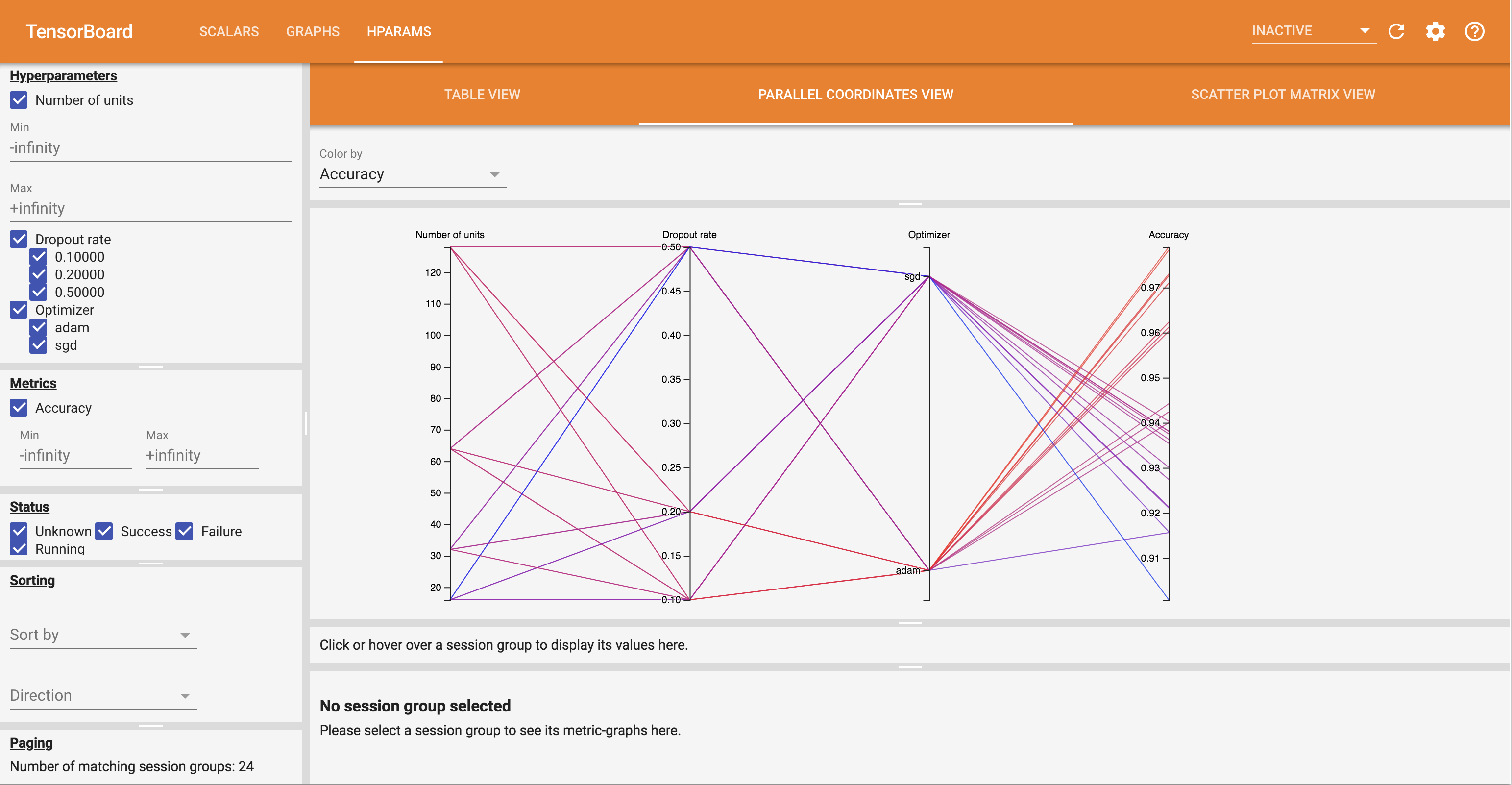
- The Parallel Coordinates View shows each run as a line going through an axis for each hyperparemeter and metric. Click and drag the mouse on any axis to mark a region which will highlight only the runs that pass through it. This can be useful for identifying which groups of hyperparameters are most important. The axes themselves can be re-ordered by dragging them.
- The Scatter Plot View shows plots comparing each hyperparameter/metric with each metric. This can help identify correlations. Click and drag to select a region in a specific plot and highlight those sessions across the other plots.
A table row, a parallel coordinates line, and a scatter plot market can be clicked to see a plot of the metrics as a function of training steps for that session (although in this tutorial only one step is used for each run).
To further explore the capabilities of the HParams dashboard, download a set of pregenerated logs with more experiments:
wget -q 'https://storage.googleapis.com/download.tensorflow.org/tensorboard/hparams_demo_logs.zip'unzip -q hparams_demo_logs.zip -d logs/hparam_demo
View these logs in TensorBoard:
%tensorboard --logdir logs/hparam_demo
You can try out the different views in the HParams dashboard.
For example, by going to the parallel coordinates view and clicking and dragging on the accuracy axis, you can select the runs with the highest accuracy. As these runs pass through 'adam' in the optimizer axis, you can conclude that 'adam' performed better than 'sgd' on these experiments.