
| | |  Voir la source sur GitHub Voir la source sur GitHub | |
Ce tutoriel de classification texte forme un réseau de neurones récurrent sur le IMDB grand ensemble de données critique de film pour l' analyse des sentiments.
Installer
import numpy as np

import tensorflow_datasets as tfds
import tensorflow as tf

tfds.disable_progress_bar()
Importation matplotlib et créer une fonction d'aide aux graphes de terrain:
import matplotlib.pyplot as plt


def plot_graphs(history, metric):
  plt.plot(history.history[metric])
  plt.plot(history.history['val_'+metric], '')
  plt.xlabel("Epochs")
  plt.ylabel(metric)
  plt.legend([metric, 'val_'+metric])
Configurer le pipeline d'entrée
Le IMDB grand ensemble de données critique de film est un ensemble de données tous les commentaires classification binaire ont soit positif ou sentiment négatif.
Télécharger le jeu de données à l' aide TFDS . Voir le tutoriel texte de chargement pour plus de détails sur la façon de charger ce type de données manuellement.
dataset, info = tfds.load('imdb_reviews', with_info=True,
                          as_supervised=True)
train_dataset, test_dataset = dataset['train'], dataset['test']

train_dataset.element_spec
(TensorSpec(shape=(), dtype=tf.string, name=None),
 TensorSpec(shape=(), dtype=tf.int64, name=None))
Initialement, cela renvoie un ensemble de données de (texte, paires d'étiquettes):
for example, label in train_dataset.take(1):
  print('text: ', example.numpy())
  print('label: ', label.numpy())
text:  b"This was an absolutely terrible movie. Don't be lured in by Christopher Walken or Michael Ironside. Both are great actors, but this must simply be their worst role in history. Even their great acting could not redeem this movie's ridiculous storyline. This movie is an early nineties US propaganda piece. The most pathetic scenes were those when the Columbian rebels were making their cases for revolutions. Maria Conchita Alonso appeared phony, and her pseudo-love affair with Walken was nothing but a pathetic emotional plug in a movie that was devoid of any real meaning. I am disappointed that there are movies like this, ruining actor's like Christopher Walken's good name. I could barely sit through it."
label:  0
Lecture aléatoire suivant les données de formation et de créer des lots de ces (text, label) paires:
BUFFER_SIZE = 10000
BATCH_SIZE = 64
train_dataset = train_dataset.shuffle(BUFFER_SIZE).batch(BATCH_SIZE).prefetch(tf.data.AUTOTUNE)
test_dataset = test_dataset.batch(BATCH_SIZE).prefetch(tf.data.AUTOTUNE)
for example, label in train_dataset.take(1):
  print('texts: ', example.numpy()[:3])
  print()
  print('labels: ', label.numpy()[:3])
texts:  [b'This is arguably the worst film I have ever seen, and I have quite an appetite for awful (and good) movies. It could (just) have managed a kind of adolescent humour if it had been consistently tongue-in-cheek --\xc3\xa0 la ROCKY HORROR PICTURE SHOW, which was really very funny. Other movies, like PLAN NINE FROM OUTER SPACE, manage to be funny while (apparently) trying to be serious. As to the acting, it looks like they rounded up brain-dead teenagers and asked them to ad-lib the whole production. Compared to them, Tom Cruise looks like Alec Guinness. There was one decent interpretation -- that of the older ghoul-busting broad on the motorcycle.'
 b"I saw this film in the worst possible circumstance. I'd already missed 15 minutes when I woke up to it on an international flight between Sydney and Seoul. I didn't know what I was watching, I thought maybe it was a movie of the week, but quickly became riveted by the performance of the lead actress playing a young woman who's child had been kidnapped. The premise started taking twist and turns I didn't see coming and by the end credits I was scrambling through the the in-flight guide to figure out what I had just watched. Turns out I was belatedly discovering Do-yeon Jeon who'd won Best Actress at Cannes for the role. I don't know if Secret Sunshine is typical of Korean cinema but I'm off to the DVD store to discover more."
 b"Hello. I am Paul Raddick, a.k.a. Panic Attack of WTAF, Channel 29 in Philadelphia. Let me tell you about this god awful movie that powered on Adam Sandler's film career but was digitized after a short time.<br /><br />Going Overboard is about an aspiring comedian played by Sandler who gets a job on a cruise ship and fails...or so I thought. Sandler encounters babes that like History of the World Part 1 and Rebound. The babes were supposed to be engaged, but, actually, they get executed by Sawtooth, the meanest cannibal the world has ever known. Adam Sandler fared bad in Going Overboard, but fared better in Big Daddy, Billy Madison, and Jen Leone's favorite, 50 First Dates. Man, Drew Barrymore was one hot chick. Spanglish is red hot, Going Overboard ain't Dooley squat! End of file."]

labels:  [0 1 0]
Créer l'encodeur de texte
Le texte brut chargé par tfds doit être traitée avant de pouvoir être utilisé dans un modèle. La façon la plus simple au texte de processus de formation utilise la TextVectorization couche. Cette couche a de nombreuses fonctionnalités, mais ce didacticiel s'en tient au comportement par défaut.
Créer la couche, et de transmettre le texte de l'ensemble de données de la couche .adapt méthode:
VOCAB_SIZE = 1000
encoder = tf.keras.layers.TextVectorization(
    max_tokens=VOCAB_SIZE)
encoder.adapt(train_dataset.map(lambda text, label: text))
La .adapt méthode définit le vocabulaire de la couche. Voici les 20 premiers jetons. Après le remplissage et les jetons inconnus, ils sont triés par fréquence :
vocab = np.array(encoder.get_vocabulary())
vocab[:20]
array(['', '[UNK]', 'the', 'and', 'a', 'of', 'to', 'is', 'in', 'it', 'i',
       'this', 'that', 'br', 'was', 'as', 'for', 'with', 'movie', 'but'],
      dtype='<U14')
Une fois le vocabulaire défini, la couche peut encoder le texte en index. Les tenseurs des indices 0 rembourrées à la plus longue séquence dans le lot (sauf si vous définissez un fixe output_sequence_length ):
encoded_example = encoder(example)[:3].numpy()
encoded_example
array([[ 11,   7,   1, ...,   0,   0,   0],
       [ 10, 208,  11, ...,   0,   0,   0],
       [  1,  10, 237, ...,   0,   0,   0]])
Avec les paramètres par défaut, le processus n'est pas complètement réversible. Il y a trois raisons principales à cela :
- La valeur par défaut pour
preprocessing.TextVectorizationl »standardizeargument est"lower_and_strip_punctuation". - La taille limitée du vocabulaire et l'absence de solution de secours basée sur les caractères donnent lieu à des jetons inconnus.
for n in range(3):
  print("Original: ", example[n].numpy())
  print("Round-trip: ", " ".join(vocab[encoded_example[n]]))
  print()
Original:  b'This is arguably the worst film I have ever seen, and I have quite an appetite for awful (and good) movies. It could (just) have managed a kind of adolescent humour if it had been consistently tongue-in-cheek --\xc3\xa0 la ROCKY HORROR PICTURE SHOW, which was really very funny. Other movies, like PLAN NINE FROM OUTER SPACE, manage to be funny while (apparently) trying to be serious. As to the acting, it looks like they rounded up brain-dead teenagers and asked them to ad-lib the whole production. Compared to them, Tom Cruise looks like Alec Guinness. There was one decent interpretation -- that of the older ghoul-busting broad on the motorcycle.'
Round-trip:  this is [UNK] the worst film i have ever seen and i have quite an [UNK] for awful and good movies it could just have [UNK] a kind of [UNK] [UNK] if it had been [UNK] [UNK] [UNK] la [UNK] horror picture show which was really very funny other movies like [UNK] [UNK] from [UNK] space [UNK] to be funny while apparently trying to be serious as to the acting it looks like they [UNK] up [UNK] [UNK] and [UNK] them to [UNK] the whole production [UNK] to them tom [UNK] looks like [UNK] [UNK] there was one decent [UNK] that of the older [UNK] [UNK] on the [UNK]

Original:  b"I saw this film in the worst possible circumstance. I'd already missed 15 minutes when I woke up to it on an international flight between Sydney and Seoul. I didn't know what I was watching, I thought maybe it was a movie of the week, but quickly became riveted by the performance of the lead actress playing a young woman who's child had been kidnapped. The premise started taking twist and turns I didn't see coming and by the end credits I was scrambling through the the in-flight guide to figure out what I had just watched. Turns out I was belatedly discovering Do-yeon Jeon who'd won Best Actress at Cannes for the role. I don't know if Secret Sunshine is typical of Korean cinema but I'm off to the DVD store to discover more."
Round-trip:  i saw this film in the worst possible [UNK] id already [UNK] [UNK] minutes when i [UNK] up to it on an [UNK] [UNK] between [UNK] and [UNK] i didnt know what i was watching i thought maybe it was a movie of the [UNK] but quickly became [UNK] by the performance of the lead actress playing a young woman whos child had been [UNK] the premise started taking twist and turns i didnt see coming and by the end credits i was [UNK] through the the [UNK] [UNK] to figure out what i had just watched turns out i was [UNK] [UNK] [UNK] [UNK] [UNK] [UNK] best actress at [UNK] for the role i dont know if secret [UNK] is typical of [UNK] cinema but im off to the dvd [UNK] to [UNK] more

Original:  b"Hello. I am Paul Raddick, a.k.a. Panic Attack of WTAF, Channel 29 in Philadelphia. Let me tell you about this god awful movie that powered on Adam Sandler's film career but was digitized after a short time.<br /><br />Going Overboard is about an aspiring comedian played by Sandler who gets a job on a cruise ship and fails...or so I thought. Sandler encounters babes that like History of the World Part 1 and Rebound. The babes were supposed to be engaged, but, actually, they get executed by Sawtooth, the meanest cannibal the world has ever known. Adam Sandler fared bad in Going Overboard, but fared better in Big Daddy, Billy Madison, and Jen Leone's favorite, 50 First Dates. Man, Drew Barrymore was one hot chick. Spanglish is red hot, Going Overboard ain't Dooley squat! End of file."
Round-trip:  [UNK] i am paul [UNK] [UNK] [UNK] [UNK] of [UNK] [UNK] [UNK] in [UNK] let me tell you about this god awful movie that [UNK] on [UNK] [UNK] film career but was [UNK] after a short [UNK] br going [UNK] is about an [UNK] [UNK] played by [UNK] who gets a job on a [UNK] [UNK] and [UNK] so i thought [UNK] [UNK] [UNK] that like history of the world part 1 and [UNK] the [UNK] were supposed to be [UNK] but actually they get [UNK] by [UNK] the [UNK] [UNK] the world has ever known [UNK] [UNK] [UNK] bad in going [UNK] but [UNK] better in big [UNK] [UNK] [UNK] and [UNK] [UNK] favorite [UNK] first [UNK] man [UNK] [UNK] was one hot [UNK] [UNK] is red hot going [UNK] [UNK] [UNK] [UNK] end of [UNK]
Créer le modèle
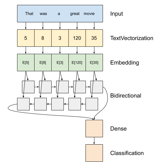
Ci-dessus, un schéma du modèle.
Ce modèle peut être construit comme
tf.keras.Sequential.La première couche est le
encoder, qui convertit le texte en une séquence d'indices de jeton.Après l'encodeur se trouve une couche d'intégration. Une couche d'incorporation stocke un vecteur par mot. Lorsqu'il est appelé, il convertit les séquences d'indices de mots en séquences de vecteurs. Ces vecteurs sont entraînables. Après apprentissage (sur suffisamment de données), les mots ayant des significations similaires ont souvent des vecteurs similaires.
Cet indice-recherche est beaucoup plus efficace que l'opération consistant à faire passer l' équivalent d' un vecteur codé d' un chaud à travers un
tf.keras.layers.Densecouche.Un réseau de neurones récurrents (RNN) traite l'entrée de séquence en itérant à travers les éléments. Les RNN transmettent les sorties d'un pas de temps à leur entrée au pas de temps suivant.
Le
tf.keras.layers.Bidirectionalemballage peut également être utilisé avec une couche RNN. Cela propage l'entrée vers l'avant et vers l'arrière à travers la couche RNN, puis concatène la sortie finale.Le principal avantage d'un RNN bidirectionnel est que le signal du début de l'entrée n'a pas besoin d'être traité tout au long de chaque pas de temps pour affecter la sortie.
Le principal inconvénient d'un RNN bidirectionnel est que vous ne pouvez pas diffuser efficacement les prédictions car des mots sont ajoutés à la fin.
Après la RNN a converti la séquence à un seul vecteur les deux
layers.Densefaire un peu de traitement final, et convertir de cette représentation vectorielle à un seul logit comme la sortie de classification.
Le code pour implémenter ceci est ci-dessous:
model = tf.keras.Sequential([
    encoder,
    tf.keras.layers.Embedding(
        input_dim=len(encoder.get_vocabulary()),
        output_dim=64,
        # Use masking to handle the variable sequence lengths
        mask_zero=True),
    tf.keras.layers.Bidirectional(tf.keras.layers.LSTM(64)),
    tf.keras.layers.Dense(64, activation='relu'),
    tf.keras.layers.Dense(1)
])
Veuillez noter que le modèle séquentiel Keras est utilisé ici car toutes les couches du modèle n'ont qu'une seule entrée et produisent une seule sortie. Si vous souhaitez utiliser une couche RNN avec état, vous pouvez créer votre modèle avec l'API fonctionnelle Keras ou un sous-classement de modèle afin de pouvoir récupérer et réutiliser les états de la couche RNN. S'il vous plaît vérifier Guide Keras RNN pour plus de détails.
La couche d' enrobage utilisations de masquage pour gérer les différentes longueurs de séquence. Toutes les couches après le Embedding masquage de support:
print([layer.supports_masking for layer in model.layers])
[False, True, True, True, True]
Pour confirmer que cela fonctionne comme prévu, évaluez une phrase deux fois. Tout d'abord, seul donc il n'y a pas de rembourrage à masquer :
# predict on a sample text without padding.

sample_text = ('The movie was cool. The animation and the graphics '
               'were out of this world. I would recommend this movie.')
predictions = model.predict(np.array([sample_text]))
print(predictions[0])
[-0.00012211]
Maintenant, évaluez-le à nouveau dans un lot avec une phrase plus longue. Le résultat doit être identique :
# predict on a sample text with padding

padding = "the " * 2000
predictions = model.predict(np.array([sample_text, padding]))
print(predictions[0])
[-0.00012211]
Compilez le modèle Keras pour configurer le processus de formation :
model.compile(loss=tf.keras.losses.BinaryCrossentropy(from_logits=True),
              optimizer=tf.keras.optimizers.Adam(1e-4),
              metrics=['accuracy'])
Former le modèle
history = model.fit(train_dataset, epochs=10,
                    validation_data=test_dataset,
                    validation_steps=30)
Epoch 1/10
391/391 [==============================] - 39s 84ms/step - loss: 0.6454 - accuracy: 0.5630 - val_loss: 0.4888 - val_accuracy: 0.7568
Epoch 2/10
391/391 [==============================] - 30s 75ms/step - loss: 0.3925 - accuracy: 0.8200 - val_loss: 0.3663 - val_accuracy: 0.8464
Epoch 3/10
391/391 [==============================] - 30s 75ms/step - loss: 0.3319 - accuracy: 0.8525 - val_loss: 0.3402 - val_accuracy: 0.8385
Epoch 4/10
391/391 [==============================] - 30s 75ms/step - loss: 0.3183 - accuracy: 0.8616 - val_loss: 0.3289 - val_accuracy: 0.8438
Epoch 5/10
391/391 [==============================] - 30s 75ms/step - loss: 0.3088 - accuracy: 0.8656 - val_loss: 0.3254 - val_accuracy: 0.8646
Epoch 6/10
391/391 [==============================] - 32s 81ms/step - loss: 0.3043 - accuracy: 0.8686 - val_loss: 0.3242 - val_accuracy: 0.8521
Epoch 7/10
391/391 [==============================] - 30s 76ms/step - loss: 0.3019 - accuracy: 0.8696 - val_loss: 0.3315 - val_accuracy: 0.8609
Epoch 8/10
391/391 [==============================] - 32s 76ms/step - loss: 0.3007 - accuracy: 0.8688 - val_loss: 0.3245 - val_accuracy: 0.8609
Epoch 9/10
391/391 [==============================] - 31s 77ms/step - loss: 0.2981 - accuracy: 0.8707 - val_loss: 0.3294 - val_accuracy: 0.8599
Epoch 10/10
391/391 [==============================] - 31s 78ms/step - loss: 0.2969 - accuracy: 0.8742 - val_loss: 0.3218 - val_accuracy: 0.8547
test_loss, test_acc = model.evaluate(test_dataset)

print('Test Loss:', test_loss)
print('Test Accuracy:', test_acc)
391/391 [==============================] - 15s 38ms/step - loss: 0.3185 - accuracy: 0.8582
Test Loss: 0.3184521794319153
Test Accuracy: 0.8581600189208984
plt.figure(figsize=(16, 8))
plt.subplot(1, 2, 1)
plot_graphs(history, 'accuracy')
plt.ylim(None, 1)
plt.subplot(1, 2, 2)
plot_graphs(history, 'loss')
plt.ylim(0, None)
(0.0, 0.6627909764647484)

Exécutez une prédiction sur une nouvelle phrase :
Si la prédiction est >= 0.0, elle est positive sinon elle est négative.
sample_text = ('The movie was cool. The animation and the graphics '
               'were out of this world. I would recommend this movie.')
predictions = model.predict(np.array([sample_text]))
Empilez deux ou plusieurs couches LSTM
KERAS couches récurrentes ont deux modes disponibles qui sont contrôlés par le return_sequences argument du constructeur:
Si
Falsequ'il ne renvoie que la dernière sortie pour chaque séquence d'entrée (un tenseur 2D de forme (batch_size, output_features)). Il s'agit de la valeur par défaut, utilisée dans le modèle précédent.Si
Trueles séquences complètes de sorties successives pour chaque timestep est retourné (un tenseur 3D de forme(batch_size, timesteps, output_features)pas de(batch_size, timesteps, output_features)).
Voici ce que le flux de regards d'information comme avec return_sequences=True :
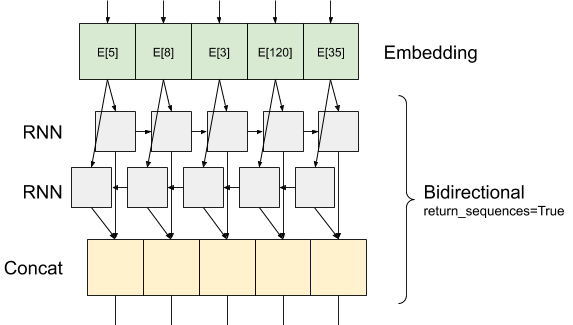
La chose intéressante à propos de l' utilisation d' un RNN avec return_sequences=True est que la sortie a encore 3 axes, comme l'entrée, donc il peut être transmis à une autre couche RNN, comme ceci:
model = tf.keras.Sequential([
    encoder,
    tf.keras.layers.Embedding(len(encoder.get_vocabulary()), 64, mask_zero=True),
    tf.keras.layers.Bidirectional(tf.keras.layers.LSTM(64,  return_sequences=True)),
    tf.keras.layers.Bidirectional(tf.keras.layers.LSTM(32)),
    tf.keras.layers.Dense(64, activation='relu'),
    tf.keras.layers.Dropout(0.5),
    tf.keras.layers.Dense(1)
])
model.compile(loss=tf.keras.losses.BinaryCrossentropy(from_logits=True),
              optimizer=tf.keras.optimizers.Adam(1e-4),
              metrics=['accuracy'])
history = model.fit(train_dataset, epochs=10,
                    validation_data=test_dataset,
                    validation_steps=30)
Epoch 1/10
391/391 [==============================] - 71s 149ms/step - loss: 0.6502 - accuracy: 0.5625 - val_loss: 0.4923 - val_accuracy: 0.7573
Epoch 2/10
391/391 [==============================] - 55s 138ms/step - loss: 0.4067 - accuracy: 0.8198 - val_loss: 0.3727 - val_accuracy: 0.8271
Epoch 3/10
391/391 [==============================] - 54s 136ms/step - loss: 0.3417 - accuracy: 0.8543 - val_loss: 0.3343 - val_accuracy: 0.8510
Epoch 4/10
391/391 [==============================] - 53s 134ms/step - loss: 0.3242 - accuracy: 0.8607 - val_loss: 0.3268 - val_accuracy: 0.8568
Epoch 5/10
391/391 [==============================] - 53s 135ms/step - loss: 0.3174 - accuracy: 0.8652 - val_loss: 0.3213 - val_accuracy: 0.8516
Epoch 6/10
391/391 [==============================] - 52s 132ms/step - loss: 0.3098 - accuracy: 0.8671 - val_loss: 0.3294 - val_accuracy: 0.8547
Epoch 7/10
391/391 [==============================] - 53s 134ms/step - loss: 0.3063 - accuracy: 0.8697 - val_loss: 0.3158 - val_accuracy: 0.8594
Epoch 8/10
391/391 [==============================] - 52s 132ms/step - loss: 0.3043 - accuracy: 0.8692 - val_loss: 0.3184 - val_accuracy: 0.8521
Epoch 9/10
391/391 [==============================] - 53s 133ms/step - loss: 0.3016 - accuracy: 0.8704 - val_loss: 0.3208 - val_accuracy: 0.8609
Epoch 10/10
391/391 [==============================] - 54s 136ms/step - loss: 0.2975 - accuracy: 0.8740 - val_loss: 0.3301 - val_accuracy: 0.8651
test_loss, test_acc = model.evaluate(test_dataset)

print('Test Loss:', test_loss)
print('Test Accuracy:', test_acc)
391/391 [==============================] - 26s 65ms/step - loss: 0.3293 - accuracy: 0.8646
Test Loss: 0.329334557056427
Test Accuracy: 0.8646399974822998
# predict on a sample text without padding.

sample_text = ('The movie was not good. The animation and the graphics '
               'were terrible. I would not recommend this movie.')
predictions = model.predict(np.array([sample_text]))
print(predictions)
[[-1.6796288]]
plt.figure(figsize=(16, 6))
plt.subplot(1, 2, 1)
plot_graphs(history, 'accuracy')
plt.subplot(1, 2, 2)
plot_graphs(history, 'loss')

Découvrez les autres couches récurrentes existantes telles que les couches GRU .
Si vous interestied dans la construction RNNs personnalisés, consultez le Guide Keras RNN .