
Copyright 2023 The TF-Agents Authors.
|
|
|
 View source on GitHub
|
|
Introduction
This example shows how to train a DQN (Deep Q Networks) agent on the Cartpole environment using the TF-Agents library.
It will walk you through all the components in a Reinforcement Learning (RL) pipeline for training, evaluation and data collection.
To run this code live, click the 'Run in Google Colab' link above.
Setup
If you haven't installed the following dependencies, run:
sudo apt-get updatesudo apt-get install -y xvfb ffmpeg freeglut3-devpip install 'imageio==2.4.0'pip install pyvirtualdisplaypip install tf-agents[reverb]pip install pygletpip install tf-keras
import os
# Keep using keras-2 (tf-keras) rather than keras-3 (keras).
os.environ['TF_USE_LEGACY_KERAS'] = '1'
from __future__ import absolute_import, division, print_function

import base64
import imageio
import IPython
import matplotlib
import matplotlib.pyplot as plt
import numpy as np
import PIL.Image
import pyvirtualdisplay
import reverb

import tensorflow as tf

from tf_agents.agents.dqn import dqn_agent
from tf_agents.drivers import py_driver
from tf_agents.environments import suite_gym
from tf_agents.environments import tf_py_environment
from tf_agents.eval import metric_utils
from tf_agents.metrics import tf_metrics
from tf_agents.networks import sequential
from tf_agents.policies import py_tf_eager_policy
from tf_agents.policies import random_tf_policy
from tf_agents.replay_buffers import reverb_replay_buffer
from tf_agents.replay_buffers import reverb_utils
from tf_agents.trajectories import trajectory
from tf_agents.specs import tensor_spec
from tf_agents.utils import common
2023-12-22 13:55:18.305379: E external/local_xla/xla/stream_executor/cuda/cuda_dnn.cc:9261] Unable to register cuDNN factory: Attempting to register factory for plugin cuDNN when one has already been registered
2023-12-22 13:55:18.305427: E external/local_xla/xla/stream_executor/cuda/cuda_fft.cc:607] Unable to register cuFFT factory: Attempting to register factory for plugin cuFFT when one has already been registered
2023-12-22 13:55:18.307063: E external/local_xla/xla/stream_executor/cuda/cuda_blas.cc:1515] Unable to register cuBLAS factory: Attempting to register factory for plugin cuBLAS when one has already been registered
# Set up a virtual display for rendering OpenAI gym environments.
display = pyvirtualdisplay.Display(visible=0, size=(1400, 900)).start()
tf.version.VERSION
'2.15.0'
Hyperparameters
num_iterations = 20000 # @param {type:"integer"}

initial_collect_steps = 100  # @param {type:"integer"}
collect_steps_per_iteration =   1# @param {type:"integer"}
replay_buffer_max_length = 100000  # @param {type:"integer"}

batch_size = 64  # @param {type:"integer"}
learning_rate = 1e-3  # @param {type:"number"}
log_interval = 200  # @param {type:"integer"}

num_eval_episodes = 10  # @param {type:"integer"}
eval_interval = 1000  # @param {type:"integer"}
Environment
In Reinforcement Learning (RL), an environment represents the task or problem to be solved. Standard environments can be created in TF-Agents using tf_agents.environments suites. TF-Agents has suites for loading environments from sources such as the OpenAI Gym, Atari, and DM Control.
Load the CartPole environment from the OpenAI Gym suite.
env_name = 'CartPole-v0'
env = suite_gym.load(env_name)
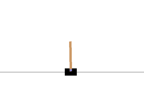
You can render this environment to see how it looks. A free-swinging pole is attached to a cart. The goal is to move the cart right or left in order to keep the pole pointing up.
env.reset()
PIL.Image.fromarray(env.render())

The environment.step method takes an action in the environment and returns a TimeStep tuple containing the next observation of the environment and the reward for the action.
The time_step_spec() method returns the specification for the TimeStep tuple. Its observation attribute shows the shape of observations, the data types, and the ranges of allowed values. The reward attribute shows the same details for the reward.
print('Observation Spec:')
print(env.time_step_spec().observation)
Observation Spec:
BoundedArraySpec(shape=(4,), dtype=dtype('float32'), name='observation', minimum=[-4.8000002e+00 -3.4028235e+38 -4.1887903e-01 -3.4028235e+38], maximum=[4.8000002e+00 3.4028235e+38 4.1887903e-01 3.4028235e+38])
print('Reward Spec:')
print(env.time_step_spec().reward)
Reward Spec:
ArraySpec(shape=(), dtype=dtype('float32'), name='reward')
The action_spec() method returns the shape, data types, and allowed values of valid actions.
print('Action Spec:')
print(env.action_spec())
Action Spec:
BoundedArraySpec(shape=(), dtype=dtype('int64'), name='action', minimum=0, maximum=1)
In the Cartpole environment:
observationis an array of 4 floats:- the position and velocity of the cart
- the angular position and velocity of the pole
rewardis a scalar float valueactionis a scalar integer with only two possible values:0— "move left"1— "move right"
time_step = env.reset()
print('Time step:')
print(time_step)

action = np.array(1, dtype=np.int32)

next_time_step = env.step(action)
print('Next time step:')
print(next_time_step)
Time step:
TimeStep(
{'step_type': array(0, dtype=int32),
 'reward': array(0., dtype=float32),
 'discount': array(1., dtype=float32),
 'observation': array([ 0.0365577 , -0.00826731, -0.02852953, -0.02371309], dtype=float32)})
Next time step:
TimeStep(
{'step_type': array(1, dtype=int32),
 'reward': array(1., dtype=float32),
 'discount': array(1., dtype=float32),
 'observation': array([ 0.03639235,  0.18725191, -0.02900379, -0.32525912], dtype=float32)})
Usually two environments are instantiated: one for training and one for evaluation.
train_py_env = suite_gym.load(env_name)
eval_py_env = suite_gym.load(env_name)
The Cartpole environment, like most environments, is written in pure Python. This is converted to TensorFlow using the TFPyEnvironment wrapper.
The original environment's API uses Numpy arrays. The TFPyEnvironment converts these to Tensors to make it compatible with Tensorflow agents and policies.
train_env = tf_py_environment.TFPyEnvironment(train_py_env)
eval_env = tf_py_environment.TFPyEnvironment(eval_py_env)
Agent
The algorithm used to solve an RL problem is represented by an Agent. TF-Agents provides standard implementations of a variety of Agents, including:
The DQN agent can be used in any environment which has a discrete action space.
At the heart of a DQN Agent is a QNetwork, a neural network model that can learn to predict QValues (expected returns) for all actions, given an observation from the environment.
We will use tf_agents.networks. to create a QNetwork. The network will consist of a sequence of tf.keras.layers.Dense layers, where the final layer will have 1 output for each possible action.
fc_layer_params = (100, 50)
action_tensor_spec = tensor_spec.from_spec(env.action_spec())
num_actions = action_tensor_spec.maximum - action_tensor_spec.minimum + 1

# Define a helper function to create Dense layers configured with the right
# activation and kernel initializer.
def dense_layer(num_units):
  return tf.keras.layers.Dense(
      num_units,
      activation=tf.keras.activations.relu,
      kernel_initializer=tf.keras.initializers.VarianceScaling(
          scale=2.0, mode='fan_in', distribution='truncated_normal'))

# QNetwork consists of a sequence of Dense layers followed by a dense layer
# with `num_actions` units to generate one q_value per available action as
# its output.
dense_layers = [dense_layer(num_units) for num_units in fc_layer_params]
q_values_layer = tf.keras.layers.Dense(
    num_actions,
    activation=None,
    kernel_initializer=tf.keras.initializers.RandomUniform(
        minval=-0.03, maxval=0.03),
    bias_initializer=tf.keras.initializers.Constant(-0.2))
q_net = sequential.Sequential(dense_layers + [q_values_layer])
Now use tf_agents.agents.dqn.dqn_agent to instantiate a DqnAgent. In addition to the time_step_spec, action_spec and the QNetwork, the agent constructor also requires an optimizer (in this case, AdamOptimizer), a loss function, and an integer step counter.
optimizer = tf.keras.optimizers.Adam(learning_rate=learning_rate)

train_step_counter = tf.Variable(0)

agent = dqn_agent.DqnAgent(
    train_env.time_step_spec(),
    train_env.action_spec(),
    q_network=q_net,
    optimizer=optimizer,
    td_errors_loss_fn=common.element_wise_squared_loss,
    train_step_counter=train_step_counter)

agent.initialize()
Policies
A policy defines the way an agent acts in an environment. Typically, the goal of reinforcement learning is to train the underlying model until the policy produces the desired outcome.
In this tutorial:
- The desired outcome is keeping the pole balanced upright over the cart.
- The policy returns an action (left or right) for each
time_stepobservation.
Agents contain two policies:
agent.policy— The main policy that is used for evaluation and deployment.agent.collect_policy— A second policy that is used for data collection.
eval_policy = agent.policy
collect_policy = agent.collect_policy
Policies can be created independently of agents. For example, use tf_agents.policies.random_tf_policy to create a policy which will randomly select an action for each time_step.
random_policy = random_tf_policy.RandomTFPolicy(train_env.time_step_spec(),
                                                train_env.action_spec())
To get an action from a policy, call the policy.action(time_step) method. The time_step contains the observation from the environment. This method returns a PolicyStep, which is a named tuple with three components:
action— the action to be taken (in this case,0or1)state— used for stateful (that is, RNN-based) policiesinfo— auxiliary data, such as log probabilities of actions
example_environment = tf_py_environment.TFPyEnvironment(
    suite_gym.load('CartPole-v0'))
time_step = example_environment.reset()
random_policy.action(time_step)
PolicyStep(action=<tf.Tensor: shape=(1,), dtype=int64, numpy=array([1])>, state=(), info=())
Metrics and Evaluation
The most common metric used to evaluate a policy is the average return. The return is the sum of rewards obtained while running a policy in an environment for an episode. Several episodes are run, creating an average return.
The following function computes the average return of a policy, given the policy, environment, and a number of episodes.
def compute_avg_return(environment, policy, num_episodes=10):

  total_return = 0.0
  for _ in range(num_episodes):

    time_step = environment.reset()
    episode_return = 0.0

    while not time_step.is_last():
      action_step = policy.action(time_step)
      time_step = environment.step(action_step.action)
      episode_return += time_step.reward
    total_return += episode_return

  avg_return = total_return / num_episodes
  return avg_return.numpy()[0]


# See also the metrics module for standard implementations of different metrics.
# https://github.com/tensorflow/agents/tree/master/tf_agents/metrics
Running this computation on the random_policy shows a baseline performance in the environment.
compute_avg_return(eval_env, random_policy, num_eval_episodes)
23.5
Replay Buffer
In order to keep track of the data collected from the environment, we will use Reverb, an efficient, extensible, and easy-to-use replay system by Deepmind. It stores experience data when we collect trajectories and is consumed during training.
This replay buffer is constructed using specs describing the tensors that are to be stored, which can be obtained from the agent using agent.collect_data_spec.
table_name = 'uniform_table'
replay_buffer_signature = tensor_spec.from_spec(
      agent.collect_data_spec)
replay_buffer_signature = tensor_spec.add_outer_dim(
    replay_buffer_signature)

table = reverb.Table(
    table_name,
    max_size=replay_buffer_max_length,
    sampler=reverb.selectors.Uniform(),
    remover=reverb.selectors.Fifo(),
    rate_limiter=reverb.rate_limiters.MinSize(1),
    signature=replay_buffer_signature)

reverb_server = reverb.Server([table])

replay_buffer = reverb_replay_buffer.ReverbReplayBuffer(
    agent.collect_data_spec,
    table_name=table_name,
    sequence_length=2,
    local_server=reverb_server)

rb_observer = reverb_utils.ReverbAddTrajectoryObserver(
  replay_buffer.py_client,
  table_name,
  sequence_length=2)
[reverb/cc/platform/tfrecord_checkpointer.cc:162]  Initializing TFRecordCheckpointer in /tmpfs/tmp/tmpcvnrrkpg.
[reverb/cc/platform/tfrecord_checkpointer.cc:565] Loading latest checkpoint from /tmpfs/tmp/tmpcvnrrkpg
[reverb/cc/platform/default/server.cc:71] Started replay server on port 46351
For most agents, collect_data_spec is a named tuple called Trajectory, containing the specs for observations, actions, rewards, and other items.
agent.collect_data_spec
Trajectory(
{'step_type': TensorSpec(shape=(), dtype=tf.int32, name='step_type'),
 'observation': BoundedTensorSpec(shape=(4,), dtype=tf.float32, name='observation', minimum=array([-4.8000002e+00, -3.4028235e+38, -4.1887903e-01, -3.4028235e+38],
      dtype=float32), maximum=array([4.8000002e+00, 3.4028235e+38, 4.1887903e-01, 3.4028235e+38],
      dtype=float32)),
 'action': BoundedTensorSpec(shape=(), dtype=tf.int64, name='action', minimum=array(0), maximum=array(1)),
 'policy_info': (),
 'next_step_type': TensorSpec(shape=(), dtype=tf.int32, name='step_type'),
 'reward': TensorSpec(shape=(), dtype=tf.float32, name='reward'),
 'discount': BoundedTensorSpec(shape=(), dtype=tf.float32, name='discount', minimum=array(0., dtype=float32), maximum=array(1., dtype=float32))})
agent.collect_data_spec._fields
('step_type',
 'observation',
 'action',
 'policy_info',
 'next_step_type',
 'reward',
 'discount')
Data Collection
Now execute the random policy in the environment for a few steps, recording the data in the replay buffer.
Here we are using 'PyDriver' to run the experience collecting loop. You can learn more about TF Agents driver in our drivers tutorial.
py_driver.PyDriver(
    env,
    py_tf_eager_policy.PyTFEagerPolicy(
      random_policy, use_tf_function=True),
    [rb_observer],
    max_steps=initial_collect_steps).run(train_py_env.reset())
(TimeStep(
 {'step_type': array(1, dtype=int32),
  'reward': array(1., dtype=float32),
  'discount': array(1., dtype=float32),
  'observation': array([-0.03368392,  0.18694404, -0.00172193, -0.24534112], dtype=float32)}),
 ())
The replay buffer is now a collection of Trajectories.
# For the curious:
# Uncomment to peel one of these off and inspect it.
# iter(replay_buffer.as_dataset()).next()
The agent needs access to the replay buffer. This is provided by creating an iterable tf.data.Dataset pipeline which will feed data to the agent.
Each row of the replay buffer only stores a single observation step. But since the DQN Agent needs both the current and next observation to compute the loss, the dataset pipeline will sample two adjacent rows for each item in the batch (num_steps=2).
This dataset is also optimized by running parallel calls and prefetching data.
# Dataset generates trajectories with shape [Bx2x...]
dataset = replay_buffer.as_dataset(
    num_parallel_calls=3,
    sample_batch_size=batch_size,
    num_steps=2).prefetch(3)

dataset
<_PrefetchDataset element_spec=(Trajectory(
{'step_type': TensorSpec(shape=(64, 2), dtype=tf.int32, name=None),
 'observation': TensorSpec(shape=(64, 2, 4), dtype=tf.float32, name=None),
 'action': TensorSpec(shape=(64, 2), dtype=tf.int64, name=None),
 'policy_info': (),
 'next_step_type': TensorSpec(shape=(64, 2), dtype=tf.int32, name=None),
 'reward': TensorSpec(shape=(64, 2), dtype=tf.float32, name=None),
 'discount': TensorSpec(shape=(64, 2), dtype=tf.float32, name=None)}), SampleInfo(key=TensorSpec(shape=(64, 2), dtype=tf.uint64, name=None), probability=TensorSpec(shape=(64, 2), dtype=tf.float64, name=None), table_size=TensorSpec(shape=(64, 2), dtype=tf.int64, name=None), priority=TensorSpec(shape=(64, 2), dtype=tf.float64, name=None), times_sampled=TensorSpec(shape=(64, 2), dtype=tf.int32, name=None)))>
iterator = iter(dataset)
print(iterator)
<tensorflow.python.data.ops.iterator_ops.OwnedIterator object at 0x7f048a8c8dc0>
# For the curious:
# Uncomment to see what the dataset iterator is feeding to the agent.
# Compare this representation of replay data
# to the collection of individual trajectories shown earlier.

# iterator.next()
Training the agent
Two things must happen during the training loop:
- collect data from the environment
- use that data to train the agent's neural network(s)
This example also periodicially evaluates the policy and prints the current score.
The following will take ~5 minutes to run.
try:
  %%time
except:
  pass

# (Optional) Optimize by wrapping some of the code in a graph using TF function.
agent.train = common.function(agent.train)

# Reset the train step.
agent.train_step_counter.assign(0)

# Evaluate the agent's policy once before training.
avg_return = compute_avg_return(eval_env, agent.policy, num_eval_episodes)
returns = [avg_return]

# Reset the environment.
time_step = train_py_env.reset()

# Create a driver to collect experience.
collect_driver = py_driver.PyDriver(
    env,
    py_tf_eager_policy.PyTFEagerPolicy(
      agent.collect_policy, use_tf_function=True),
    [rb_observer],
    max_steps=collect_steps_per_iteration)

for _ in range(num_iterations):

  # Collect a few steps and save to the replay buffer.
  time_step, _ = collect_driver.run(time_step)

  # Sample a batch of data from the buffer and update the agent's network.
  experience, unused_info = next(iterator)
  train_loss = agent.train(experience).loss

  step = agent.train_step_counter.numpy()

  if step % log_interval == 0:
    print('step = {0}: loss = {1}'.format(step, train_loss))

  if step % eval_interval == 0:
    avg_return = compute_avg_return(eval_env, agent.policy, num_eval_episodes)
    print('step = {0}: Average Return = {1}'.format(step, avg_return))
    returns.append(avg_return)
WARNING:tensorflow:From /tmpfs/src/tf_docs_env/lib/python3.9/site-packages/tensorflow/python/util/dispatch.py:1260: calling foldr_v2 (from tensorflow.python.ops.functional_ops) with back_prop=False is deprecated and will be removed in a future version.
Instructions for updating:
back_prop=False is deprecated. Consider using tf.stop_gradient instead.
Instead of:
results = tf.foldr(fn, elems, back_prop=False)
Use:
results = tf.nest.map_structure(tf.stop_gradient, tf.foldr(fn, elems))
[reverb/cc/client.cc:165] Sampler and server are owned by the same process (42980) so Table uniform_table is accessed directly without gRPC.
[reverb/cc/client.cc:165] Sampler and server are owned by the same process (42980) so Table uniform_table is accessed directly without gRPC.
[reverb/cc/client.cc:165] Sampler and server are owned by the same process (42980) so Table uniform_table is accessed directly without gRPC.
[reverb/cc/client.cc:165] Sampler and server are owned by the same process (42980) so Table uniform_table is accessed directly without gRPC.
[reverb/cc/client.cc:165] Sampler and server are owned by the same process (42980) so Table uniform_table is accessed directly without gRPC.
[reverb/cc/client.cc:165] Sampler and server are owned by the same process (42980) so Table uniform_table is accessed directly without gRPC.
WARNING: All log messages before absl::InitializeLog() is called are written to STDERR
I0000 00:00:1703253329.256450   44311 device_compiler.h:186] Compiled cluster using XLA!  This line is logged at most once for the lifetime of the process.
step = 200: loss = 168.9337615966797
step = 400: loss = 2.769679069519043
step = 600: loss = 20.378292083740234
step = 800: loss = 2.9951205253601074
step = 1000: loss = 3.985201358795166
step = 1000: Average Return = 41.5
step = 1200: loss = 27.128450393676758
step = 1400: loss = 5.9545087814331055
step = 1600: loss = 30.321374893188477
step = 1800: loss = 4.8639116287231445
step = 2000: loss = 77.69764709472656
step = 2000: Average Return = 189.3000030517578
step = 2200: loss = 38.41033935546875
step = 2400: loss = 73.83688354492188
step = 2600: loss = 89.96795654296875
step = 2800: loss = 318.172119140625
step = 3000: loss = 119.87837219238281
step = 3000: Average Return = 183.1999969482422
step = 3200: loss = 348.0591125488281
step = 3400: loss = 306.32928466796875
step = 3600: loss = 2720.41943359375
step = 3800: loss = 1241.906982421875
step = 4000: loss = 259.3073425292969
step = 4000: Average Return = 177.60000610351562
step = 4200: loss = 411.57086181640625
step = 4400: loss = 96.17520141601562
step = 4600: loss = 293.4364318847656
step = 4800: loss = 115.97804260253906
step = 5000: loss = 135.9969482421875
step = 5000: Average Return = 184.10000610351562
step = 5200: loss = 108.25897216796875
step = 5400: loss = 117.57241821289062
step = 5600: loss = 203.2187957763672
step = 5800: loss = 107.27171325683594
step = 6000: loss = 89.8726806640625
step = 6000: Average Return = 196.5
step = 6200: loss = 719.5379638671875
step = 6400: loss = 671.7078247070312
step = 6600: loss = 605.4098510742188
step = 6800: loss = 118.79557800292969
step = 7000: loss = 1082.111572265625
step = 7000: Average Return = 200.0
step = 7200: loss = 377.11651611328125
step = 7400: loss = 135.56011962890625
step = 7600: loss = 155.7529296875
step = 7800: loss = 162.6855926513672
step = 8000: loss = 160.82798767089844
step = 8000: Average Return = 200.0
step = 8200: loss = 162.89614868164062
step = 8400: loss = 167.7406005859375
step = 8600: loss = 108.040771484375
step = 8800: loss = 545.4006958007812
step = 9000: loss = 176.59364318847656
step = 9000: Average Return = 200.0
step = 9200: loss = 808.9935913085938
step = 9400: loss = 179.5496063232422
step = 9600: loss = 115.72040557861328
step = 9800: loss = 110.83393096923828
step = 10000: loss = 1168.90380859375
step = 10000: Average Return = 200.0
step = 10200: loss = 387.125244140625
step = 10400: loss = 3282.5703125
step = 10600: loss = 4486.83642578125
step = 10800: loss = 5873.224609375
step = 11000: loss = 4588.74462890625
step = 11000: Average Return = 200.0
step = 11200: loss = 233958.21875
step = 11400: loss = 3961.323486328125
step = 11600: loss = 9469.7607421875
step = 11800: loss = 79834.6953125
step = 12000: loss = 6522.5
step = 12000: Average Return = 200.0
step = 12200: loss = 4317.1884765625
step = 12400: loss = 187011.5625
step = 12600: loss = 2300.244873046875
step = 12800: loss = 2199.23193359375
step = 13000: loss = 4176.35888671875
step = 13000: Average Return = 154.10000610351562
step = 13200: loss = 3100.556640625
step = 13400: loss = 114706.8125
step = 13600: loss = 1447.1259765625
step = 13800: loss = 11129.3818359375
step = 14000: loss = 1454.640380859375
step = 14000: Average Return = 200.0
step = 14200: loss = 1165.739990234375
step = 14400: loss = 1011.5919189453125
step = 14600: loss = 1090.4755859375
step = 14800: loss = 1562.9677734375
step = 15000: loss = 1205.5361328125
step = 15000: Average Return = 200.0
step = 15200: loss = 913.7637939453125
step = 15400: loss = 8834.7216796875
step = 15600: loss = 318027.15625
step = 15800: loss = 5136.9150390625
step = 16000: loss = 374743.65625
step = 16000: Average Return = 200.0
step = 16200: loss = 4737.19287109375
step = 16400: loss = 5279.40478515625
step = 16600: loss = 4674.5009765625
step = 16800: loss = 3743.15087890625
step = 17000: loss = 15105.62109375
step = 17000: Average Return = 200.0
step = 17200: loss = 938550.0
step = 17400: loss = 9318.6015625
step = 17600: loss = 10585.978515625
step = 17800: loss = 8195.138671875
step = 18000: loss = 288772.40625
step = 18000: Average Return = 200.0
step = 18200: loss = 6771.6826171875
step = 18400: loss = 3363.34326171875
step = 18600: loss = 611807.75
step = 18800: loss = 6124.15966796875
step = 19000: loss = 1373558.5
step = 19000: Average Return = 200.0
step = 19200: loss = 764662.625
step = 19400: loss = 342950.84375
step = 19600: loss = 10324.072265625
step = 19800: loss = 13140.9892578125
step = 20000: loss = 55873.1328125
step = 20000: Average Return = 200.0
Visualization
Plots
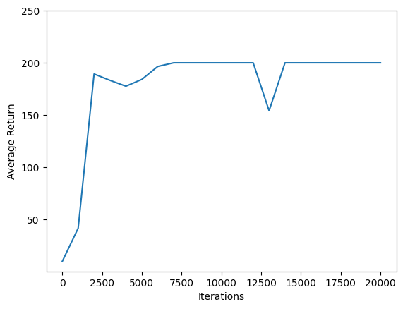
Use matplotlib.pyplot to chart how the policy improved during training.
One iteration of Cartpole-v0 consists of 200 time steps. The environment gives a reward of +1 for each step the pole stays up, so the maximum return for one episode is 200. The charts shows the return increasing towards that maximum each time it is evaluated during training. (It may be a little unstable and not increase monotonically each time.)
iterations = range(0, num_iterations + 1, eval_interval)
plt.plot(iterations, returns)
plt.ylabel('Average Return')
plt.xlabel('Iterations')
plt.ylim(top=250)
(0.08000040054321289, 250.0)
Videos
Charts are nice. But more exciting is seeing an agent actually performing a task in an environment.
First, create a function to embed videos in the notebook.
def embed_mp4(filename):
  """Embeds an mp4 file in the notebook."""
  video = open(filename,'rb').read()
  b64 = base64.b64encode(video)
  tag = '''
  <video width="640" height="480" controls>
    <source src="data:video/mp4;base64,{0}" type="video/mp4">
  Your browser does not support the video tag.
  </video>'''.format(b64.decode())

  return IPython.display.HTML(tag)
Now iterate through a few episodes of the Cartpole game with the agent. The underlying Python environment (the one "inside" the TensorFlow environment wrapper) provides a render() method, which outputs an image of the environment state. These can be collected into a video.
def create_policy_eval_video(policy, filename, num_episodes=5, fps=30):
  filename = filename + ".mp4"
  with imageio.get_writer(filename, fps=fps) as video:
    for _ in range(num_episodes):
      time_step = eval_env.reset()
      video.append_data(eval_py_env.render())
      while not time_step.is_last():
        action_step = policy.action(time_step)
        time_step = eval_env.step(action_step.action)
        video.append_data(eval_py_env.render())
  return embed_mp4(filename)

create_policy_eval_video(agent.policy, "trained-agent")
WARNING:root:IMAGEIO FFMPEG_WRITER WARNING: input image is not divisible by macro_block_size=16, resizing from (400, 600) to (400, 608) to ensure video compatibility with most codecs and players. To prevent resizing, make your input image divisible by the macro_block_size or set the macro_block_size to None (risking incompatibility). You may also see a FFMPEG warning concerning speedloss due to data not being aligned.
[swscaler @ 0x555a5d3cf880] Warning: data is not aligned! This can lead to a speed loss
For fun, compare the trained agent (above) to an agent moving randomly. (It does not do as well.)
create_policy_eval_video(random_policy, "random-agent")
WARNING:root:IMAGEIO FFMPEG_WRITER WARNING: input image is not divisible by macro_block_size=16, resizing from (400, 600) to (400, 608) to ensure video compatibility with most codecs and players. To prevent resizing, make your input image divisible by the macro_block_size or set the macro_block_size to None (risking incompatibility). You may also see a FFMPEG warning concerning speedloss due to data not being aligned.
[swscaler @ 0x55f466934880] Warning: data is not aligned! This can lead to a speed loss