
Copyright 2023 The TF-Agents Authors.
|
|
|
 View source on GitHub
|
|
Introduction
This example shows how to train a Categorical DQN (C51) agent on the Cartpole environment using the TF-Agents library.
Make sure you take a look through the DQN tutorial as a prerequisite. This tutorial will assume familiarity with the DQN tutorial; it will mainly focus on the differences between DQN and C51.
Setup
If you haven't installed tf-agents yet, run:
sudo apt-get updatesudo apt-get install -y xvfb ffmpeg freeglut3-devpip install 'imageio==2.4.0'pip install pyvirtualdisplaypip install tf-agentspip install pygletpip install tf-keras
import os
# Keep using keras-2 (tf-keras) rather than keras-3 (keras).
os.environ['TF_USE_LEGACY_KERAS'] = '1'
from __future__ import absolute_import
from __future__ import division
from __future__ import print_function

import base64
import imageio
import IPython
import matplotlib
import matplotlib.pyplot as plt
import PIL.Image
import pyvirtualdisplay

import tensorflow as tf

from tf_agents.agents.categorical_dqn import categorical_dqn_agent
from tf_agents.drivers import dynamic_step_driver
from tf_agents.environments import suite_gym
from tf_agents.environments import tf_py_environment
from tf_agents.eval import metric_utils
from tf_agents.metrics import tf_metrics
from tf_agents.networks import categorical_q_network
from tf_agents.policies import random_tf_policy
from tf_agents.replay_buffers import tf_uniform_replay_buffer
from tf_agents.trajectories import trajectory
from tf_agents.utils import common

# Set up a virtual display for rendering OpenAI gym environments.
display = pyvirtualdisplay.Display(visible=0, size=(1400, 900)).start()
Hyperparameters
env_name = "CartPole-v1" # @param {type:"string"}
num_iterations = 15000 # @param {type:"integer"}

initial_collect_steps = 1000  # @param {type:"integer"}
collect_steps_per_iteration = 1  # @param {type:"integer"}
replay_buffer_capacity = 100000  # @param {type:"integer"}

fc_layer_params = (100,)

batch_size = 64  # @param {type:"integer"}
learning_rate = 1e-3  # @param {type:"number"}
gamma = 0.99
log_interval = 200  # @param {type:"integer"}

num_atoms = 51  # @param {type:"integer"}
min_q_value = -20  # @param {type:"integer"}
max_q_value = 20  # @param {type:"integer"}
n_step_update = 2  # @param {type:"integer"}

num_eval_episodes = 10  # @param {type:"integer"}
eval_interval = 1000  # @param {type:"integer"}
Environment
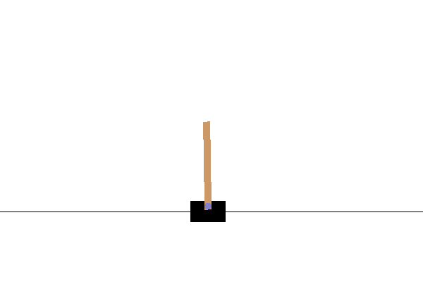
Load the environment as before, with one for training and one for evaluation. Here we use CartPole-v1 (vs. CartPole-v0 in the DQN tutorial), which has a larger max reward of 500 rather than 200.
train_py_env = suite_gym.load(env_name)
eval_py_env = suite_gym.load(env_name)

train_env = tf_py_environment.TFPyEnvironment(train_py_env)
eval_env = tf_py_environment.TFPyEnvironment(eval_py_env)
Agent
C51 is a Q-learning algorithm based on DQN. Like DQN, it can be used on any environment with a discrete action space.
The main difference between C51 and DQN is that rather than simply predicting the Q-value for each state-action pair, C51 predicts a histogram model for the probability distribution of the Q-value:
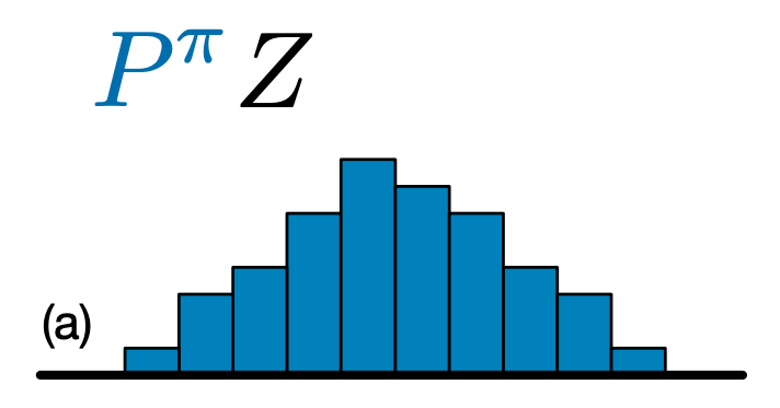
By learning the distribution rather than simply the expected value, the algorithm is able to stay more stable during training, leading to improved final performance. This is particularly true in situations with bimodal or even multimodal value distributions, where a single average does not provide an accurate picture.
In order to train on probability distributions rather than on values, C51 must perform some complex distributional computations in order to calculate its loss function. But don't worry, all of this is taken care of for you in TF-Agents!
To create a C51 Agent, we first need to create a CategoricalQNetwork. The API of the CategoricalQNetwork is the same as that of the QNetwork, except that there is an additional argument num_atoms. This represents the number of support points in our probability distribution estimates. (The above image includes 10 support points, each represented by a vertical blue bar.) As you can tell from the name, the default number of atoms is 51.
categorical_q_net = categorical_q_network.CategoricalQNetwork(
    train_env.observation_spec(),
    train_env.action_spec(),
    num_atoms=num_atoms,
    fc_layer_params=fc_layer_params)
We also need an optimizer to train the network we just created, and a train_step_counter variable to keep track of how many times the network was updated.
Note that one other significant difference from vanilla DqnAgent is that we now need to specify min_q_value and max_q_value as arguments. These specify the most extreme values of the support (in other words, the most extreme of the 51 atoms on either side). Make sure to choose these appropriately for your particular environment. Here we use -20 and 20.
optimizer = tf.compat.v1.train.AdamOptimizer(learning_rate=learning_rate)

train_step_counter = tf.Variable(0)

agent = categorical_dqn_agent.CategoricalDqnAgent(
    train_env.time_step_spec(),
    train_env.action_spec(),
    categorical_q_network=categorical_q_net,
    optimizer=optimizer,
    min_q_value=min_q_value,
    max_q_value=max_q_value,
    n_step_update=n_step_update,
    td_errors_loss_fn=common.element_wise_squared_loss,
    gamma=gamma,
    train_step_counter=train_step_counter)
agent.initialize()
One last thing to note is that we also added an argument to use n-step updates with \(n\) = 2. In single-step Q-learning (\(n\) = 1), we only compute the error between the Q-values at the current time step and the next time step using the single-step return (based on the Bellman optimality equation). The single-step return is defined as:
\(G_t = R_{t + 1} + \gamma V(s_{t + 1})\)
where we define \(V(s) = \max_a{Q(s, a)}\).
N-step updates involve expanding the standard single-step return function \(n\) times:
\(G_t^n = R_{t + 1} + \gamma R_{t + 2} + \gamma^2 R_{t + 3} + \dots + \gamma^n V(s_{t + n})\)
N-step updates enable the agent to bootstrap from further in the future, and with the right value of \(n\), this often leads to faster learning.
Although C51 and n-step updates are often combined with prioritized replay to form the core of the Rainbow agent, we saw no measurable improvement from implementing prioritized replay. Moreover, we find that when combining our C51 agent with n-step updates alone, our agent performs as well as other Rainbow agents on the sample of Atari environments we've tested.
Metrics and Evaluation
The most common metric used to evaluate a policy is the average return. The return is the sum of rewards obtained while running a policy in an environment for an episode, and we usually average this over a few episodes. We can compute the average return metric as follows.
def compute_avg_return(environment, policy, num_episodes=10):

  total_return = 0.0
  for _ in range(num_episodes):

    time_step = environment.reset()
    episode_return = 0.0

    while not time_step.is_last():
      action_step = policy.action(time_step)
      time_step = environment.step(action_step.action)
      episode_return += time_step.reward
    total_return += episode_return

  avg_return = total_return / num_episodes
  return avg_return.numpy()[0]


random_policy = random_tf_policy.RandomTFPolicy(train_env.time_step_spec(),
                                                train_env.action_spec())

compute_avg_return(eval_env, random_policy, num_eval_episodes)

# Please also see the metrics module for standard implementations of different
# metrics.
37.7
Data Collection
As in the DQN tutorial, set up the replay buffer and the initial data collection with the random policy.
replay_buffer = tf_uniform_replay_buffer.TFUniformReplayBuffer(
    data_spec=agent.collect_data_spec,
    batch_size=train_env.batch_size,
    max_length=replay_buffer_capacity)

def collect_step(environment, policy):
  time_step = environment.current_time_step()
  action_step = policy.action(time_step)
  next_time_step = environment.step(action_step.action)
  traj = trajectory.from_transition(time_step, action_step, next_time_step)

  # Add trajectory to the replay buffer
  replay_buffer.add_batch(traj)

for _ in range(initial_collect_steps):
  collect_step(train_env, random_policy)

# This loop is so common in RL, that we provide standard implementations of
# these. For more details see the drivers module.

# Dataset generates trajectories with shape [BxTx...] where
# T = n_step_update + 1.
dataset = replay_buffer.as_dataset(
    num_parallel_calls=3, sample_batch_size=batch_size,
    num_steps=n_step_update + 1).prefetch(3)

iterator = iter(dataset)
WARNING:tensorflow:From /tmpfs/src/tf_docs_env/lib/python3.9/site-packages/tensorflow/python/autograph/impl/api.py:377: ReplayBuffer.get_next (from tf_agents.replay_buffers.replay_buffer) is deprecated and will be removed in a future version.
Instructions for updating:
Use `as_dataset(..., single_deterministic_pass=False) instead.
Training the agent
The training loop involves both collecting data from the environment and optimizing the agent's networks. Along the way, we will occasionally evaluate the agent's policy to see how we are doing.
The following will take ~7 minutes to run.
try:
  %%time
except:
  pass

# (Optional) Optimize by wrapping some of the code in a graph using TF function.
agent.train = common.function(agent.train)

# Reset the train step
agent.train_step_counter.assign(0)

# Evaluate the agent's policy once before training.
avg_return = compute_avg_return(eval_env, agent.policy, num_eval_episodes)
returns = [avg_return]

for _ in range(num_iterations):

  # Collect a few steps using collect_policy and save to the replay buffer.
  for _ in range(collect_steps_per_iteration):
    collect_step(train_env, agent.collect_policy)

  # Sample a batch of data from the buffer and update the agent's network.
  experience, unused_info = next(iterator)
  train_loss = agent.train(experience)

  step = agent.train_step_counter.numpy()

  if step % log_interval == 0:
    print('step = {0}: loss = {1}'.format(step, train_loss.loss))

  if step % eval_interval == 0:
    avg_return = compute_avg_return(eval_env, agent.policy, num_eval_episodes)
    print('step = {0}: Average Return = {1:.2f}'.format(step, avg_return))
    returns.append(avg_return)
WARNING:tensorflow:From /tmpfs/src/tf_docs_env/lib/python3.9/site-packages/tensorflow/python/util/dispatch.py:1260: calling foldr_v2 (from tensorflow.python.ops.functional_ops) with back_prop=False is deprecated and will be removed in a future version.
Instructions for updating:
back_prop=False is deprecated. Consider using tf.stop_gradient instead.
Instead of:
results = tf.foldr(fn, elems, back_prop=False)
Use:
results = tf.nest.map_structure(tf.stop_gradient, tf.foldr(fn, elems))
step = 200: loss = 3.2159409523010254
step = 400: loss = 2.422974109649658
step = 600: loss = 1.9803032875061035
step = 800: loss = 1.733839750289917
step = 1000: loss = 1.705157995223999
step = 1000: Average Return = 88.60
step = 1200: loss = 1.655350923538208
step = 1400: loss = 1.419114351272583
step = 1600: loss = 1.2578476667404175
step = 1800: loss = 1.3189895153045654
step = 2000: loss = 0.9676651954650879
step = 2000: Average Return = 130.80
step = 2200: loss = 0.7909003496170044
step = 2400: loss = 0.9291537404060364
step = 2600: loss = 0.8300429582595825
step = 2800: loss = 0.9739845991134644
step = 3000: loss = 0.5435967445373535
step = 3000: Average Return = 261.40
step = 3200: loss = 0.7065144777297974
step = 3400: loss = 0.8492055535316467
step = 3600: loss = 0.808651864528656
step = 3800: loss = 0.48259130120277405
step = 4000: loss = 0.9187874794006348
step = 4000: Average Return = 280.90
step = 4200: loss = 0.7415772676467896
step = 4400: loss = 0.621947169303894
step = 4600: loss = 0.5226543545722961
step = 4800: loss = 0.7011302709579468
step = 5000: loss = 0.7732619047164917
step = 5000: Average Return = 271.70
step = 5200: loss = 0.8493011593818665
step = 5400: loss = 0.6786139011383057
step = 5600: loss = 0.5639233589172363
step = 5800: loss = 0.48468759655952454
step = 6000: loss = 0.6366198062896729
step = 6000: Average Return = 350.70
step = 6200: loss = 0.4855012893676758
step = 6400: loss = 0.4458327889442444
step = 6600: loss = 0.6745614409446716
step = 6800: loss = 0.5021890997886658
step = 7000: loss = 0.4639193117618561
step = 7000: Average Return = 343.00
step = 7200: loss = 0.4711253345012665
step = 7400: loss = 0.5891958475112915
step = 7600: loss = 0.3957907557487488
step = 7800: loss = 0.4868921637535095
step = 8000: loss = 0.5140666365623474
step = 8000: Average Return = 396.10
step = 8200: loss = 0.6051771640777588
step = 8400: loss = 0.6179391741752625
step = 8600: loss = 0.5253893733024597
step = 8800: loss = 0.3697047531604767
step = 9000: loss = 0.7271263599395752
step = 9000: Average Return = 320.20
step = 9200: loss = 0.5285177826881409
step = 9400: loss = 0.4590812921524048
step = 9600: loss = 0.4743385910987854
step = 9800: loss = 0.47938746213912964
step = 10000: loss = 0.5290409326553345
step = 10000: Average Return = 433.00
step = 10200: loss = 0.4573556184768677
step = 10400: loss = 0.352144718170166
step = 10600: loss = 0.39160820841789246
step = 10800: loss = 0.3254846930503845
step = 11000: loss = 0.37145161628723145
step = 11000: Average Return = 414.60
step = 11200: loss = 0.382583349943161
step = 11400: loss = 0.44465434551239014
step = 11600: loss = 0.4484185576438904
step = 11800: loss = 0.248131662607193
step = 12000: loss = 0.5516679883003235
step = 12000: Average Return = 375.40
step = 12200: loss = 0.3307253420352936
step = 12400: loss = 0.19486135244369507
step = 12600: loss = 0.31668007373809814
step = 12800: loss = 0.4462052285671234
step = 13000: loss = 0.241848886013031
step = 13000: Average Return = 326.80
step = 13200: loss = 0.20919030904769897
step = 13400: loss = 0.2044396996498108
step = 13600: loss = 0.428558886051178
step = 13800: loss = 0.1880824714899063
step = 14000: loss = 0.34256821870803833
step = 14000: Average Return = 345.50
step = 14200: loss = 0.22452744841575623
step = 14400: loss = 0.29694461822509766
step = 14600: loss = 0.4149337410926819
step = 14800: loss = 0.41922691464424133
step = 15000: loss = 0.4064670205116272
step = 15000: Average Return = 242.10
Visualization
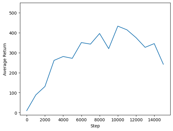
Plots
We can plot return vs global steps to see the performance of our agent. In Cartpole-v1, the environment gives a reward of +1 for every time step the pole stays up, and since the maximum number of steps is 500, the maximum possible return is also 500.
steps = range(0, num_iterations + 1, eval_interval)
plt.plot(steps, returns)
plt.ylabel('Average Return')
plt.xlabel('Step')
plt.ylim(top=550)
(-11.255000400543214, 550.0)
Videos
It is helpful to visualize the performance of an agent by rendering the environment at each step. Before we do that, let us first create a function to embed videos in this colab.
def embed_mp4(filename):
  """Embeds an mp4 file in the notebook."""
  video = open(filename,'rb').read()
  b64 = base64.b64encode(video)
  tag = '''
  <video width="640" height="480" controls>
    <source src="data:video/mp4;base64,{0}" type="video/mp4">
  Your browser does not support the video tag.
  </video>'''.format(b64.decode())

  return IPython.display.HTML(tag)
The following code visualizes the agent's policy for a few episodes:
num_episodes = 3
video_filename = 'imageio.mp4'
with imageio.get_writer(video_filename, fps=60) as video:
  for _ in range(num_episodes):
    time_step = eval_env.reset()
    video.append_data(eval_py_env.render())
    while not time_step.is_last():
      action_step = agent.policy.action(time_step)
      time_step = eval_env.step(action_step.action)
      video.append_data(eval_py_env.render())

embed_mp4(video_filename)
WARNING:root:IMAGEIO FFMPEG_WRITER WARNING: input image is not divisible by macro_block_size=16, resizing from (400, 600) to (400, 608) to ensure video compatibility with most codecs and players. To prevent resizing, make your input image divisible by the macro_block_size or set the macro_block_size to None (risking incompatibility). You may also see a FFMPEG warning concerning speedloss due to data not being aligned.
[swscaler @ 0x55f48c41d880] Warning: data is not aligned! This can lead to a speed loss
C51 tends to do slightly better than DQN on CartPole-v1, but the difference between the two agents becomes more and more significant in increasingly complex environments. For example, on the full Atari 2600 benchmark, C51 demonstrates a mean score improvement of 126% over DQN after normalizing with respect to a random agent. Additional improvements can be gained by including n-step updates.
For a deeper dive into the C51 algorithm, see A Distributional Perspective on Reinforcement Learning (2017).