|
|
|
 View source on GitHub View source on GitHub
|
|
Overview
This tutorial is an overview of the constraints and regularizers provided by the TensorFlow Lattice (TFL) library. Here we use TFL premade models on synthetic datasets, but note that everything in this tutorial can also be done with models constructed from TFL Keras layers.
Before proceeding, make sure your runtime has all required packages installed (as imported in the code cells below).
Setup
Installing TF Lattice package:
pip install -U tensorflow tf-keras tensorflow-lattice pydot graphvizpip install -U tensorflow_decision_forests
Importing required packages:
import tensorflow as tf
import tensorflow_lattice as tfl
import tensorflow_decision_forests as tfdf

from IPython.core.pylabtools import figsize
import functools
import logging
import matplotlib
from matplotlib import pyplot as plt
import numpy as np
import pandas as pd
import sys
import tempfile
logging.disable(sys.maxsize)
2026-03-06 12:18:48.778615: E external/local_xla/xla/stream_executor/cuda/cuda_fft.cc:467] Unable to register cuFFT factory: Attempting to register factory for plugin cuFFT when one has already been registered
WARNING: All log messages before absl::InitializeLog() is called are written to STDERR
E0000 00:00:1772799528.801679   11080 cuda_dnn.cc:8579] Unable to register cuDNN factory: Attempting to register factory for plugin cuDNN when one has already been registered
E0000 00:00:1772799528.809523   11080 cuda_blas.cc:1407] Unable to register cuBLAS factory: Attempting to register factory for plugin cuBLAS when one has already been registered
W0000 00:00:1772799528.828320   11080 computation_placer.cc:177] computation placer already registered. Please check linkage and avoid linking the same target more than once.
W0000 00:00:1772799528.828339   11080 computation_placer.cc:177] computation placer already registered. Please check linkage and avoid linking the same target more than once.
W0000 00:00:1772799528.828341   11080 computation_placer.cc:177] computation placer already registered. Please check linkage and avoid linking the same target more than once.
W0000 00:00:1772799528.828344   11080 computation_placer.cc:177] computation placer already registered. Please check linkage and avoid linking the same target more than once.
# Use Keras 2.
version_fn = getattr(tf.keras, "version", None)
if version_fn and version_fn().startswith("3."):
  import tf_keras as keras
else:
  keras = tf.keras
Default values used in this guide:
NUM_EPOCHS = 1000
BATCH_SIZE = 64
LEARNING_RATE=0.01
Training Dataset for Ranking Restaurants
Imagine a simplified scenario where we want to determine whether or not users will click on a restaurant search result. The task is to predict the clickthrough rate (CTR) given input features:
- Average rating (
avg_rating): a numeric feature with values in the range [1,5]. - Number of reviews (
num_reviews): a numeric feature with values capped at 200, which we use as a measure of trendiness. - Dollar rating (
dollar_rating): a categorical feature with string values in the set {"D", "DD", "DDD", "DDDD"}.
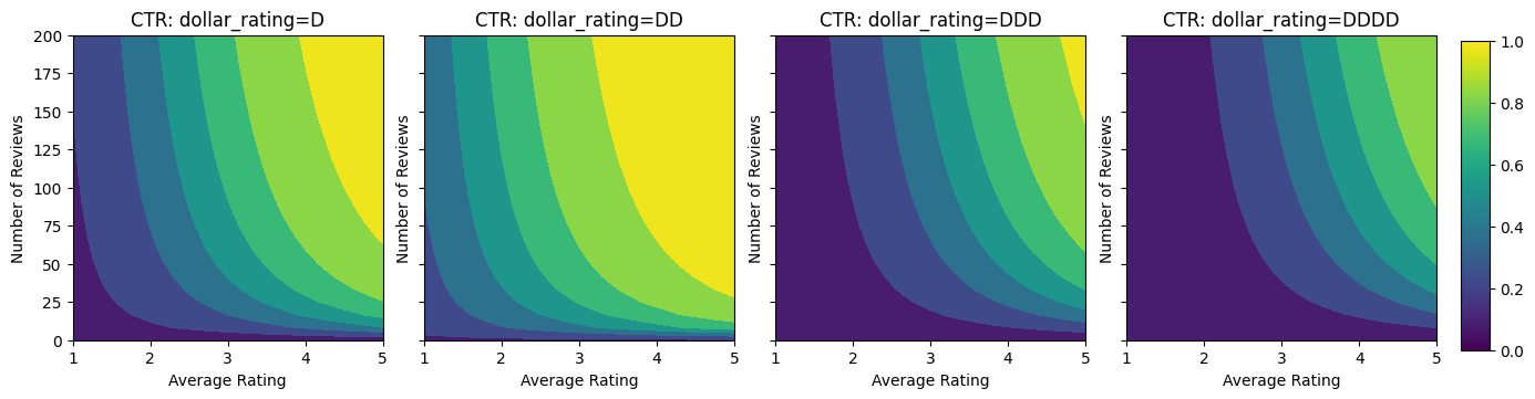
Here we create a synthetic dataset where the true CTR is given by the formula:
\[ CTR = 1 / (1 + exp\{\mbox{b(dollar_rating)}-\mbox{avg_rating}\times log(\mbox{num_reviews}) /4 \}) \]
where \(b(\cdot)\) translates each dollar_rating to a baseline value:
\[ \mbox{D}\to 3,\ \mbox{DD}\to 2,\ \mbox{DDD}\to 4,\ \mbox{DDDD}\to 4.5. \]
This formula reflects typical user patterns. e.g. given everything else fixed, users prefer restaurants with higher star ratings, and "\$\$" restaurants will receive more clicks than "\$", followed by "\$\$\$" and "\$\$\$\$".
dollar_ratings_vocab = ["D", "DD", "DDD", "DDDD"]
def click_through_rate(avg_ratings, num_reviews, dollar_ratings):
  dollar_rating_baseline = {"D": 3, "DD": 2, "DDD": 4, "DDDD": 4.5}
  return 1 / (1 + np.exp(
      np.array([dollar_rating_baseline[d] for d in dollar_ratings]) -
      avg_ratings * np.log1p(num_reviews) / 4))
Let's take a look at the contour plots of this CTR function.
def color_bar():
  bar = matplotlib.cm.ScalarMappable(
      norm=matplotlib.colors.Normalize(0, 1, True),
      cmap="viridis",
  )
  bar.set_array([0, 1])
  return bar


def plot_fns(fns, res=25):
  """Generates contour plots for a list of (name, fn) functions."""
  num_reviews, avg_ratings = np.meshgrid(
      np.linspace(0, 200, num=res),
      np.linspace(1, 5, num=res),
  )
  figsize(13, 3.5 * len(fns))
  fig, axes = plt.subplots(
      len(fns), len(dollar_ratings_vocab), sharey=True, layout="constrained"
  )
  axes = axes.flatten()
  axes_index = 0
  for fn_name, fn in fns:
    for dollar_rating_split in dollar_ratings_vocab:
      dollar_ratings = np.repeat(dollar_rating_split, res**2)
      values = fn(avg_ratings.flatten(), num_reviews.flatten(), dollar_ratings)
      title = "{}: dollar_rating={}".format(fn_name, dollar_rating_split)
      subplot = axes[axes_index]
      axes_index += 1
      subplot.contourf(
          avg_ratings,
          num_reviews,
          np.reshape(values, (res, res)),
          vmin=0,
          vmax=1,
      )
      subplot.title.set_text(title)
      subplot.set(xlabel="Average Rating")
      subplot.set(ylabel="Number of Reviews")
      subplot.set(xlim=(1, 5))

  if len(fns) <= 2:
    cax = fig.add_axes([
        axes[-1].get_position().x1 + 0.11,
        axes[-1].get_position().y0,
        0.02,
        0.8,
    ])
    _ = fig.colorbar(color_bar(), cax=cax)


plot_fns([("CTR", click_through_rate)])
Preparing Data
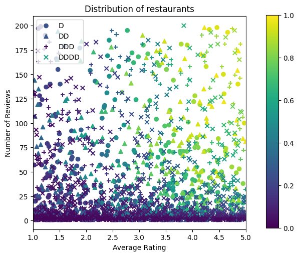
We now need to create our synthetic datasets. We start by generating a simulated dataset of restaurants and their features.
def sample_restaurants(n):
  avg_ratings = np.random.uniform(1.0, 5.0, n)
  num_reviews = np.round(np.exp(np.random.uniform(0.0, np.log(200), n)))
  dollar_ratings = np.random.choice(dollar_ratings_vocab, n)
  ctr_labels = click_through_rate(avg_ratings, num_reviews, dollar_ratings)
  return avg_ratings, num_reviews, dollar_ratings, ctr_labels


np.random.seed(42)
avg_ratings, num_reviews, dollar_ratings, ctr_labels = sample_restaurants(2000)

figsize(5, 5)
fig, axs = plt.subplots(1, 1, sharey=False, layout="constrained")

for rating, marker in [("D", "o"), ("DD", "^"), ("DDD", "+"), ("DDDD", "x")]:
  plt.scatter(
      x=avg_ratings[np.where(dollar_ratings == rating)],
      y=num_reviews[np.where(dollar_ratings == rating)],
      c=ctr_labels[np.where(dollar_ratings == rating)],
      vmin=0,
      vmax=1,
      marker=marker,
      label=rating)
plt.xlabel("Average Rating")
plt.ylabel("Number of Reviews")
plt.legend()
plt.xlim((1, 5))
plt.title("Distribution of restaurants")
_ = fig.colorbar(color_bar(), cax=fig.add_axes([1.05, 0.1, 0.05, 0.85]))
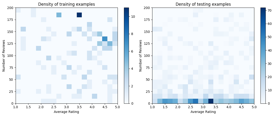
Let's produce the training, validation and testing datasets. When a restaurant is viewed in the search results, we can record user's engagement (click or no click) as a sample point.
In practice, users often do not go through all search results. This means that users will likely only see restaurants already considered "good" by the current ranking model in use. As a result, "good" restaurants are more frequently impressed and over-represented in the training datasets. When using more features, the training dataset can have large gaps in "bad" parts of the feature space.
When the model is used for ranking, it is often evaluated on all relevant results with a more uniform distribution that is not well-represented by the training dataset. A flexible and complicated model might fail in this case due to overfitting the over-represented data points and thus lack generalizability. We handle this issue by applying domain knowledge to add shape constraints that guide the model to make reasonable predictions when it cannot pick them up from the training dataset.
In this example, the training dataset mostly consists of user interactions with good and popular restaurants. The testing dataset has a uniform distribution to simulate the evaluation setting discussed above. Note that such testing dataset will not be available in a real problem setting.
def sample_dataset(n, testing_set):
  (avg_ratings, num_reviews, dollar_ratings, ctr_labels) = sample_restaurants(n)
  if testing_set:
    # Testing has a more uniform distribution over all restaurants.
    num_views = np.random.poisson(lam=3, size=n)
  else:
    # Training/validation datasets have more views on popular restaurants.
    num_views = np.random.poisson(lam=ctr_labels * num_reviews / 50.0, size=n)

  return pd.DataFrame({
      "avg_rating": np.repeat(avg_ratings, num_views),
      "num_reviews": np.repeat(num_reviews, num_views),
      "dollar_rating": np.repeat(dollar_ratings, num_views),
      "clicked": np.random.binomial(n=1, p=np.repeat(ctr_labels, num_views)),
  })


# Generate datasets.
np.random.seed(42)
data_train = sample_dataset(500, testing_set=False)
data_val = sample_dataset(500, testing_set=False)
data_test = sample_dataset(500, testing_set=True)

ds_train = tfdf.keras.pd_dataframe_to_tf_dataset(
    data_train, label="clicked", batch_size=BATCH_SIZE
)
ds_val = tfdf.keras.pd_dataframe_to_tf_dataset(
    data_val, label="clicked", batch_size=BATCH_SIZE
)
ds_test = tfdf.keras.pd_dataframe_to_tf_dataset(
    data_test, label="clicked", batch_size=BATCH_SIZE
)

# feature_analysis_data is used to find quantiles of featurse.
feature_analysis_data = data_train.copy()
feature_analysis_data["dollar_rating"] = feature_analysis_data[
    "dollar_rating"
].map({v: i for i, v in enumerate(dollar_ratings_vocab)})
feature_analysis_data = dict(feature_analysis_data)

# Plotting dataset densities.
figsize(12, 5)
fig, axs = plt.subplots(1, 2, sharey=False, tight_layout=False)
for ax, data, title in [
    (axs[0], data_train, "training"),
    (axs[1], data_test, "testing"),
]:
  _, _, _, density = ax.hist2d(
      x=data["avg_rating"],
      y=data["num_reviews"],
      bins=(np.linspace(1, 5, num=21), np.linspace(0, 200, num=21)),
      cmap="Blues",
  )
  ax.set(xlim=(1, 5))
  ax.set(ylim=(0, 200))
  ax.set(xlabel="Average Rating")
  ax.set(ylabel="Number of Reviews")
  ax.title.set_text("Density of {} examples".format(title))
  _ = fig.colorbar(density, ax=ax)
2026-03-06 12:18:53.251901: E external/local_xla/xla/stream_executor/cuda/cuda_platform.cc:51] failed call to cuInit: INTERNAL: CUDA error: Failed call to cuInit: CUDA_ERROR_NO_DEVICE: no CUDA-capable device is detected
Fitting Gradient Boosted Trees
We first create a few auxillary functions for plotting and calculating validation and test metrics.
def pred_fn(model, from_logits, avg_ratings, num_reviews, dollar_rating):
  preds = model.predict(
      tf.data.Dataset.from_tensor_slices({
          "avg_rating": avg_ratings,
          "num_reviews": num_reviews,
          "dollar_rating": dollar_rating,
      }).batch(1),
      verbose=0,
  )
  if from_logits:
    preds = tf.math.sigmoid(preds)
  return preds


def analyze_model(models, from_logits=False, print_metrics=True):
  pred_fns = []
  for model, name in models:
    if print_metrics:
      metric = model.evaluate(ds_val, return_dict=True, verbose=0)
      print("Validation AUC: {}".format(metric["auc"]))
      metric = model.evaluate(ds_test, return_dict=True, verbose=0)
      print("Testing AUC: {}".format(metric["auc"]))

    pred_fns.append(
        ("{} pCTR".format(name), functools.partial(pred_fn, model, from_logits))
    )

  pred_fns.append(("CTR", click_through_rate))
  plot_fns(pred_fns)
We can fit TensorFlow gradient boosted decision trees on the dataset:
gbt_model = tfdf.keras.GradientBoostedTreesModel(
    features=[
        tfdf.keras.FeatureUsage(name="num_reviews"),
        tfdf.keras.FeatureUsage(name="avg_rating"),
        tfdf.keras.FeatureUsage(name="dollar_rating"),
    ],
    exclude_non_specified_features=True,
    num_threads=1,
    num_trees=32,
    max_depth=6,
    min_examples=10,
    growing_strategy="BEST_FIRST_GLOBAL",
    random_seed=42,
    temp_directory=tempfile.mkdtemp(),
)
gbt_model.compile(metrics=[keras.metrics.AUC(name="auc")])
gbt_model.fit(ds_train, validation_data=ds_val, verbose=0)
analyze_model([(gbt_model, "GBT")])
WARNING: All log messages before absl::InitializeLog() is called are written to STDERR
W0000 00:00:1772799533.967485   11080 gradient_boosted_trees.cc:1873] "goss_alpha" set but "sampling_method" not equal to "GOSS".
W0000 00:00:1772799533.967547   11080 gradient_boosted_trees.cc:1883] "goss_beta" set but "sampling_method" not equal to "GOSS".
W0000 00:00:1772799533.967551   11080 gradient_boosted_trees.cc:1897] "selective_gradient_boosting_ratio" set but "sampling_method" not equal to "SELGB".
Num validation examples: tf.Tensor(155, shape=(), dtype=int32)
I0000 00:00:1772799537.814615   11080 kernel.cc:782] Start Yggdrasil model training
I0000 00:00:1772799537.814653   11080 kernel.cc:783] Collect training examples
I0000 00:00:1772799537.814663   11080 kernel.cc:795] Dataspec guide:
column_guides {
  column_name_pattern: "^__LABEL$"
  type: CATEGORICAL
  categorial {
    min_vocab_frequency: 0
    max_vocab_count: -1
  }
}
column_guides {
  column_name_pattern: "^num_reviews$"
}
column_guides {
  column_name_pattern: "^avg_rating$"
}
column_guides {
  column_name_pattern: "^dollar_rating$"
}
default_column_guide {
  categorial {
    max_vocab_count: 2000
  }
  discretized_numerical {
    maximum_num_bins: 255
  }
}
ignore_columns_without_guides: true
detect_numerical_as_discretized_numerical: false

I0000 00:00:1772799537.815112   11080 kernel.cc:401] Number of batches: 3
I0000 00:00:1772799537.815123   11080 kernel.cc:402] Number of examples: 162
I0000 00:00:1772799537.815179   11080 kernel.cc:802] Training dataset:
Number of records: 162
Number of columns: 4

Number of columns by type:
    CATEGORICAL: 2 (50%)
    NUMERICAL: 2 (50%)

Columns:

CATEGORICAL: 2 (50%)
    0: "__LABEL" CATEGORICAL integerized vocab-size:3 no-ood-item
    2: "dollar_rating" CATEGORICAL has-dict vocab-size:5 zero-ood-items most-frequent:"D" 61 (37.6543%)

NUMERICAL: 2 (50%)
    1: "avg_rating" NUMERICAL mean:3.52831 min:1.14939 max:4.90341 sd:1.04368
    3: "num_reviews" NUMERICAL mean:107.932 min:6 max:200 sd:52.6472

Terminology:
    nas: Number of non-available (i.e. missing) values.
    ood: Out of dictionary.
    manually-defined: Attribute whose type is manually defined by the user, i.e., the type was not automatically inferred.
    tokenized: The attribute value is obtained through tokenization.
    has-dict: The attribute is attached to a string dictionary e.g. a categorical attribute stored as a string.
    vocab-size: Number of unique values.

I0000 00:00:1772799537.815200   11080 kernel.cc:807] Collect validation dataset
I0000 00:00:1772799537.815235   11080 kernel.cc:401] Number of batches: 3
I0000 00:00:1772799537.815238   11080 kernel.cc:402] Number of examples: 155
I0000 00:00:1772799537.815266   11080 kernel.cc:813] Validation dataset:
Number of records: 155
Number of columns: 4

Number of columns by type:
    CATEGORICAL: 2 (50%)
    NUMERICAL: 2 (50%)

Columns:

CATEGORICAL: 2 (50%)
    0: "__LABEL" CATEGORICAL integerized vocab-size:3 no-ood-item
    2: "dollar_rating" CATEGORICAL has-dict vocab-size:5 zero-ood-items most-frequent:"D" 55 (35.4839%)

NUMERICAL: 2 (50%)
    1: "avg_rating" NUMERICAL mean:3.58594 min:1.11015 max:4.99128 sd:1.03425
    3: "num_reviews" NUMERICAL mean:103.374 min:8 max:195 sd:54.6089

Terminology:
    nas: Number of non-available (i.e. missing) values.
    ood: Out of dictionary.
    manually-defined: Attribute whose type is manually defined by the user, i.e., the type was not automatically inferred.
    tokenized: The attribute value is obtained through tokenization.
    has-dict: The attribute is attached to a string dictionary e.g. a categorical attribute stored as a string.
    vocab-size: Number of unique values.

I0000 00:00:1772799537.815278   11080 kernel.cc:818] Configure learner
W0000 00:00:1772799537.815475   11080 gradient_boosted_trees.cc:1873] "goss_alpha" set but "sampling_method" not equal to "GOSS".
W0000 00:00:1772799537.815484   11080 gradient_boosted_trees.cc:1883] "goss_beta" set but "sampling_method" not equal to "GOSS".
W0000 00:00:1772799537.815487   11080 gradient_boosted_trees.cc:1897] "selective_gradient_boosting_ratio" set but "sampling_method" not equal to "SELGB".
I0000 00:00:1772799537.815525   11080 kernel.cc:831] Training config:
learner: "GRADIENT_BOOSTED_TREES"
features: "^avg_rating$"
features: "^dollar_rating$"
features: "^num_reviews$"
label: "^__LABEL$"
task: CLASSIFICATION
random_seed: 42
metadata {
  framework: "TF Keras"
}
pure_serving_model: false
[yggdrasil_decision_forests.model.gradient_boosted_trees.proto.gradient_boosted_trees_config] {
  num_trees: 32
  decision_tree {
    max_depth: 6
    min_examples: 10
    in_split_min_examples_check: true
    keep_non_leaf_label_distribution: true
    num_candidate_attributes: -1
    missing_value_policy: GLOBAL_IMPUTATION
    allow_na_conditions: false
    categorical_set_greedy_forward {
      sampling: 0.1
      max_num_items: -1
      min_item_frequency: 1
    }
    growing_strategy_best_first_global {
    }
    categorical {
      cart {
      }
    }
    axis_aligned_split {
    }
    internal {
      sorting_strategy: PRESORTED
    }
    uplift {
      min_examples_in_treatment: 5
      split_score: KULLBACK_LEIBLER
    }
    numerical_vector_sequence {
      max_num_test_examples: 1000
      num_random_selected_anchors: 100
    }
  }
  shrinkage: 0.1
  loss: DEFAULT
  validation_set_ratio: 0.1
  validation_interval_in_trees: 1
  early_stopping: VALIDATION_LOSS_INCREASE
  early_stopping_num_trees_look_ahead: 30
  l2_regularization: 0
  lambda_loss: 1
  mart {
  }
  adapt_subsample_for_maximum_training_duration: false
  l1_regularization: 0
  use_hessian_gain: false
  l2_regularization_categorical: 1
  xe_ndcg {
    ndcg_truncation: 5
  }
  stochastic_gradient_boosting {
    ratio: 1
  }
  apply_link_function: true
  compute_permutation_variable_importance: false
  early_stopping_initial_iteration: 10
}

I0000 00:00:1772799537.815834   11080 kernel.cc:834] Deployment config:
cache_path: "/tmpfs/tmp/tmpyvfgudk4/working_cache"
num_threads: 1
try_resume_training: true

I0000 00:00:1772799537.816033   11317 kernel.cc:895] Train model
I0000 00:00:1772799537.816130   11317 gradient_boosted_trees.cc:577] Default loss set to BINOMIAL_LOG_LIKELIHOOD
I0000 00:00:1772799537.816150   11317 gradient_boosted_trees.cc:1190] Training gradient boosted tree on 162 example(s) and 3 feature(s).
I0000 00:00:1772799537.816191   11317 gradient_boosted_trees.cc:1230] 162 examples used for training and 155 examples used for validation
I0000 00:00:1772799537.816415   11317 gpu.cc:93] Cannot initialize GPU: Not compiled with GPU support
I0000 00:00:1772799537.816944   11317 gradient_boosted_trees.cc:1632] Train tree 1/32 train-loss:1.170409 train-accuracy:0.691358 valid-loss:1.253763 valid-accuracy:0.664516 [total:0.00s iter:0.00s]
I0000 00:00:1772799537.817043   11317 gradient_boosted_trees.cc:1632] Train tree 2/32 train-loss:1.114586 train-accuracy:0.691358 valid-loss:1.226951 valid-accuracy:0.664516 [total:0.00s iter:0.00s]
I0000 00:00:1772799537.820366   11317 gradient_boosted_trees.cc:1634] Train tree 3/32 train-loss:1.067780 train-accuracy:0.691358 valid-loss:1.213493 valid-accuracy:0.664516 [total:0.00s iter:0.00s]
I0000 00:00:1772799537.823322   11317 gradient_boosted_trees.cc:1632] Train tree 32/32 train-loss:0.619268 train-accuracy:0.870370 valid-loss:1.215939 valid-accuracy:0.690323 [total:0.01s iter:0.00s]
I0000 00:00:1772799537.823341   11317 gradient_boosted_trees.cc:1669] Create final snapshot of the model at iteration 32
I0000 00:00:1772799537.824386   11317 gradient_boosted_trees.cc:279] Truncates the model to 21 tree(s) i.e. 21  iteration(s).
I0000 00:00:1772799537.824445   11317 gradient_boosted_trees.cc:341] Final model num-trees:21 valid-loss:1.160601 valid-accuracy:0.677419
I0000 00:00:1772799537.824684   11317 kernel.cc:926] Export model in log directory: /tmpfs/tmp/tmpyvfgudk4 with prefix a8c03a7a1da445b6
I0000 00:00:1772799537.825221   11317 kernel.cc:944] Save model in resources
I0000 00:00:1772799537.826674   11080 abstract_model.cc:921] Model self evaluation:
Task: CLASSIFICATION
Label: __LABEL
Loss (BINOMIAL_LOG_LIKELIHOOD): 1.1606

Accuracy: 0.677419  CI95[W][0 1]
ErrorRate: : 0.322581


Confusion Table:
truth\prediction
    1   2
1  16  36
2  14  89
Total: 155


WARNING: All log messages before absl::InitializeLog() is called are written to STDERR
I0000 00:00:1772799537.838553   11080 quick_scorer_extended.cc:927] The binary was compiled without AVX2 support, but your CPU supports it. Enable it for faster model inference.
I0000 00:00:1772799537.838675   11080 abstract_model.cc:1439] Engine "GradientBoostedTreesQuickScorerExtended" built
Validation AUC: 0.7145258188247681
Testing AUC: 0.8356180191040039
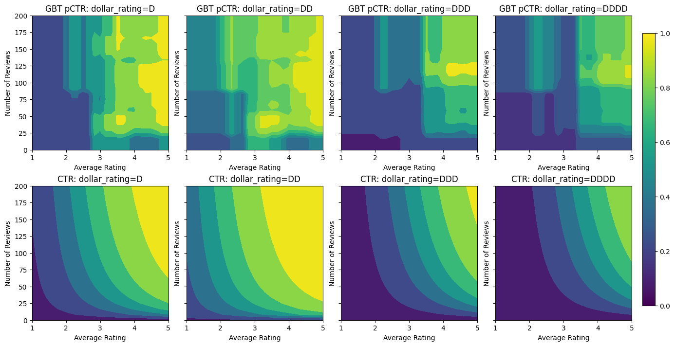
Even though the model has captured the general shape of the true CTR and has decent validation metrics, it has counter-intuitive behavior in several parts of the input space: the estimated CTR decreases as the average rating or number of reviews increase. This is due to a lack of sample points in areas not well-covered by the training dataset. The model simply has no way to deduce the correct behaviour solely from the data.
To solve this issue, we enforce the shape constraint that the model must output values monotonically increasing with respect to both the average rating and the number of reviews. We will later see how to implement this in TFL.
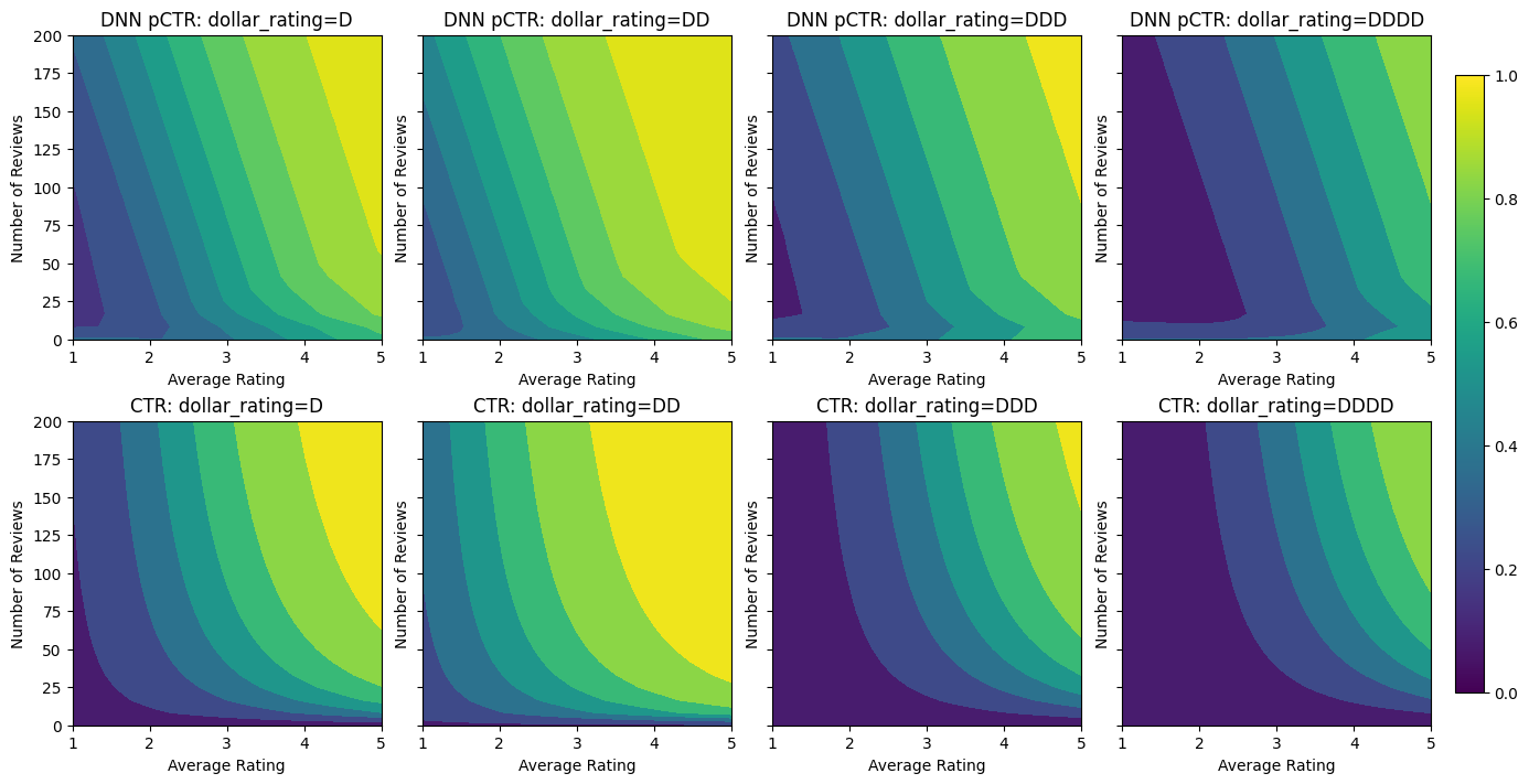
Fitting a DNN
We can repeat the same steps with a DNN classifier. We can observe a similar pattern: not having enough sample points with small number of reviews results in nonsensical extrapolation.
keras.utils.set_random_seed(42)
inputs = {
"num_reviews": keras.Input(shape=(1,), dtype=tf.float32),
"avg_rating": keras.Input(shape=(1), dtype=tf.float32),
"dollar_rating": keras.Input(shape=(1), dtype=tf.string),
}
inputs_flat = keras.layers.Concatenate()([
inputs["num_reviews"],
inputs["avg_rating"],
keras.layers.StringLookup(
vocabulary=dollar_ratings_vocab,
num_oov_indices=0,
output_mode="one_hot",
)(inputs["dollar_rating"]),
])
dense_layers = keras.Sequential(
[
keras.layers.Dense(16, activation="relu"),
keras.layers.Dense(16, activation="relu"),
keras.layers.Dense(1, activation=None),
],
name="dense_layers",
)
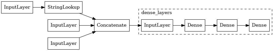
dnn_model = keras.Model(inputs=inputs, outputs=dense_layers(inputs_flat))
keras.utils.plot_model(
dnn_model, expand_nested=True, show_layer_names=False, rankdir="LR"
)
dnn_model.compile(
    loss=keras.losses.BinaryCrossentropy(from_logits=True),
    metrics=[keras.metrics.AUC(from_logits=True, name="auc")],
    optimizer=keras.optimizers.Adam(LEARNING_RATE),
)
dnn_model.fit(ds_train, epochs=200, verbose=0)
analyze_model([(dnn_model, "DNN")], from_logits=True)
Validation AUC: 0.7568147778511047
Testing AUC: 0.8183510899543762
Shape Constraints
TensorFlow Lattice (TFL) is focused on enforcing shape constraints to safeguard model behavior beyond the training data. These shape constraints are applied to TFL Keras layers. Their details can be found in our JMLR paper.
In this tutorial we use TF premade models to cover various shape constraints, but note that all these steps can be done with models created from TFL Keras layers.
Using TFL premade models also requires:
- a model config: defining the model architecture and per-feature shape constraints and regularizers.
- a feature analysis dataset: a dataset used for TFL initialization (feature quantile calcuation).
For a more thorough description, please refer to the premade models or the API docs.
Monotonicity
We first address the monotonicity concerns by adding monotonicity shape constraints to the continuous features. We use a calibrated lattice model with added output calibration: each feature is calibrated using categorical or piecewise-linear calibrators, then fed into a lattice model, followed by an output piecewise-linear calibrator.
To instruct TFL to enforce shape constraints, we specify the constraints in the feature configs. The following code shows how we can require the output to be monotonically increasing with respect to both num_reviews and avg_rating by setting monotonicity="increasing".
model_config = tfl.configs.CalibratedLatticeConfig(
    feature_configs=[
        tfl.configs.FeatureConfig(
            name="num_reviews",
            lattice_size=3,
            monotonicity="increasing",
            pwl_calibration_num_keypoints=32,
        ),
        tfl.configs.FeatureConfig(
            name="avg_rating",
            lattice_size=3,
            monotonicity="increasing",
            pwl_calibration_num_keypoints=32,
        ),
        tfl.configs.FeatureConfig(
            name="dollar_rating",
            lattice_size=3,
            pwl_calibration_num_keypoints=4,
            vocabulary_list=dollar_ratings_vocab,
            num_buckets=len(dollar_ratings_vocab),
        ),
    ],
    output_calibration=True,
    output_initialization=np.linspace(-2, 2, num=5),
)
We now use the feature_analysis_data to find and set the quantile values for the input features. These values can be pre-calculated and set explicitly in the feature config depending on the training pipeline.
feature_analysis_data = data_train.copy()
feature_analysis_data["dollar_rating"] = feature_analysis_data[
    "dollar_rating"
].map({v: i for i, v in enumerate(dollar_ratings_vocab)})
feature_analysis_data = dict(feature_analysis_data)

feature_keypoints = tfl.premade_lib.compute_feature_keypoints(
    feature_configs=model_config.feature_configs, features=feature_analysis_data
)
tfl.premade_lib.set_feature_keypoints(
    feature_configs=model_config.feature_configs,
    feature_keypoints=feature_keypoints,
    add_missing_feature_configs=False,
)
keras.utils.set_random_seed(42)
inputs = {
    "num_reviews": keras.Input(shape=(1,), dtype=tf.float32),
    "avg_rating": keras.Input(shape=(1), dtype=tf.float32),
    "dollar_rating": keras.Input(shape=(1), dtype=tf.string),
}
ordered_inputs = [
    inputs["num_reviews"],
    inputs["avg_rating"],
    keras.layers.StringLookup(
        vocabulary=dollar_ratings_vocab,
        num_oov_indices=0,
        output_mode="int",
    )(inputs["dollar_rating"]),
]
outputs = tfl.premade.CalibratedLattice(
    model_config=model_config, name="CalibratedLattice"
)(ordered_inputs)
tfl_model_0 = keras.Model(inputs=inputs, outputs=outputs)

keras.utils.plot_model(
    tfl_model_0, expand_nested=True, show_layer_names=False, rankdir="LR"
)
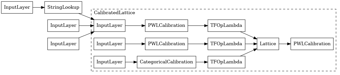
Using a CalibratedLatticeConfig creates a premade classifier that first applies a calibrator to each input (a piece-wise linear function for numeric features) followed by a lattice layer to non-linearly fuse the calibrated features. We have also enabled output piece-wise linear calibration.
tfl_model_0.compile(
    loss=keras.losses.BinaryCrossentropy(from_logits=True),
    metrics=[keras.metrics.AUC(from_logits=True, name="auc")],
    optimizer=keras.optimizers.Adam(LEARNING_RATE),
)
tfl_model_0.fit(ds_train, epochs=100, verbose=0)
analyze_model([(tfl_model_0, "TFL0")], from_logits=True)
Validation AUC: 0.7199402451515198
Testing AUC: 0.798313558101654
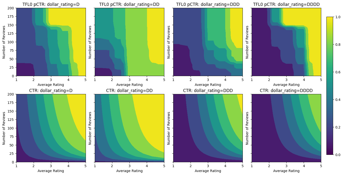
With the constraints added, the estimated CTR will always increase as the average rating increases or the number of reviews increases. This is done by making sure that the calibrators and the lattice are monotonic.
Partial Monotonicity for Categorical Calibration
To use constraints on the third feature, dollar_rating, we should recall that categorical features require a slightly different treatment in TFL. Here we enforce the partial monotonicity constraint that outputs for "DD" restaurants should be larger than "D" restaurants when all other inputs are fixed. This is done using the monotonicity setting in the feature config. We also need to use tfl.premade_lib.set_categorical_monotonicities to convert the constrains specified in string values into the numerical format understood by the library.
keras.utils.set_random_seed(42)
model_config = tfl.configs.CalibratedLatticeConfig(
    feature_configs=[
        tfl.configs.FeatureConfig(
            name="num_reviews",
            lattice_size=3,
            monotonicity="increasing",
            pwl_calibration_convexity="concave",
            pwl_calibration_num_keypoints=32,
        ),
        tfl.configs.FeatureConfig(
            name="avg_rating",
            lattice_size=3,
            monotonicity="increasing",
            pwl_calibration_num_keypoints=32,
        ),
        tfl.configs.FeatureConfig(
            name="dollar_rating",
            lattice_size=3,
            pwl_calibration_num_keypoints=4,
            vocabulary_list=dollar_ratings_vocab,
            num_buckets=len(dollar_ratings_vocab),
            monotonicity=[("D", "DD")],
        ),
    ],
    output_calibration=True,
    output_initialization=np.linspace(-2, 2, num=5),
)

tfl.premade_lib.set_feature_keypoints(
    feature_configs=model_config.feature_configs,
    feature_keypoints=feature_keypoints,
    add_missing_feature_configs=False,
)
tfl.premade_lib.set_categorical_monotonicities(model_config.feature_configs)

outputs = tfl.premade.CalibratedLattice(
    model_config=model_config, name="CalibratedLattice"
)(ordered_inputs)
tfl_model_1 = keras.Model(inputs=inputs, outputs=outputs)
tfl_model_1.compile(
    loss=keras.losses.BinaryCrossentropy(from_logits=True),
    metrics=[keras.metrics.AUC(from_logits=True, name="auc")],
    optimizer=keras.optimizers.Adam(LEARNING_RATE),
)
tfl_model_1.fit(ds_train, epochs=100, verbose=0)
analyze_model([(tfl_model_1, "TFL1")], from_logits=True)
Validation AUC: 0.741411566734314
Testing AUC: 0.8500608205795288
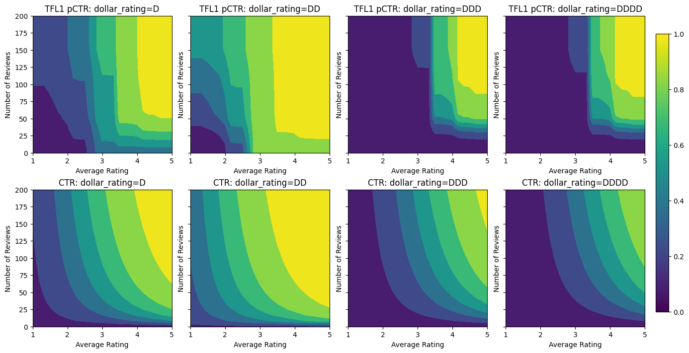
Here we also plot the predicted CTR of this model conditioned on dollar_rating. Notice that all the constraints we required are fulfilled in each of the slices.
2D Shape Constraint: Trust
A 5-star rating for a restaurant with only one or two reviews is likely an unreliable rating (the restaurant might not actually be good), whereas a 4-star rating for a restaurant with hundreds of reviews is much more reliable (the restaurant is likely good in this case). We can see that the number of reviews of a restaurant affects how much trust we place in its average rating.
We can exercise TFL trust constraints to inform the model that the larger (or smaller) value of one feature indicates more reliance or trust of another feature. This is done by setting reflects_trust_in configuration in the feature config.
keras.utils.set_random_seed(42)
model_config = tfl.configs.CalibratedLatticeConfig(
    feature_configs=[
        tfl.configs.FeatureConfig(
            name="num_reviews",
            lattice_size=3,
            monotonicity="increasing",
            pwl_calibration_num_keypoints=32,
            # Larger num_reviews indicating more trust in avg_rating.
            reflects_trust_in=[
                tfl.configs.TrustConfig(
                    feature_name="avg_rating", trust_type="edgeworth"
                ),
            ],
        ),
        tfl.configs.FeatureConfig(
            name="avg_rating",
            lattice_size=3,
            monotonicity="increasing",
            pwl_calibration_num_keypoints=32,
        ),
        tfl.configs.FeatureConfig(
            name="dollar_rating",
            lattice_size=3,
            pwl_calibration_num_keypoints=4,
            vocabulary_list=dollar_ratings_vocab,
            num_buckets=len(dollar_ratings_vocab),
            monotonicity=[("D", "DD")],
        ),
    ],
    output_calibration=True,
    output_initialization=np.linspace(-2, 2, num=5),
)

tfl.premade_lib.set_feature_keypoints(
    feature_configs=model_config.feature_configs,
    feature_keypoints=feature_keypoints,
    add_missing_feature_configs=False,
)
tfl.premade_lib.set_categorical_monotonicities(model_config.feature_configs)

outputs = tfl.premade.CalibratedLattice(
    model_config=model_config, name="CalibratedLattice"
)(ordered_inputs)
tfl_model_2 = keras.Model(inputs=inputs, outputs=outputs)
tfl_model_2.compile(
    loss=keras.losses.BinaryCrossentropy(from_logits=True),
    metrics=[keras.metrics.AUC(from_logits=True, name="auc")],
    optimizer=keras.optimizers.Adam(LEARNING_RATE),
)
tfl_model_2.fit(ds_train, epochs=100, verbose=0)
analyze_model([(tfl_model_2, "TFL2")], from_logits=True)
Validation AUC: 0.774645209312439
Testing AUC: 0.8462862372398376
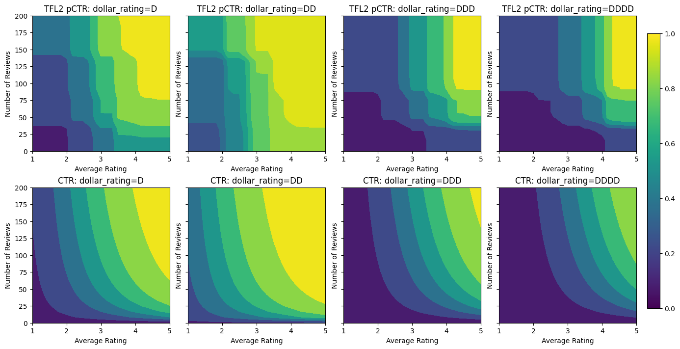
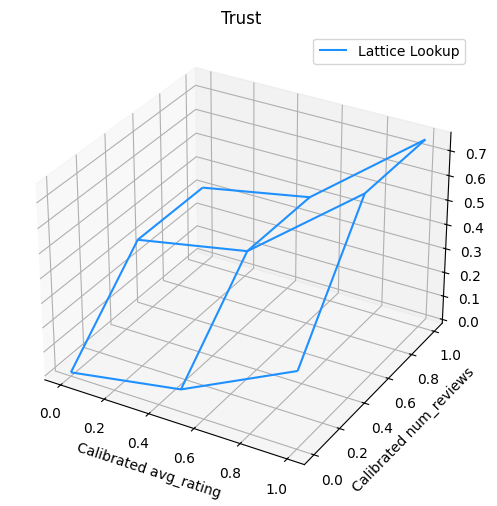
The following plot presents the trained lattice function. Due to the trust constraint, we expect that larger values of calibrated num_reviews would force higher slope with respect to calibrated avg_rating, resulting in a more significant move in the lattice output.
lattice_params = tfl_model_2.layers[-1].layers[-2].weights[0].numpy()
lat_mesh_x, lat_mesh_y = np.meshgrid(
    np.linspace(0, 1, num=3),
    np.linspace(0, 1, num=3),
)
lat_mesh_z = np.reshape(np.asarray(lattice_params[0::3]), (3, 3))

figure = plt.figure(figsize=(6, 6))
axes = figure.add_subplot(projection="3d")
axes.plot_wireframe(lat_mesh_x, lat_mesh_y, lat_mesh_z, color="dodgerblue")
plt.legend(["Lattice Lookup"])
plt.title("Trust")
plt.xlabel("Calibrated avg_rating")
plt.ylabel("Calibrated num_reviews")
plt.show()
Diminishing Returns
Diminishing returns means that the marginal gain of increasing a certain feature value will decrease as we increase the value. In our case we expect that the num_reviews feature follows this pattern, so we can configure its calibrator accordingly. Notice that we can decompose diminishing returns into two sufficient conditions:
- the calibrator is monotonicially increasing, and
- the calibrator is concave (setting
pwl_calibration_convexity="concave").
keras.utils.set_random_seed(42)
model_config = tfl.configs.CalibratedLatticeConfig(
    feature_configs=[
        tfl.configs.FeatureConfig(
            name="num_reviews",
            lattice_size=3,
            monotonicity="increasing",
            pwl_calibration_convexity="concave",
            pwl_calibration_num_keypoints=32,
            reflects_trust_in=[
                tfl.configs.TrustConfig(
                    feature_name="avg_rating", trust_type="edgeworth"
                ),
            ],
        ),
        tfl.configs.FeatureConfig(
            name="avg_rating",
            lattice_size=3,
            monotonicity="increasing",
            pwl_calibration_num_keypoints=32,
        ),
        tfl.configs.FeatureConfig(
            name="dollar_rating",
            lattice_size=3,
            pwl_calibration_num_keypoints=4,
            vocabulary_list=dollar_ratings_vocab,
            num_buckets=len(dollar_ratings_vocab),
            monotonicity=[("D", "DD")],
        ),
    ],
    output_calibration=True,
    output_initialization=np.linspace(-2, 2, num=5),
)

tfl.premade_lib.set_feature_keypoints(
    feature_configs=model_config.feature_configs,
    feature_keypoints=feature_keypoints,
    add_missing_feature_configs=False,
)
tfl.premade_lib.set_categorical_monotonicities(model_config.feature_configs)

outputs = tfl.premade.CalibratedLattice(
    model_config=model_config, name="CalibratedLattice"
)(ordered_inputs)
tfl_model_3 = keras.Model(inputs=inputs, outputs=outputs)
tfl_model_3.compile(
    loss=keras.losses.BinaryCrossentropy(from_logits=True),
    metrics=[keras.metrics.AUC(from_logits=True, name="auc")],
    optimizer=keras.optimizers.Adam(LEARNING_RATE),
)
tfl_model_3.fit(
    ds_train,
    epochs=100,
    verbose=0
)
analyze_model([(tfl_model_3, "TFL3")], from_logits=True)
Validation AUC: 0.7506535053253174
Testing AUC: 0.8575603365898132
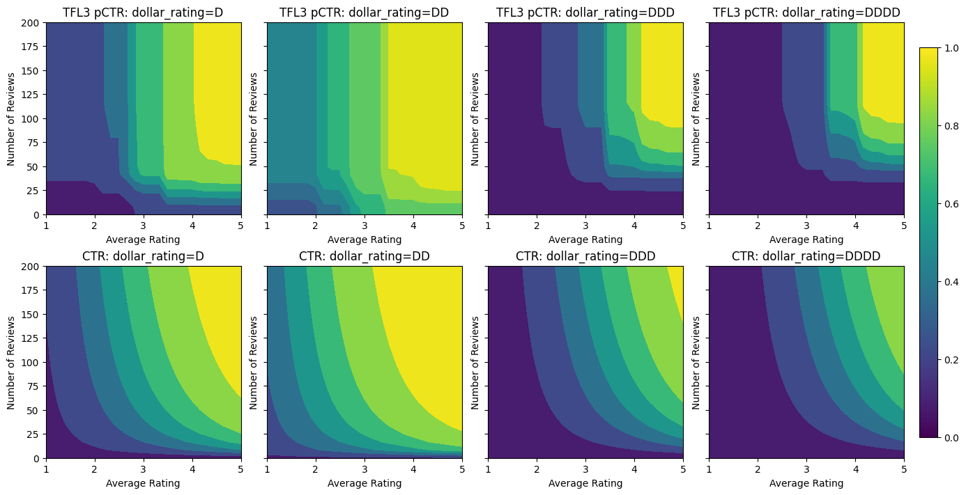
Notice how the testing metric improves by adding the concavity constraint. The prediction plot also better resembles the ground truth.
Smoothing Calibrators
We notice in the prediction curves above that even though the output is monotonic in specified features, the changes in the slopes are abrupt and hard to interpret. That suggests we might want to consider smoothing this calibrator using a regularizer setup in the regularizer_configs.
Here we apply a hessian regularizer to make the calibration more linear. You can also use the laplacian regularizer to flatten the calibrator and the wrinkle regularizer to reduce changes in the curvature.
keras.utils.set_random_seed(42)
model_config = tfl.configs.CalibratedLatticeConfig(
    feature_configs=[
        tfl.configs.FeatureConfig(
            name="num_reviews",
            lattice_size=3,
            monotonicity="increasing",
            pwl_calibration_convexity="concave",
            pwl_calibration_num_keypoints=32,
            regularizer_configs=[
                tfl.configs.RegularizerConfig(name="calib_hessian", l2=0.5),
            ],
            reflects_trust_in=[
                tfl.configs.TrustConfig(
                    feature_name="avg_rating", trust_type="edgeworth"
                ),
            ],
        ),
        tfl.configs.FeatureConfig(
            name="avg_rating",
            lattice_size=3,
            monotonicity="increasing",
            pwl_calibration_num_keypoints=32,
            regularizer_configs=[
                tfl.configs.RegularizerConfig(name="calib_hessian", l2=0.5),
            ],
        ),
        tfl.configs.FeatureConfig(
            name="dollar_rating",
            lattice_size=3,
            pwl_calibration_num_keypoints=4,
            vocabulary_list=dollar_ratings_vocab,
            num_buckets=len(dollar_ratings_vocab),
            monotonicity=[("D", "DD")],
        ),
    ],
    output_calibration=True,
    output_initialization=np.linspace(-2, 2, num=5),
    regularizer_configs=[
        tfl.configs.RegularizerConfig(name="calib_hessian", l2=0.1),
    ],
)

tfl.premade_lib.set_feature_keypoints(
    feature_configs=model_config.feature_configs,
    feature_keypoints=feature_keypoints,
    add_missing_feature_configs=False,
)
tfl.premade_lib.set_categorical_monotonicities(model_config.feature_configs)

outputs = tfl.premade.CalibratedLattice(
    model_config=model_config, name="CalibratedLattice"
)(ordered_inputs)
tfl_model_4 = keras.Model(inputs=inputs, outputs=outputs)
tfl_model_4.compile(
    loss=keras.losses.BinaryCrossentropy(from_logits=True),
    metrics=[keras.metrics.AUC(from_logits=True, name="auc")],
    optimizer=keras.optimizers.Adam(LEARNING_RATE),
)
tfl_model_4.fit(ds_train, epochs=100, verbose=0)
analyze_model([(tfl_model_4, "TFL4")], from_logits=True)
Validation AUC: 0.7562546730041504
Testing AUC: 0.8593733310699463
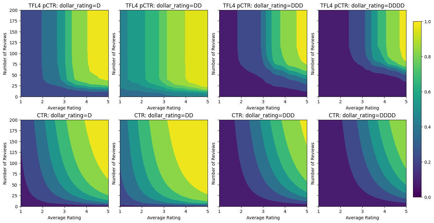
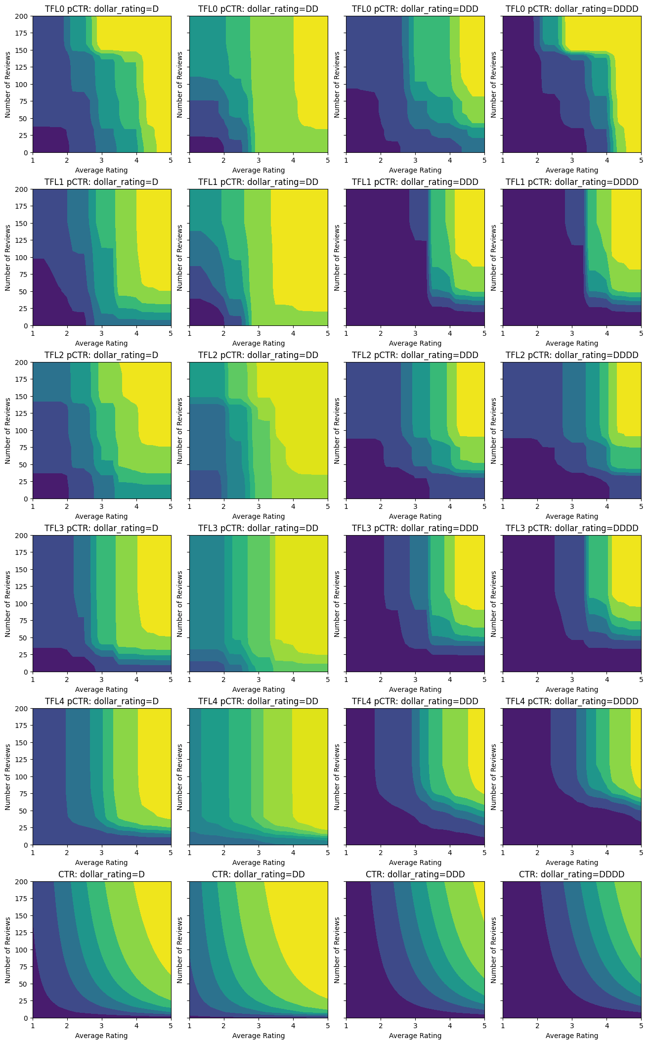
The calibrators are now smooth, and the overall estimated CTR better matches the ground truth. This is reflected both in the testing metric and in the contour plots.
Here you can see the results of each step as we added domain-specific constraints and regularizers to the model.
analyze_model(
    [
        (tfl_model_0, "TFL0"),
        (tfl_model_1, "TFL1"),
        (tfl_model_2, "TFL2"),
        (tfl_model_3, "TFL3"),
        (tfl_model_4, "TFL4"),
    ],
    from_logits=True,
    print_metrics=False,
)