|
|
|
 View source on GitHub View source on GitHub
|
|
Overview
This tutorial demonstrates how the TensorFlow Lattice (TFL) library can be used to train models that behave responsibly, and do not violate certain assumptions that are ethical or fair. In particular, we will focus on using monotonicity constraints to avoid unfair penalization of certain attributes. This tutorial includes demonstrations of the experiments from the paper Deontological Ethics By Monotonicity Shape Constraints by Serena Wang and Maya Gupta, published at AISTATS 2020.
We will use TFL premade models on public datasets, but note that everything in this tutorial can also be done with models constructed from TFL Keras layers.
Before proceeding, make sure your runtime has all required packages installed (as imported in the code cells below).
Setup
Installing TF Lattice package:
pip install -U tensorflow tf-keras tensorflow-lattice seaborn pydot graphvizpip install -U tensorflow_decision_forests
Importing required packages:
import tensorflow as tf
import tensorflow_lattice as tfl
import tensorflow_decision_forests as tfdf

import logging
import matplotlib.pyplot as plt
import numpy as np
import os
import pandas as pd
import seaborn as sns
from sklearn.model_selection import train_test_split
import sys
import tempfile
logging.disable(sys.maxsize)
2026-03-06 12:26:01.557159: E external/local_xla/xla/stream_executor/cuda/cuda_fft.cc:467] Unable to register cuFFT factory: Attempting to register factory for plugin cuFFT when one has already been registered
WARNING: All log messages before absl::InitializeLog() is called are written to STDERR
E0000 00:00:1772799961.580269   51492 cuda_dnn.cc:8579] Unable to register cuDNN factory: Attempting to register factory for plugin cuDNN when one has already been registered
E0000 00:00:1772799961.587709   51492 cuda_blas.cc:1407] Unable to register cuBLAS factory: Attempting to register factory for plugin cuBLAS when one has already been registered
W0000 00:00:1772799961.606066   51492 computation_placer.cc:177] computation placer already registered. Please check linkage and avoid linking the same target more than once.
W0000 00:00:1772799961.606086   51492 computation_placer.cc:177] computation placer already registered. Please check linkage and avoid linking the same target more than once.
W0000 00:00:1772799961.606088   51492 computation_placer.cc:177] computation placer already registered. Please check linkage and avoid linking the same target more than once.
W0000 00:00:1772799961.606091   51492 computation_placer.cc:177] computation placer already registered. Please check linkage and avoid linking the same target more than once.
# Use Keras 2.
version_fn = getattr(tf.keras, "version", None)
if version_fn and version_fn().startswith("3."):
  import tf_keras as keras
else:
  keras = tf.keras
Default values used in this tutorial:
# Default number of training epochs, batch sizes and learning rate.
NUM_EPOCHS = 256
BATCH_SIZE = 256
LEARNING_RATES = 0.01
# Directory containing dataset files.
DATA_DIR = 'https://raw.githubusercontent.com/serenalwang/shape_constraints_for_ethics/master'
Case study #1: Law school admissions
In the first part of this tutorial, we will consider a case study using the Law School Admissions dataset from the Law School Admissions Council (LSAC). We will train a classifier to predict whether or not a student will pass the bar using two features: the student's LSAT score and undergraduate GPA.
Suppose that the classifier’s score was used to guide law school admissions or scholarships. According to merit-based social norms, we would expect that students with higher GPA and higher LSAT score should receive a higher score from the classifier. However, we will observe that it is easy for models to violate these intuitive norms, and sometimes penalize people for having a higher GPA or LSAT score.
To address this unfair penalization problem, we can impose monotonicity constraints so that a model never penalizes higher GPA or higher LSAT score, all else equal. In this tutorial, we will show how to impose those monotonicity constraints using TFL.
Load Law School Data
# Load data file.
law_file_name = 'lsac.csv'
law_file_path = os.path.join(DATA_DIR, law_file_name)
raw_law_df = pd.read_csv(law_file_path, delimiter=',')
Preprocess dataset:
# Define label column name.
LAW_LABEL = 'pass_bar'
def preprocess_law_data(input_df):
  # Drop rows with where the label or features of interest are missing.
  output_df = input_df[~input_df[LAW_LABEL].isna() & ~input_df['ugpa'].isna() &
                       (input_df['ugpa'] > 0) & ~input_df['lsat'].isna()]
  return output_df


law_df = preprocess_law_data(raw_law_df)
Split data into train/validation/test sets
def split_dataset(input_df, random_state=888):
  """Splits an input dataset into train, val, and test sets."""
  train_df, test_val_df = train_test_split(
      input_df, test_size=0.3, random_state=random_state
  )
  val_df, test_df = train_test_split(
      test_val_df, test_size=0.66, random_state=random_state
  )
  return train_df, val_df, test_df


dataframes = {}
datasets = {}

(dataframes['law_train'], dataframes['law_val'], dataframes['law_test']) = (
    split_dataset(law_df)
)

for df_name, df in dataframes.items():
  datasets[df_name] = tf.data.Dataset.from_tensor_slices(
      ((df[['ugpa']], df[['lsat']]), df[['pass_bar']])
  ).batch(BATCH_SIZE)
2026-03-06 12:26:05.388088: E external/local_xla/xla/stream_executor/cuda/cuda_platform.cc:51] failed call to cuInit: INTERNAL: CUDA error: Failed call to cuInit: CUDA_ERROR_NO_DEVICE: no CUDA-capable device is detected
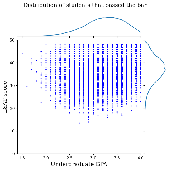
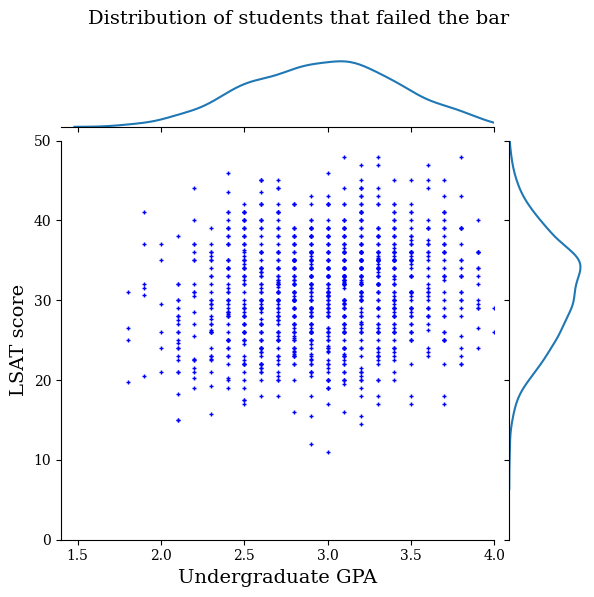
Visualize data distribution
First we will visualize the distribution of the data. We will plot the GPA and LSAT scores for all students that passed the bar and also for all students that did not pass the bar.
def plot_dataset_contour(input_df, title):
  plt.rcParams['font.family'] = ['serif']
  g = sns.jointplot(
      x='ugpa',
      y='lsat',
      data=input_df,
      kind='kde',
      xlim=[1.4, 4],
      ylim=[0, 50])
  g.plot_joint(plt.scatter, c='b', s=10, linewidth=1, marker='+')
  g.ax_joint.collections[0].set_alpha(0)
  g.set_axis_labels('Undergraduate GPA', 'LSAT score', fontsize=14)
  g.fig.suptitle(title, fontsize=14)
  # Adust plot so that the title fits.
  plt.subplots_adjust(top=0.9)
  plt.show()
law_df_pos = law_df[law_df[LAW_LABEL] == 1]
plot_dataset_contour(
    law_df_pos, title='Distribution of students that passed the bar')
law_df_neg = law_df[law_df[LAW_LABEL] == 0]
plot_dataset_contour(
    law_df_neg, title='Distribution of students that failed the bar')
Train calibrated lattice model to predict bar exam passage
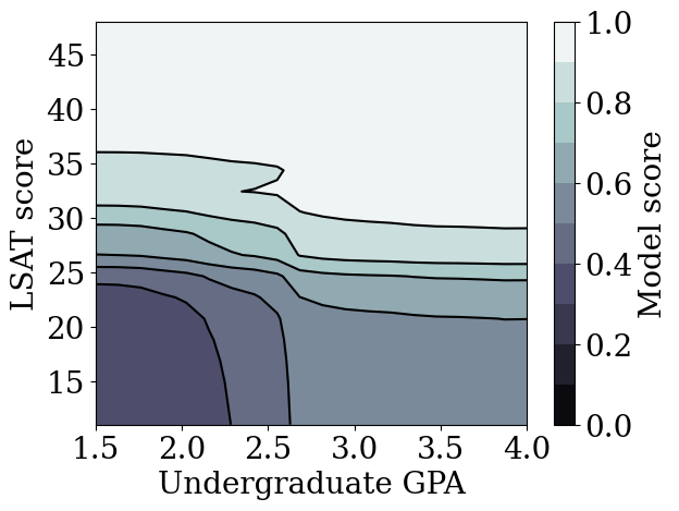
Next, we will train a calibrated lattice model from TFL to predict whether or not a student will pass the bar. The two input features will be LSAT score and undergraduate GPA, and the training label will be whether the student passed the bar.
We will first train a calibrated lattice model without any constraints. Then, we will train a calibrated lattice model with monotonicity constraints and observe the difference in the model output and accuracy.
Helper functions for visualization of trained model outputs
def plot_model_contour(model, from_logits=False, num_keypoints=20):
  x = np.linspace(min(law_df['ugpa']), max(law_df['ugpa']), num_keypoints)
  y = np.linspace(min(law_df['lsat']), max(law_df['lsat']), num_keypoints)

  x_grid, y_grid = np.meshgrid(x, y)

  positions = np.vstack([x_grid.ravel(), y_grid.ravel()])
  plot_df = pd.DataFrame(positions.T, columns=['ugpa', 'lsat'])
  plot_df[LAW_LABEL] = np.ones(len(plot_df))
  predictions = model.predict((plot_df[['ugpa']], plot_df[['lsat']]))
  if from_logits:
    predictions = tf.math.sigmoid(predictions)
  grid_predictions = np.reshape(predictions, x_grid.shape)

  plt.rcParams['font.family'] = ['serif']
  plt.contour(
      x_grid,
      y_grid,
      grid_predictions,
      colors=('k',),
      levels=np.linspace(0, 1, 11),
  )
  plt.contourf(
      x_grid,
      y_grid,
      grid_predictions,
      cmap=plt.cm.bone,
      levels=np.linspace(0, 1, 11),
  )
  plt.xticks(fontsize=20)
  plt.yticks(fontsize=20)

  cbar = plt.colorbar()
  cbar.ax.set_ylabel('Model score', fontsize=20)
  cbar.ax.tick_params(labelsize=20)

  plt.xlabel('Undergraduate GPA', fontsize=20)
  plt.ylabel('LSAT score', fontsize=20)
Train unconstrained (non-monotonic) calibrated lattice model
We create a TFL premade model using a 'CalibratedLatticeConfig. This model is a calibrated lattice model with an output calibration.
model_config = tfl.configs.CalibratedLatticeConfig(
    feature_configs=[
        tfl.configs.FeatureConfig(
            name='ugpa',
            lattice_size=3,
            pwl_calibration_num_keypoints=16,
            monotonicity=0,
            pwl_calibration_always_monotonic=False,
        ),
        tfl.configs.FeatureConfig(
            name='lsat',
            lattice_size=3,
            pwl_calibration_num_keypoints=16,
            monotonicity=0,
            pwl_calibration_always_monotonic=False,
        ),
    ],
    output_calibration=True,
    output_initialization=np.linspace(-2, 2, num=8),
)
We calculate and populate feature quantiles in the feature configs using the premade_lib API.
feature_keypoints = tfl.premade_lib.compute_feature_keypoints(
    feature_configs=model_config.feature_configs,
    features=dataframes['law_train'][['ugpa', 'lsat', 'pass_bar']],
)
tfl.premade_lib.set_feature_keypoints(
    feature_configs=model_config.feature_configs,
    feature_keypoints=feature_keypoints,
    add_missing_feature_configs=False,
)
nomon_lattice_model = tfl.premade.CalibratedLattice(model_config=model_config)
keras.utils.plot_model(
    nomon_lattice_model, expand_nested=True, show_layer_names=False, rankdir="LR"
)

nomon_lattice_model.compile(
    loss=keras.losses.BinaryCrossentropy(from_logits=True),
    metrics=[
        keras.metrics.BinaryAccuracy(name='accuracy'),
    ],
    optimizer=keras.optimizers.Adam(LEARNING_RATES),
)
nomon_lattice_model.fit(datasets['law_train'], epochs=NUM_EPOCHS, verbose=0)

train_acc = nomon_lattice_model.evaluate(datasets['law_train'])[1]
val_acc = nomon_lattice_model.evaluate(datasets['law_val'])[1]
test_acc = nomon_lattice_model.evaluate(datasets['law_test'])[1]
print(
    'accuracies for train: %f, val: %f, test: %f'
    % (train_acc, val_acc, test_acc)
)
63/63 [==============================] - 0s 1ms/step - loss: 0.1727 - accuracy: 0.9460
10/10 [==============================] - 0s 1ms/step - loss: 0.1877 - accuracy: 0.9390
18/18 [==============================] - 0s 1ms/step - loss: 0.1672 - accuracy: 0.9480
accuracies for train: 0.945995, val: 0.939003, test: 0.948020
plot_model_contour(nomon_lattice_model, from_logits=True)
13/13 [==============================] - 0s 1ms/step
Train monotonic calibrated lattice model
We can get a monotonic model by setting the monotonicity constraints in feature configs.
model_config.feature_configs[0].monotonicity = 1
model_config.feature_configs[1].monotonicity = 1
mon_lattice_model = tfl.premade.CalibratedLattice(model_config=model_config)

mon_lattice_model.compile(
    loss=keras.losses.BinaryCrossentropy(from_logits=True),
    metrics=[
        keras.metrics.BinaryAccuracy(name='accuracy'),
    ],
    optimizer=keras.optimizers.Adam(LEARNING_RATES),
)
mon_lattice_model.fit(datasets['law_train'], epochs=NUM_EPOCHS, verbose=0)

train_acc = mon_lattice_model.evaluate(datasets['law_train'])[1]
val_acc = mon_lattice_model.evaluate(datasets['law_val'])[1]
test_acc = mon_lattice_model.evaluate(datasets['law_test'])[1]
print(
    'accuracies for train: %f, val: %f, test: %f'
    % (train_acc, val_acc, test_acc)
)
63/63 [==============================] - 0s 1ms/step - loss: 0.1712 - accuracy: 0.9463
10/10 [==============================] - 0s 2ms/step - loss: 0.1869 - accuracy: 0.9403
18/18 [==============================] - 0s 2ms/step - loss: 0.1654 - accuracy: 0.9487
accuracies for train: 0.946308, val: 0.940292, test: 0.948684
plot_model_contour(mon_lattice_model, from_logits=True)
13/13 [==============================] - 0s 1ms/step
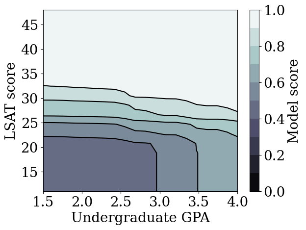
We demonstrated that TFL calibrated lattice models could be trained to be monotonic in both LSAT score and GPA without too big of a sacrifice in accuracy.
Train other unconstrained models
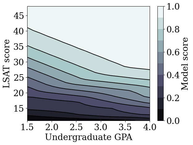
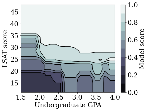
How does the calibrated lattice model compare to other types of models, like deep neural networks (DNNs) or gradient boosted trees (GBTs)? Do DNNs and GBTs appear to have reasonably fair outputs? To address this question, we will next train an unconstrained DNN and GBT. In fact, we will observe that the DNN and GBT both easily violate monotonicity in LSAT score and undergraduate GPA.
Train an unconstrained Deep Neural Network (DNN) model
The architecture was previously optimized to achieve high validation accuracy.
keras.utils.set_random_seed(42)
inputs = [
    keras.Input(shape=(1,), dtype=tf.float32),
    keras.Input(shape=(1), dtype=tf.float32),
]
inputs_flat = keras.layers.Concatenate()(inputs)
dense_layers = keras.Sequential(
    [
        keras.layers.Dense(64, activation='relu'),
        keras.layers.Dense(32, activation='relu'),
        keras.layers.Dense(1, activation=None),
    ],
    name='dense_layers',
)
dnn_model = keras.Model(inputs=inputs, outputs=dense_layers(inputs_flat))
dnn_model.compile(
    loss=keras.losses.BinaryCrossentropy(from_logits=True),
    metrics=[keras.metrics.BinaryAccuracy(name='accuracy')],
    optimizer=keras.optimizers.Adam(LEARNING_RATES),
)
dnn_model.fit(datasets['law_train'], epochs=NUM_EPOCHS, verbose=0)

train_acc = dnn_model.evaluate(datasets['law_train'])[1]
val_acc = dnn_model.evaluate(datasets['law_val'])[1]
test_acc = dnn_model.evaluate(datasets['law_test'])[1]
print(
    'accuracies for train: %f, val: %f, test: %f'
    % (train_acc, val_acc, test_acc)
)
63/63 [==============================] - 0s 1ms/step - loss: 0.1729 - accuracy: 0.9482
10/10 [==============================] - 0s 1ms/step - loss: 0.1846 - accuracy: 0.9424
18/18 [==============================] - 0s 1ms/step - loss: 0.1658 - accuracy: 0.9505
accuracies for train: 0.948248, val: 0.942440, test: 0.950453
plot_model_contour(dnn_model, from_logits=True)
13/13 [==============================] - 0s 1ms/step
Train an unconstrained Gradient Boosted Trees (GBT) model
The tree structure was previously optimized to achieve high validation accuracy.
tree_model = tfdf.keras.GradientBoostedTreesModel(
    exclude_non_specified_features=False,
    num_threads=1,
    num_trees=20,
    max_depth=4,
    growing_strategy='BEST_FIRST_GLOBAL',
    random_seed=42,
    temp_directory=tempfile.mkdtemp(),
)
tree_model.compile(metrics=[keras.metrics.BinaryAccuracy(name='accuracy')])
tree_model.fit(
    datasets['law_train'], validation_data=datasets['law_val'], verbose=0
)

tree_train_acc = tree_model.evaluate(datasets['law_train'], verbose=0)[1]
tree_val_acc = tree_model.evaluate(datasets['law_val'], verbose=0)[1]
tree_test_acc = tree_model.evaluate(datasets['law_test'], verbose=0)[1]
print(
    'accuracies for GBT: train: %f, val: %f, test: %f'
    % (tree_train_acc, tree_val_acc, tree_test_acc)
)
WARNING: All log messages before absl::InitializeLog() is called are written to STDERR
W0000 00:00:1772800062.439122   51492 gradient_boosted_trees.cc:1873] "goss_alpha" set but "sampling_method" not equal to "GOSS".
W0000 00:00:1772800062.439186   51492 gradient_boosted_trees.cc:1883] "goss_beta" set but "sampling_method" not equal to "GOSS".
W0000 00:00:1772800062.439190   51492 gradient_boosted_trees.cc:1897] "selective_gradient_boosting_ratio" set but "sampling_method" not equal to "SELGB".
Num validation examples: tf.Tensor(2328, shape=(), dtype=int32)
I0000 00:00:1772800066.147549   51492 kernel.cc:782] Start Yggdrasil model training
I0000 00:00:1772800066.147584   51492 kernel.cc:783] Collect training examples
I0000 00:00:1772800066.147593   51492 kernel.cc:795] Dataspec guide:
column_guides {
  column_name_pattern: "^__LABEL$"
  type: CATEGORICAL
  categorial {
    min_vocab_frequency: 0
    max_vocab_count: -1
  }
}
default_column_guide {
  categorial {
    max_vocab_count: 2000
  }
  discretized_numerical {
    maximum_num_bins: 255
  }
}
ignore_columns_without_guides: false
detect_numerical_as_discretized_numerical: false

I0000 00:00:1772800066.147962   51492 kernel.cc:401] Number of batches: 63
I0000 00:00:1772800066.147977   51492 kernel.cc:402] Number of examples: 15980
I0000 00:00:1772800066.148312   51492 kernel.cc:802] Training dataset:
Number of records: 15980
Number of columns: 3

Number of columns by type:
    NUMERICAL: 2 (66.6667%)
    CATEGORICAL: 1 (33.3333%)

Columns:

NUMERICAL: 2 (66.6667%)
    0: "0" NUMERICAL mean:3.22705 min:1.6 max:4 sd:0.415473
    1: "1" NUMERICAL mean:36.8057 min:11 max:48 sd:5.46358

CATEGORICAL: 1 (33.3333%)
    2: "__LABEL" CATEGORICAL integerized vocab-size:3 no-ood-item

Terminology:
    nas: Number of non-available (i.e. missing) values.
    ood: Out of dictionary.
    manually-defined: Attribute whose type is manually defined by the user, i.e., the type was not automatically inferred.
    tokenized: The attribute value is obtained through tokenization.
    has-dict: The attribute is attached to a string dictionary e.g. a categorical attribute stored as a string.
    vocab-size: Number of unique values.

I0000 00:00:1772800066.148334   51492 kernel.cc:807] Collect validation dataset
I0000 00:00:1772800066.148348   51492 kernel.cc:401] Number of batches: 10
I0000 00:00:1772800066.148351   51492 kernel.cc:402] Number of examples: 2328
I0000 00:00:1772800066.148401   51492 kernel.cc:813] Validation dataset:
Number of records: 2328
Number of columns: 3

Number of columns by type:
    NUMERICAL: 2 (66.6667%)
    CATEGORICAL: 1 (33.3333%)

Columns:

NUMERICAL: 2 (66.6667%)
    0: "0" NUMERICAL mean:3.23239 min:1.8 max:4 sd:0.403059
    1: "1" NUMERICAL mean:36.8697 min:17 max:48 sd:5.51876

CATEGORICAL: 1 (33.3333%)
    2: "__LABEL" CATEGORICAL integerized vocab-size:3 no-ood-item

Terminology:
    nas: Number of non-available (i.e. missing) values.
    ood: Out of dictionary.
    manually-defined: Attribute whose type is manually defined by the user, i.e., the type was not automatically inferred.
    tokenized: The attribute value is obtained through tokenization.
    has-dict: The attribute is attached to a string dictionary e.g. a categorical attribute stored as a string.
    vocab-size: Number of unique values.

I0000 00:00:1772800066.148412   51492 kernel.cc:818] Configure learner
W0000 00:00:1772800066.148610   51492 gradient_boosted_trees.cc:1873] "goss_alpha" set but "sampling_method" not equal to "GOSS".
W0000 00:00:1772800066.148619   51492 gradient_boosted_trees.cc:1883] "goss_beta" set but "sampling_method" not equal to "GOSS".
W0000 00:00:1772800066.148622   51492 gradient_boosted_trees.cc:1897] "selective_gradient_boosting_ratio" set but "sampling_method" not equal to "SELGB".
I0000 00:00:1772800066.148660   51492 kernel.cc:831] Training config:
learner: "GRADIENT_BOOSTED_TREES"
features: "^0$"
features: "^1$"
label: "^__LABEL$"
task: CLASSIFICATION
random_seed: 42
metadata {
  framework: "TF Keras"
}
pure_serving_model: false
[yggdrasil_decision_forests.model.gradient_boosted_trees.proto.gradient_boosted_trees_config] {
  num_trees: 20
  decision_tree {
    max_depth: 4
    min_examples: 5
    in_split_min_examples_check: true
    keep_non_leaf_label_distribution: true
    num_candidate_attributes: -1
    missing_value_policy: GLOBAL_IMPUTATION
    allow_na_conditions: false
    categorical_set_greedy_forward {
      sampling: 0.1
      max_num_items: -1
      min_item_frequency: 1
    }
    growing_strategy_best_first_global {
    }
    categorical {
      cart {
      }
    }
    axis_aligned_split {
    }
    internal {
      sorting_strategy: PRESORTED
    }
    uplift {
      min_examples_in_treatment: 5
      split_score: KULLBACK_LEIBLER
    }
    numerical_vector_sequence {
      max_num_test_examples: 1000
      num_random_selected_anchors: 100
    }
  }
  shrinkage: 0.1
  loss: DEFAULT
  validation_set_ratio: 0.1
  validation_interval_in_trees: 1
  early_stopping: VALIDATION_LOSS_INCREASE
  early_stopping_num_trees_look_ahead: 30
  l2_regularization: 0
  lambda_loss: 1
  mart {
  }
  adapt_subsample_for_maximum_training_duration: false
  l1_regularization: 0
  use_hessian_gain: false
  l2_regularization_categorical: 1
  xe_ndcg {
    ndcg_truncation: 5
  }
  stochastic_gradient_boosting {
    ratio: 1
  }
  apply_link_function: true
  compute_permutation_variable_importance: false
  early_stopping_initial_iteration: 10
}

I0000 00:00:1772800066.148958   51492 kernel.cc:834] Deployment config:
cache_path: "/tmpfs/tmp/tmpprw0xmor/working_cache"
num_threads: 1
try_resume_training: true

I0000 00:00:1772800066.149150   78713 kernel.cc:895] Train model
I0000 00:00:1772800066.149265   78713 gradient_boosted_trees.cc:577] Default loss set to BINOMIAL_LOG_LIKELIHOOD
I0000 00:00:1772800066.149298   78713 gradient_boosted_trees.cc:1190] Training gradient boosted tree on 15980 example(s) and 2 feature(s).
I0000 00:00:1772800066.149322   78713 gradient_boosted_trees.cc:1230] 15980 examples used for training and 2328 examples used for validation
I0000 00:00:1772800066.152779   78713 gpu.cc:93] Cannot initialize GPU: Not compiled with GPU support
I0000 00:00:1772800066.156703   78713 gradient_boosted_trees.cc:1632] Train tree 1/20 train-loss:0.385271 train-accuracy:0.948436 valid-loss:0.404175 valid-accuracy:0.946306 [total:0.00s iter:0.00s]
I0000 00:00:1772800066.160176   78713 gradient_boosted_trees.cc:1632] Train tree 2/20 train-loss:0.374857 train-accuracy:0.948436 valid-loss:0.396601 valid-accuracy:0.946306 [total:0.01s iter:0.00s]
I0000 00:00:1772800066.166824   78713 gradient_boosted_trees.cc:1634] Train tree 3/20 train-loss:0.367688 train-accuracy:0.948436 valid-loss:0.391192 valid-accuracy:0.946306 [total:0.01s iter:0.00s]
I0000 00:00:1772800066.222761   78713 gradient_boosted_trees.cc:1632] Train tree 20/20 train-loss:0.337626 train-accuracy:0.949625 valid-loss:0.372453 valid-accuracy:0.948024 [total:0.07s iter:0.00s]
I0000 00:00:1772800066.222776   78713 gradient_boosted_trees.cc:1669] Create final snapshot of the model at iteration 20
I0000 00:00:1772800066.223587   78713 gradient_boosted_trees.cc:279] Truncates the model to 20 tree(s) i.e. 20  iteration(s).
I0000 00:00:1772800066.223607   78713 gradient_boosted_trees.cc:341] Final model num-trees:20 valid-loss:0.372453 valid-accuracy:0.948024
I0000 00:00:1772800066.223771   78713 kernel.cc:926] Export model in log directory: /tmpfs/tmp/tmpprw0xmor with prefix a53a2b738f9f41e0
I0000 00:00:1772800066.224294   78713 kernel.cc:944] Save model in resources
I0000 00:00:1772800066.225243   51492 abstract_model.cc:921] Model self evaluation:
Task: CLASSIFICATION
Label: __LABEL
Loss (BINOMIAL_LOG_LIKELIHOOD): 0.372453

Accuracy: 0.948024  CI95[W][0 1]
ErrorRate: : 0.051976


Confusion Table:
truth\prediction
   1     2
1  4   121
2  0  2203
Total: 2328


WARNING: All log messages before absl::InitializeLog() is called are written to STDERR
I0000 00:00:1772800066.234795   51492 quick_scorer_extended.cc:927] The binary was compiled without AVX2 support, but your CPU supports it. Enable it for faster model inference.
I0000 00:00:1772800066.234901   51492 abstract_model.cc:1439] Engine "GradientBoostedTreesQuickScorerExtended" built
accuracies for GBT: train: 0.949625, val: 0.948024, test: 0.951559
plot_model_contour(tree_model)
13/13 [==============================] - 0s 1ms/step
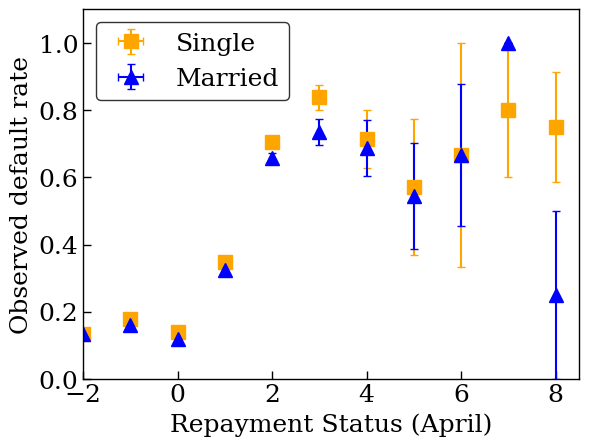
Case study #2: Credit Default
The second case study that we will consider in this tutorial is predicting an individual's credit default probability. We will use the Default of Credit Card Clients dataset from the UCI repository. This data was collected from 30,000 Taiwanese credit card users and contains a binary label of whether or not a user defaulted on a payment in a time window. Features include marital status, gender, education, and how long a user is behind on payment of their existing bills, for each of the months of April-September 2005.
As we did with the first case study, we again illustrate using monotonicity constraints to avoid unfair penalization: if the model were to be used to determine a user’s credit score, it could feel unfair to many if they were penalized for paying their bills sooner, all else equal. Thus, we apply a monotonicity constraint that keeps the model from penalizing early payments.
Load Credit Default data
# Load data file.
credit_file_name = 'credit_default.csv'
credit_file_path = os.path.join(DATA_DIR, credit_file_name)
credit_df = pd.read_csv(credit_file_path, delimiter=',')
# Define label column name.
CREDIT_LABEL = 'default'
Split data into train/validation/test sets
dfs = {}
datasets = {}

dfs["credit_train"], dfs["credit_val"], dfs["credit_test"] = split_dataset(
    credit_df
)

for df_name, df in dfs.items():
  datasets[df_name] = tf.data.Dataset.from_tensor_slices(
      ((df[['MARRIAGE']], df[['PAY_0']]), df[['default']])
  ).batch(BATCH_SIZE)
Visualize data distribution
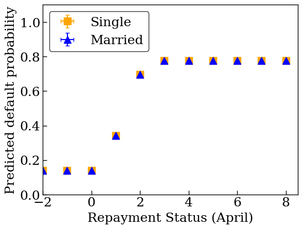
First we will visualize the distribution of the data. We will plot the mean and standard error of the observed default rate for people with different marital statuses and repayment statuses. The repayment status represents the number of months a person is behind on paying back their loan (as of April 2005).
def get_agg_data(df, x_col, y_col, bins=11):
  xbins = pd.cut(df[x_col], bins=bins)
  data = df[[x_col, y_col]].groupby(xbins).agg(['mean', 'sem'])
  return data


def plot_2d_means_credit(input_df, x_col, y_col, x_label, y_label):
  plt.rcParams['font.family'] = ['serif']
  _, ax = plt.subplots(nrows=1, ncols=1)
  plt.setp(ax.spines.values(), color='black', linewidth=1)
  ax.tick_params(
      direction='in', length=6, width=1, top=False, right=False, labelsize=18)
  df_single = get_agg_data(input_df[input_df['MARRIAGE'] == 1], x_col, y_col)
  df_married = get_agg_data(input_df[input_df['MARRIAGE'] == 2], x_col, y_col)
  ax.errorbar(
      df_single[(x_col, 'mean')],
      df_single[(y_col, 'mean')],
      xerr=df_single[(x_col, 'sem')],
      yerr=df_single[(y_col, 'sem')],
      color='orange',
      marker='s',
      capsize=3,
      capthick=1,
      label='Single',
      markersize=10,
      linestyle='')
  ax.errorbar(
      df_married[(x_col, 'mean')],
      df_married[(y_col, 'mean')],
      xerr=df_married[(x_col, 'sem')],
      yerr=df_married[(y_col, 'sem')],
      color='b',
      marker='^',
      capsize=3,
      capthick=1,
      label='Married',
      markersize=10,
      linestyle='')
  leg = ax.legend(loc='upper left', fontsize=18, frameon=True, numpoints=1)
  ax.set_xlabel(x_label, fontsize=18)
  ax.set_ylabel(y_label, fontsize=18)
  ax.set_ylim(0, 1.1)
  ax.set_xlim(-2, 8.5)
  ax.patch.set_facecolor('white')
  leg.get_frame().set_edgecolor('black')
  leg.get_frame().set_facecolor('white')
  leg.get_frame().set_linewidth(1)
  plt.show()
plot_2d_means_credit(
    dfs['credit_train'],
    'PAY_0',
    'default',
    'Repayment Status (April)',
    'Observed default rate',
)
/tmpfs/tmp/ipykernel_51492/4037607942.py:3: FutureWarning: The default of observed=False is deprecated and will be changed to True in a future version of pandas. Pass observed=False to retain current behavior or observed=True to adopt the future default and silence this warning.
  data = df[[x_col, y_col]].groupby(xbins).agg(['mean', 'sem'])
Train calibrated lattice model to predict credit default rate
Next, we will train a calibrated lattice model from TFL to predict whether or not a person will default on a loan. The two input features will be the person's marital status and how many months the person is behind on paying back their loans in April (repayment status). The training label will be whether or not the person defaulted on a loan.
We will first train a calibrated lattice model without any constraints. Then, we will train a calibrated lattice model with monotonicity constraints and observe the difference in the model output and accuracy.
Helper functions for visualization of trained model outputs
def plot_predictions_credit(
    input_df,
    model,
    x_col,
    x_label='Repayment Status (April)',
    y_label='Predicted default probability',
):
  predictions = model.predict((input_df[['MARRIAGE']], input_df[['PAY_0']]))
  predictions = tf.math.sigmoid(predictions)
  new_df = input_df.copy()
  new_df.loc[:, 'predictions'] = predictions
  plot_2d_means_credit(new_df, x_col, 'predictions', x_label, y_label)
Train unconstrained (non-monotonic) calibrated lattice model
model_config = tfl.configs.CalibratedLatticeConfig(
    feature_configs=[
        tfl.configs.FeatureConfig(
            name='MARRIAGE',
            lattice_size=3,
            pwl_calibration_num_keypoints=2,
            monotonicity=0,
            pwl_calibration_always_monotonic=False,
        ),
        tfl.configs.FeatureConfig(
            name='PAY_0',
            lattice_size=3,
            pwl_calibration_num_keypoints=16,
            monotonicity=0,
            pwl_calibration_always_monotonic=False,
        ),
    ],
    output_calibration=True,
    output_initialization=np.linspace(-2, 2, num=8),
)
feature_keypoints = tfl.premade_lib.compute_feature_keypoints(
    feature_configs=model_config.feature_configs,
    features=dfs["credit_train"][['MARRIAGE', 'PAY_0', 'default']],
)
tfl.premade_lib.set_feature_keypoints(
    feature_configs=model_config.feature_configs,
    feature_keypoints=feature_keypoints,
    add_missing_feature_configs=False,
)
nomon_lattice_model = tfl.premade.CalibratedLattice(model_config=model_config)

nomon_lattice_model.compile(
    loss=keras.losses.BinaryCrossentropy(from_logits=True),
    metrics=[
        keras.metrics.BinaryAccuracy(name='accuracy'),
    ],
    optimizer=keras.optimizers.Adam(LEARNING_RATES),
)
nomon_lattice_model.fit(datasets['credit_train'], epochs=NUM_EPOCHS, verbose=0)

train_acc = nomon_lattice_model.evaluate(datasets['credit_train'])[1]
val_acc = nomon_lattice_model.evaluate(datasets['credit_val'])[1]
test_acc = nomon_lattice_model.evaluate(datasets['credit_test'])[1]
print(
    'accuracies for train: %f, val: %f, test: %f'
    % (train_acc, val_acc, test_acc)
)
83/83 [==============================] - 0s 1ms/step - loss: 0.4537 - accuracy: 0.8186
12/12 [==============================] - 0s 2ms/step - loss: 0.4423 - accuracy: 0.8291
24/24 [==============================] - 0s 1ms/step - loss: 0.4547 - accuracy: 0.8168
accuracies for train: 0.818619, val: 0.829085, test: 0.816835
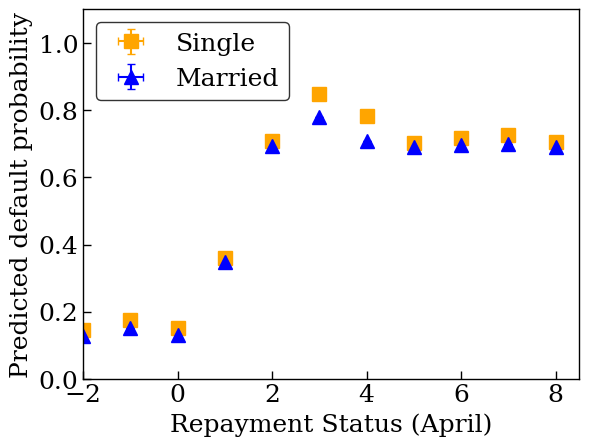
plot_predictions_credit(dfs['credit_train'], nomon_lattice_model, 'PAY_0')
657/657 [==============================] - 1s 1ms/step
/tmpfs/tmp/ipykernel_51492/4037607942.py:3: FutureWarning: The default of observed=False is deprecated and will be changed to True in a future version of pandas. Pass observed=False to retain current behavior or observed=True to adopt the future default and silence this warning.
  data = df[[x_col, y_col]].groupby(xbins).agg(['mean', 'sem'])
Train monotonic calibrated lattice model
model_config.feature_configs[0].monotonicity = 1
model_config.feature_configs[1].monotonicity = 1
mon_lattice_model = tfl.premade.CalibratedLattice(model_config=model_config)

mon_lattice_model.compile(
    loss=keras.losses.BinaryCrossentropy(from_logits=True),
    metrics=[
        keras.metrics.BinaryAccuracy(name='accuracy'),
    ],
    optimizer=keras.optimizers.Adam(LEARNING_RATES),
)
mon_lattice_model.fit(datasets['credit_train'], epochs=NUM_EPOCHS, verbose=0)

train_acc = mon_lattice_model.evaluate(datasets['credit_train'])[1]
val_acc = mon_lattice_model.evaluate(datasets['credit_val'])[1]
test_acc = mon_lattice_model.evaluate(datasets['credit_test'])[1]
print(
    'accuracies for train: %f, val: %f, test: %f'
    % (train_acc, val_acc, test_acc)
)
83/83 [==============================] - 0s 1ms/step - loss: 0.4548 - accuracy: 0.8188
12/12 [==============================] - 0s 2ms/step - loss: 0.4426 - accuracy: 0.8301
24/24 [==============================] - 0s 1ms/step - loss: 0.4551 - accuracy: 0.8172
accuracies for train: 0.818762, val: 0.830065, test: 0.817172
plot_predictions_credit(dfs['credit_train'], mon_lattice_model, 'PAY_0')
657/657 [==============================] - 1s 1ms/step
/tmpfs/tmp/ipykernel_51492/4037607942.py:3: FutureWarning: The default of observed=False is deprecated and will be changed to True in a future version of pandas. Pass observed=False to retain current behavior or observed=True to adopt the future default and silence this warning.
  data = df[[x_col, y_col]].groupby(xbins).agg(['mean', 'sem'])
/tmpfs/tmp/ipykernel_51492/4037607942.py:3: FutureWarning: The default of observed=False is deprecated and will be changed to True in a future version of pandas. Pass observed=False to retain current behavior or observed=True to adopt the future default and silence this warning.
  data = df[[x_col, y_col]].groupby(xbins).agg(['mean', 'sem'])