Adversarial regularization for image classification

View on TensorFlow.org

Run in Google Colab

View source on GitHub

Download notebook

Overview

In this tutorial, we will explore the use of adversarial learning (Goodfellow et al., 2014) for image classification using the Neural Structured Learning (NSL) framework.

The core idea of adversarial learning is to train a model with adversarially-perturbed data (called adversarial examples) in addition to the organic training data. To the human eye, these adversarial examples look the same as the original but the perturbation will cause the model to be confused and make incorrect predictions or classifications. The adversarial examples are constructed to intentionally mislead the model into making wrong predictions or classifications. By training with such examples, the model learns to be robust against adversarial perturbation when making predictions.

In this tutorial, we illustrate the following procedure of applying adversarial learning to obtain robust models using the Neural Structured Learning framework:

Create a neural network as a base model. In this tutorial, the base model is created with the tf.keras functional API; this procedure is compatible with models created by tf.keras sequential and subclassing APIs as well. For more information on Keras models in TensorFlow, see this documentation.
Wrap the base model with the AdversarialRegularization wrapper class, which is provided by the NSL framework, to create a new tf.keras.Model instance. This new model will include the adversarial loss as a regularization term in its training objective.
Convert examples in the training data to feature dictionaries.
Train and evaluate the new model.

Recap for Beginners

There is a corresponding video explanation on adversarial learning for image classification part of the TensorFlow Neural Structured Learning Youtube series. Below, we have summarized the key concepts explained in this video, expanding on the explanation provided in the Overview section above.

The NSL framework jointly optimizes both image features and structured signals to help neural networks better learn. However, what if there is no explicit structure available to train the neural network? This tutorial explains one approach involving the creation of adversarial neighbors (modified from the original sample) to dynamically construct a structure.

Firstly, adversarial neighbors are defined as modified versions of the sample image applied with small perturbations that mislead a neural net into outputting inaccurate classifications. These carefully designed perturbations are typically based on the reverse gradient direction and are meant to confuse the neural net during training. Humans may not be able to tell the difference between a sample image and it's generated adversarial neighbor. However, to the neural net, the applied perturbations are effective at leading to an inaccurate conclusion.

Generated adversarial neighbors are then connected to the sample, therefore dynamically constructing a structure edge by edge. Using this connection, neural nets learn to maintain the similarities between the sample and the adversarial neighbors while avoiding confusion resulting from misclassifications, thus improving the overall neural network's quality and accuracy.

The code segment below is a high-level explanation of the steps involved while the rest of this tutorial goes into further depth and technicality.

Read and prepare the data. Load the MNIST dataset and normalize the feature values to stay in the range [0,1]

import neural_structured_learning as nsl

(x_train, y_train), (x_train, y_train) = tf.keras.datasets.mnist.load_data()
x_train, x_test = x_train / 255.0, x_test / 255.0

Build the neural network. A Sequential Keras base model is used for this example.

model = tf.keras.Sequential(...)

Configure the adversarial model. Including the hyperparameters: multiplier applied on the adversarial regularization, empirically chosen differ values for step size/learning rate. Invoke adversarial regularization with a wrapper class around the constructed neural network.

adv_config = nsl.configs.make_adv_reg_config(multiplier=0.2, adv_step_size=0.05)
adv_model = nsl.keras.AdversarialRegularization(model, adv_config)

Conclude with the standard Keras workflow: compile, fit, evaluate.

adv_model.compile(optimizer='adam', loss='sparse_categorizal_crossentropy', metrics=['accuracy'])
adv_model.fit({'feature': x_train, 'label': y_train}, epochs=5)
adv_model.evaluate({'feature': x_test, 'label': y_test})

What you see here is adversarial learning enabled in 2 steps and 3 simple lines of code. This is the simplicity of the neural structured learning framework. In the following sections, we expand upon this procedure.

Setup

Install the Neural Structured Learning package.

pip install --quiet neural-structured-learning

Import libraries. We abbreviate neural_structured_learning to nsl.

import matplotlib.pyplot as plt
import neural_structured_learning as nsl
import numpy as np
import tensorflow as tf
import tensorflow_datasets as tfds

2023-10-03 11:17:25.316470: E tensorflow/compiler/xla/stream_executor/cuda/cuda_dnn.cc:9342] Unable to register cuDNN factory: Attempting to register factory for plugin cuDNN when one has already been registered
2023-10-03 11:17:25.316516: E tensorflow/compiler/xla/stream_executor/cuda/cuda_fft.cc:609] Unable to register cuFFT factory: Attempting to register factory for plugin cuFFT when one has already been registered
2023-10-03 11:17:25.316552: E tensorflow/compiler/xla/stream_executor/cuda/cuda_blas.cc:1518] Unable to register cuBLAS factory: Attempting to register factory for plugin cuBLAS when one has already been registered

Hyperparameters

We collect and explain the hyperparameters (in an HParams object) for model training and evaluation.

Input/Output:

input_shape: The shape of the input tensor. Each image is 28-by-28 pixels with 1 channel.
num_classes: There are a total of 10 classes, corresponding to 10 digits [0-9].

Model architecture:

conv_filters: A list of numbers, each specifying the number of filters in a convolutional layer.
kernel_size: The size of 2D convolution window, shared by all convolutional layers.
pool_size: Factors to downscale the image in each max-pooling layer.
num_fc_units: The number of units (i.e., width) of each fully-connected layer.

Training and evaluation:

batch_size: Batch size used for training and evaluation.
epochs: The number of training epochs.

Adversarial learning:

adv_multiplier: The weight of adversarial loss in the training objective, relative to the labeled loss.
adv_step_size: The magnitude of adversarial perturbation.
adv_grad_norm: The norm to measure the magnitude of adversarial perturbation.

class HParams(object):
  def __init__(self):
    self.input_shape = [28, 28, 1]
    self.num_classes = 10
    self.conv_filters = [32, 64, 64]
    self.kernel_size = (3, 3)
    self.pool_size = (2, 2)
    self.num_fc_units = [64]
    self.batch_size = 32
    self.epochs = 5
    self.adv_multiplier = 0.2
    self.adv_step_size = 0.2
    self.adv_grad_norm = 'infinity'

HPARAMS = HParams()

MNIST dataset

The MNIST dataset contains grayscale images of handwritten digits (from '0' to '9'). Each image shows one digit at low resolution (28-by-28 pixels). The task involved is to classify images into 10 categories, one per digit.

Here we load the MNIST dataset from TensorFlow Datasets. It handles downloading the data and constructing a tf.data.Dataset. The loaded dataset has two subsets:

train with 60,000 examples, and
test with 10,000 examples.

Examples in both subsets are stored in feature dictionaries with the following two keys:

image: Array of pixel values, ranging from 0 to 255.
label: Groundtruth label, ranging from 0 to 9.

datasets = tfds.load('mnist')

train_dataset = datasets['train']
test_dataset = datasets['test']

IMAGE_INPUT_NAME = 'image'
LABEL_INPUT_NAME = 'label'

2023-10-03 11:17:28.523912: E tensorflow/compiler/xla/stream_executor/cuda/cuda_driver.cc:268] failed call to cuInit: CUDA_ERROR_NO_DEVICE: no CUDA-capable device is detected

To make the model numerically stable, we normalize the pixel values to [0, 1] by mapping the dataset over the normalize function. After shuffling training set and batching, we convert the examples to feature tuples (image, label) for training the base model. We also provide a function to convert from tuples to dictionaries for later use.

def normalize(features):
  features[IMAGE_INPUT_NAME] = tf.cast(
      features[IMAGE_INPUT_NAME], dtype=tf.float32) / 255.0
  return features

def convert_to_tuples(features):
  return features[IMAGE_INPUT_NAME], features[LABEL_INPUT_NAME]

def convert_to_dictionaries(image, label):
  return {IMAGE_INPUT_NAME: image, LABEL_INPUT_NAME: label}

train_dataset = train_dataset.map(normalize).shuffle(10000).batch(HPARAMS.batch_size).map(convert_to_tuples)
test_dataset = test_dataset.map(normalize).batch(HPARAMS.batch_size).map(convert_to_tuples)

Base model

Our base model will be a neural network consisting of 3 convolutional layers follwed by 2 fully-connected layers (as defined in HPARAMS). Here we define it using the Keras functional API. Feel free to try other APIs or model architectures (e.g. subclassing). Note that the NSL framework does support all three types of Keras APIs.

def build_base_model(hparams):
  """Builds a model according to the architecture defined in `hparams`."""
  inputs = tf.keras.Input(
      shape=hparams.input_shape, dtype=tf.float32, name=IMAGE_INPUT_NAME)

  x = inputs
  for i, num_filters in enumerate(hparams.conv_filters):
    x = tf.keras.layers.Conv2D(
        num_filters, hparams.kernel_size, activation='relu')(
            x)
    if i < len(hparams.conv_filters) - 1:
      # max pooling between convolutional layers
      x = tf.keras.layers.MaxPooling2D(hparams.pool_size)(x)
  x = tf.keras.layers.Flatten()(x)
  for num_units in hparams.num_fc_units:
    x = tf.keras.layers.Dense(num_units, activation='relu')(x)
  pred = tf.keras.layers.Dense(hparams.num_classes)(x)
  model = tf.keras.Model(inputs=inputs, outputs=pred)
  return model

base_model = build_base_model(HPARAMS)
base_model.summary()

Model: "model"
_________________________________________________________________
 Layer (type)                Output Shape              Param #   
=================================================================
 image (InputLayer)          [(None, 28, 28, 1)]       0         
                                                                 
 conv2d (Conv2D)             (None, 26, 26, 32)        320       
                                                                 
 max_pooling2d (MaxPooling2  (None, 13, 13, 32)        0         
 D)                                                              
                                                                 
 conv2d_1 (Conv2D)           (None, 11, 11, 64)        18496     
                                                                 
 max_pooling2d_1 (MaxPoolin  (None, 5, 5, 64)          0         
 g2D)                                                            
                                                                 
 conv2d_2 (Conv2D)           (None, 3, 3, 64)          36928     
                                                                 
 flatten (Flatten)           (None, 576)               0         
                                                                 
 dense (Dense)               (None, 64)                36928     
                                                                 
 dense_1 (Dense)             (None, 10)                650       
                                                                 
=================================================================
Total params: 93322 (364.54 KB)
Trainable params: 93322 (364.54 KB)
Non-trainable params: 0 (0.00 Byte)
_________________________________________________________________

Next we train and evaluate the base model.

base_model.compile(
    optimizer='adam',
    loss=tf.keras.losses.SparseCategoricalCrossentropy(from_logits=True),
    metrics=['acc'])
base_model.fit(train_dataset, epochs=HPARAMS.epochs)

Epoch 1/5
1875/1875 [==============================] - 15s 7ms/step - loss: 0.1421 - acc: 0.9570
Epoch 2/5
1875/1875 [==============================] - 13s 7ms/step - loss: 0.0459 - acc: 0.9862
Epoch 3/5
1875/1875 [==============================] - 13s 7ms/step - loss: 0.0327 - acc: 0.9897
Epoch 4/5
1875/1875 [==============================] - 13s 7ms/step - loss: 0.0240 - acc: 0.9923
Epoch 5/5
1875/1875 [==============================] - 13s 7ms/step - loss: 0.0204 - acc: 0.9934
<keras.src.callbacks.History at 0x7f822f65a2e0>

results = base_model.evaluate(test_dataset)
named_results = dict(zip(base_model.metrics_names, results))
print('\naccuracy:', named_results['acc'])

313/313 [==============================] - 1s 3ms/step - loss: 0.0261 - acc: 0.9918

accuracy: 0.9918000102043152

We can see that the base model achieves 99% accuracy on the test set. We will see how robust it is in Robustness Under Adversarial Perturbations below.

Adversarial-regularized model

Here we show how to incorporate adversarial training into a Keras model with a few lines of code, using the NSL framework. The base model is wrapped to create a new tf.Keras.Model, whose training objective includes adversarial regularization.

First, we create a config object with all relevant hyperparameters using the helper function nsl.configs.make_adv_reg_config.

adv_config = nsl.configs.make_adv_reg_config(
    multiplier=HPARAMS.adv_multiplier,
    adv_step_size=HPARAMS.adv_step_size,
    adv_grad_norm=HPARAMS.adv_grad_norm
)

Now we can wrap a base model with AdversarialRegularization. Here we create a new base model (base_adv_model), so that the existing one (base_model) can be used in later comparison.

The returned adv_model is a tf.keras.Model object, whose training objective includes a regularization term for the adversarial loss. To compute that loss, the model has to have access to the label information (feature label), in addition to regular input (feature image). For this reason, we convert the examples in the datasets from tuples back to dictionaries. And we tell the model which feature contains the label information via the label_keys parameter.

base_adv_model = build_base_model(HPARAMS)
adv_model = nsl.keras.AdversarialRegularization(
    base_adv_model,
    label_keys=[LABEL_INPUT_NAME],
    adv_config=adv_config
)

train_set_for_adv_model = train_dataset.map(convert_to_dictionaries)
test_set_for_adv_model = test_dataset.map(convert_to_dictionaries)

Next we compile, train, and evaluate the adversarial-regularized model. There might be warnings like "Output missing from loss dictionary," which is fine because the adv_model doesn't rely on the base implementation to calculate the total loss.

adv_model.compile(
    optimizer='adam',
    loss=tf.keras.losses.SparseCategoricalCrossentropy(from_logits=True),
    metrics=['acc'])
adv_model.fit(train_set_for_adv_model, epochs=HPARAMS.epochs)

Epoch 1/5
WARNING:absl:Cannot perturb non-Tensor input: dict_keys(['label'])
1875/1875 [==============================] - 24s 11ms/step - loss: 0.2940 - sparse_categorical_crossentropy: 0.1341 - sparse_categorical_accuracy: 0.9598 - scaled_adversarial_loss: 0.1599
Epoch 2/5
1875/1875 [==============================] - 21s 11ms/step - loss: 0.1231 - sparse_categorical_crossentropy: 0.0403 - sparse_categorical_accuracy: 0.9872 - scaled_adversarial_loss: 0.0827
Epoch 3/5
1875/1875 [==============================] - 21s 11ms/step - loss: 0.0875 - sparse_categorical_crossentropy: 0.0266 - sparse_categorical_accuracy: 0.9917 - scaled_adversarial_loss: 0.0609
Epoch 4/5
1875/1875 [==============================] - 21s 11ms/step - loss: 0.0711 - sparse_categorical_crossentropy: 0.0222 - sparse_categorical_accuracy: 0.9930 - scaled_adversarial_loss: 0.0489
Epoch 5/5
1875/1875 [==============================] - 21s 11ms/step - loss: 0.0545 - sparse_categorical_crossentropy: 0.0163 - sparse_categorical_accuracy: 0.9947 - scaled_adversarial_loss: 0.0382
<keras.src.callbacks.History at 0x7f814416dbe0>

results = adv_model.evaluate(test_set_for_adv_model)
named_results = dict(zip(adv_model.metrics_names, results))
print('\naccuracy:', named_results['sparse_categorical_accuracy'])

313/313 [==============================] - 2s 6ms/step - loss: 0.0704 - sparse_categorical_crossentropy: 0.0312 - sparse_categorical_accuracy: 0.9898 - scaled_adversarial_loss: 0.0392

accuracy: 0.989799976348877

We can see that the adversarial-regularized model also performs very well (99% accuracy) on the test set.

Robustness under Adversarial perturbations

Now we compare the base model and the adversarial-regularized model for robustness under adversarial perturbation.

We will use the AdversarialRegularization.perturb_on_batch function for generating adversarially perturbed examples. And we would like the generation based on the base model. To do so, we wrap the base model with AdversarialRegularization. Note that as long as we don't invoke training (Model.fit), the learned variables in the model won't change and the model is still the same one as in section Base Model.

reference_model = nsl.keras.AdversarialRegularization(
    base_model, label_keys=[LABEL_INPUT_NAME], adv_config=adv_config)
reference_model.compile(
    optimizer='adam',
    loss=tf.keras.losses.SparseCategoricalCrossentropy(from_logits=True),
    metrics=['acc'])

We collect in a dictionary the models to be evaluted, and also create a metric object for each of the models.

Note that we take adv_model.base_model in order to have the same input format (not requiring label information) as the base model. The learned variables in adv_model.base_model are the same as those in adv_model.

models_to_eval = {
    'base': base_model,
    'adv-regularized': adv_model.base_model
}
metrics = {
    name: tf.keras.metrics.SparseCategoricalAccuracy()
    for name in models_to_eval.keys()
}

Here is the loop to generate perturbed examples and to evaluate models with them. We save the perturbed images, labels, and predictions for visualization in the next section.

perturbed_images, labels, predictions = [], [], []

for batch in test_set_for_adv_model:
  perturbed_batch = reference_model.perturb_on_batch(batch)
  # Clipping makes perturbed examples have the same range as regular ones.
  perturbed_batch[IMAGE_INPUT_NAME] = tf.clip_by_value(
      perturbed_batch[IMAGE_INPUT_NAME], 0.0, 1.0)
  y_true = perturbed_batch.pop(LABEL_INPUT_NAME)
  perturbed_images.append(perturbed_batch[IMAGE_INPUT_NAME].numpy())
  labels.append(y_true.numpy())
  predictions.append({})
  for name, model in models_to_eval.items():
    y_pred = model(perturbed_batch)
    metrics[name](y_true, y_pred)
    predictions[-1][name] = tf.argmax(y_pred, axis=-1).numpy()

for name, metric in metrics.items():
  print('%s model accuracy: %f' % (name, metric.result().numpy()))

WARNING:absl:Cannot perturb non-Tensor input: dict_keys(['label'])
base model accuracy: 0.514900
adv-regularized model accuracy: 0.951000

We can see that the accuracy of the base model drops dramatically (from 99% to about 50%) when the input is perturbed adversarially. On the other hand, the accuracy of the adversarial-regularized model only degrades a little (from 99% to 95%). This demonstrates the effectiveness of adversarial learning on improving model's robustness.

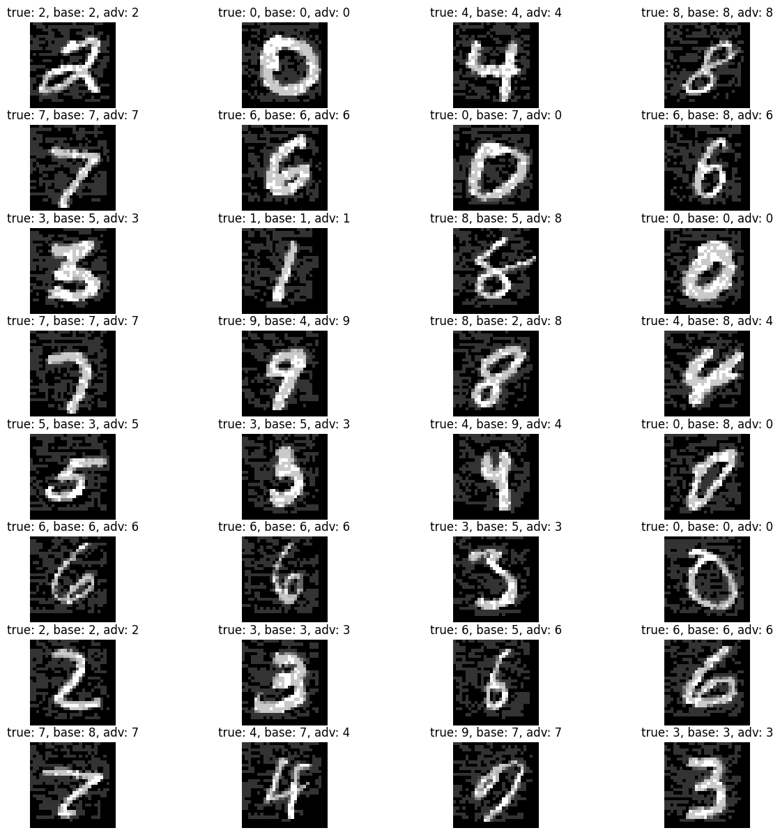
Examples of adversarially-perturbed images

Here we take a look at the adversarially-perturbed images. We can see that the perturbed images still show digits recognizable by human, but can successfully fool the base model.

batch_index = 0

batch_image = perturbed_images[batch_index]
batch_label = labels[batch_index]
batch_pred = predictions[batch_index]

batch_size = HPARAMS.batch_size
n_col = 4
n_row = (batch_size + n_col - 1) // n_col

print('accuracy in batch %d:' % batch_index)
for name, pred in batch_pred.items():
  print('%s model: %d / %d' % (name, np.sum(batch_label == pred), batch_size))

plt.figure(figsize=(15, 15))
for i, (image, y) in enumerate(zip(batch_image, batch_label)):
  y_base = batch_pred['base'][i]
  y_adv = batch_pred['adv-regularized'][i]
  plt.subplot(n_row, n_col, i+1)
  plt.title('true: %d, base: %d, adv: %d' % (y, y_base, y_adv))
  plt.imshow(tf.keras.utils.array_to_img(image), cmap='gray')
  plt.axis('off')

plt.show()

accuracy in batch 0:
base model: 16 / 32
adv-regularized model: 31 / 32

png

Conclusion

We have demonstrated the use of adversarial learning for image classification using the Neural Structured Learning (NSL) framework. We encourage users to experiment with different adversarial settings (in hyper-parameters) and to see how they affect model robustness.