
|
|
|
 View source on GitHub View source on GitHub
|
|
|
Overview
This notebook classifies movie reviews as positive or negative using the text of the review. This is an example of binary classification, an important and widely applicable kind of machine learning problem.
We will demonstrate the use of graph regularization in this notebook by building a graph from the given input. The general recipe for building a graph-regularized model using the Neural Structured Learning (NSL) framework when the input does not contain an explicit graph is as follows:
- Create embeddings for each text sample in the input. This can be done using pre-trained models such as word2vec, Swivel, BERT etc.
- Build a graph based on these embeddings by using a similarity metric such as the 'L2' distance, 'cosine' distance, etc. Nodes in the graph correspond to samples and edges in the graph correspond to similarity between pairs of samples.
- Generate training data from the above synthesized graph and sample features. The resulting training data will contain neighbor features in addition to the original node features.
- Create a neural network as a base model using the Keras sequential, functional, or subclass API.
- Wrap the base model with the GraphRegularization wrapper class, which is provided by the NSL framework, to create a new graph Keras model. This new model will include a graph regularization loss as the regularization term in its training objective.
- Train and evaluate the graph Keras model.
Requirements
- Install the Neural Structured Learning package.
- Install tensorflow-hub.
pip install --quiet neural-structured-learningpip install --quiet tensorflow-hub
Dependencies and imports
import matplotlib.pyplot as plt
import numpy as np

import neural_structured_learning as nsl

import tensorflow as tf
import tensorflow_hub as hub

# Resets notebook state
tf.keras.backend.clear_session()

print("Version: ", tf.__version__)
print("Eager mode: ", tf.executing_eagerly())
print("Hub version: ", hub.__version__)
print(
    "GPU is",
    "available" if tf.config.list_physical_devices("GPU") else "NOT AVAILABLE")
2022-12-14 12:19:13.551836: W tensorflow/compiler/xla/stream_executor/platform/default/dso_loader.cc:64] Could not load dynamic library 'libnvinfer.so.7'; dlerror: libnvinfer.so.7: cannot open shared object file: No such file or directory
2022-12-14 12:19:13.551949: W tensorflow/compiler/xla/stream_executor/platform/default/dso_loader.cc:64] Could not load dynamic library 'libnvinfer_plugin.so.7'; dlerror: libnvinfer_plugin.so.7: cannot open shared object file: No such file or directory
2022-12-14 12:19:13.551962: W tensorflow/compiler/tf2tensorrt/utils/py_utils.cc:38] TF-TRT Warning: Cannot dlopen some TensorRT libraries. If you would like to use Nvidia GPU with TensorRT, please make sure the missing libraries mentioned above are installed properly.
Version:  2.11.0
Eager mode:  True
Hub version:  0.12.0
GPU is NOT AVAILABLE
2022-12-14 12:19:14.770677: E tensorflow/compiler/xla/stream_executor/cuda/cuda_driver.cc:267] failed call to cuInit: CUDA_ERROR_NO_DEVICE: no CUDA-capable device is detected
IMDB dataset
The IMDB dataset contains the text of 50,000 movie reviews from the Internet Movie Database. These are split into 25,000 reviews for training and 25,000 reviews for testing. The training and testing sets are balanced, meaning they contain an equal number of positive and negative reviews.
In this tutorial, we will use a preprocessed version of the IMDB dataset.
Download preprocessed IMDB dataset
The IMDB dataset comes packaged with TensorFlow. It has already been preprocessed such that the reviews (sequences of words) have been converted to sequences of integers, where each integer represents a specific word in a dictionary.
The following code downloads the IMDB dataset (or uses a cached copy if it has already been downloaded):
imdb = tf.keras.datasets.imdb
(pp_train_data, pp_train_labels), (pp_test_data, pp_test_labels) = (
    imdb.load_data(num_words=10000))
Downloading data from https://storage.googleapis.com/tensorflow/tf-keras-datasets/imdb.npz
17464789/17464789 [==============================] - 0s 0us/step
The argument num_words=10000 keeps the top 10,000 most frequently occurring words in the training data. The rare words are discarded to keep the size of the vocabulary manageable.
Explore the data
Let's take a moment to understand the format of the data. The dataset comes preprocessed: each example is an array of integers representing the words of the movie review. Each label is an integer value of either 0 or 1, where 0 is a negative review, and 1 is a positive review.
print('Training entries: {}, labels: {}'.format(
    len(pp_train_data), len(pp_train_labels)))
training_samples_count = len(pp_train_data)
Training entries: 25000, labels: 25000
The text of reviews have been converted to integers, where each integer represents a specific word in a dictionary. Here's what the first review looks like:
print(pp_train_data[0])
[1, 14, 22, 16, 43, 530, 973, 1622, 1385, 65, 458, 4468, 66, 3941, 4, 173, 36, 256, 5, 25, 100, 43, 838, 112, 50, 670, 2, 9, 35, 480, 284, 5, 150, 4, 172, 112, 167, 2, 336, 385, 39, 4, 172, 4536, 1111, 17, 546, 38, 13, 447, 4, 192, 50, 16, 6, 147, 2025, 19, 14, 22, 4, 1920, 4613, 469, 4, 22, 71, 87, 12, 16, 43, 530, 38, 76, 15, 13, 1247, 4, 22, 17, 515, 17, 12, 16, 626, 18, 2, 5, 62, 386, 12, 8, 316, 8, 106, 5, 4, 2223, 5244, 16, 480, 66, 3785, 33, 4, 130, 12, 16, 38, 619, 5, 25, 124, 51, 36, 135, 48, 25, 1415, 33, 6, 22, 12, 215, 28, 77, 52, 5, 14, 407, 16, 82, 2, 8, 4, 107, 117, 5952, 15, 256, 4, 2, 7, 3766, 5, 723, 36, 71, 43, 530, 476, 26, 400, 317, 46, 7, 4, 2, 1029, 13, 104, 88, 4, 381, 15, 297, 98, 32, 2071, 56, 26, 141, 6, 194, 7486, 18, 4, 226, 22, 21, 134, 476, 26, 480, 5, 144, 30, 5535, 18, 51, 36, 28, 224, 92, 25, 104, 4, 226, 65, 16, 38, 1334, 88, 12, 16, 283, 5, 16, 4472, 113, 103, 32, 15, 16, 5345, 19, 178, 32]
Movie reviews may be different lengths. The below code shows the number of words in the first and second reviews. Since inputs to a neural network must be the same length, we'll need to resolve this later.
len(pp_train_data[0]), len(pp_train_data[1])
(218, 189)
Convert the integers back to words
It may be useful to know how to convert integers back to the corresponding text. Here, we'll create a helper function to query a dictionary object that contains the integer to string mapping:
def build_reverse_word_index():
  # A dictionary mapping words to an integer index
  word_index = imdb.get_word_index()

  # The first indices are reserved
  word_index = {k: (v + 3) for k, v in word_index.items()}
  word_index['<PAD>'] = 0
  word_index['<START>'] = 1
  word_index['<UNK>'] = 2  # unknown
  word_index['<UNUSED>'] = 3
  return dict((value, key) for (key, value) in word_index.items())

reverse_word_index = build_reverse_word_index()

def decode_review(text):
  return ' '.join([reverse_word_index.get(i, '?') for i in text])
Downloading data from https://storage.googleapis.com/tensorflow/tf-keras-datasets/imdb_word_index.json
1641221/1641221 [==============================] - 0s 0us/step
Now we can use the decode_review function to display the text for the first review:
decode_review(pp_train_data[0])
"<START> this film was just brilliant casting location scenery story direction everyone's really suited the part they played and you could just imagine being there robert <UNK> is an amazing actor and now the same being director <UNK> father came from the same scottish island as myself so i loved the fact there was a real connection with this film the witty remarks throughout the film were great it was just brilliant so much that i bought the film as soon as it was released for <UNK> and would recommend it to everyone to watch and the fly fishing was amazing really cried at the end it was so sad and you know what they say if you cry at a film it must have been good and this definitely was also <UNK> to the two little boy's that played the <UNK> of norman and paul they were just brilliant children are often left out of the <UNK> list i think because the stars that play them all grown up are such a big profile for the whole film but these children are amazing and should be praised for what they have done don't you think the whole story was so lovely because it was true and was someone's life after all that was shared with us all"
Graph construction
Graph construction involves creating embeddings for text samples and then using a similarity function to compare the embeddings.
Before proceeding further, we first create a directory to store artifacts created by this tutorial.
mkdir -p /tmp/imdbCreate sample embeddings
We will use pretrained Swivel embeddings to create embeddings in the
tf.train.Example format for each sample in the input. We will store the
resulting embeddings in the TFRecord format along with an additional feature
that represents the ID of each sample. This is important and will allow us match
sample embeddings with corresponding nodes in the graph later.
pretrained_embedding = 'https://tfhub.dev/google/tf2-preview/gnews-swivel-20dim/1'

hub_layer = hub.KerasLayer(
    pretrained_embedding, input_shape=[], dtype=tf.string, trainable=True)
WARNING:tensorflow:Please fix your imports. Module tensorflow.python.training.tracking.data_structures has been moved to tensorflow.python.trackable.data_structures. The old module will be deleted in version 2.11.
def _int64_feature(value):
  """Returns int64 tf.train.Feature."""
  return tf.train.Feature(int64_list=tf.train.Int64List(value=value.tolist()))


def _bytes_feature(value):
  """Returns bytes tf.train.Feature."""
  return tf.train.Feature(
      bytes_list=tf.train.BytesList(value=[value.encode('utf-8')]))


def _float_feature(value):
  """Returns float tf.train.Feature."""
  return tf.train.Feature(float_list=tf.train.FloatList(value=value.tolist()))


def create_embedding_example(word_vector, record_id):
  """Create tf.Example containing the sample's embedding and its ID."""

  text = decode_review(word_vector)

  # Shape = [batch_size,].
  sentence_embedding = hub_layer(tf.reshape(text, shape=[-1,]))

  # Flatten the sentence embedding back to 1-D.
  sentence_embedding = tf.reshape(sentence_embedding, shape=[-1])

  features = {
      'id': _bytes_feature(str(record_id)),
      'embedding': _float_feature(sentence_embedding.numpy())
  }
  return tf.train.Example(features=tf.train.Features(feature=features))


def create_embeddings(word_vectors, output_path, starting_record_id):
  record_id = int(starting_record_id)
  with tf.io.TFRecordWriter(output_path) as writer:
    for word_vector in word_vectors:
      example = create_embedding_example(word_vector, record_id)
      record_id = record_id + 1
      writer.write(example.SerializeToString())
  return record_id


# Persist TF.Example features containing embeddings for training data in
# TFRecord format.
create_embeddings(pp_train_data, '/tmp/imdb/embeddings.tfr', 0)
25000
Build a graph
Now that we have the sample embeddings, we will use them to build a similarity graph, i.e, nodes in this graph will correspond to samples and edges in this graph will correspond to similarity between pairs of nodes.
Neural Structured Learning provides a graph building library to build a graph
based on sample embeddings. It uses
cosine similarity as the
similarity measure to compare embeddings and build edges between them. It also
allows us to specify a similarity threshold, which can be used to discard
dissimilar edges from the final graph. In this example, using 0.99 as the
similarity threshold and 12345 as the random seed, we end up with a graph that
has 429,415 bi-directional edges. Here we're using the graph builder's support
for locality-sensitive hashing
(LSH) to speed up graph building. For details on using the graph builder's LSH
support, see the
build_graph_from_config
API documentation.
graph_builder_config = nsl.configs.GraphBuilderConfig(
    similarity_threshold=0.99, lsh_splits=32, lsh_rounds=15, random_seed=12345)
nsl.tools.build_graph_from_config(['/tmp/imdb/embeddings.tfr'],
                                  '/tmp/imdb/graph_99.tsv',
                                  graph_builder_config)
Each bi-directional edge is represented by two directed edges in the output TSV file, so that file contains 429,415 * 2 = 858,830 total lines:
wc -l /tmp/imdb/graph_99.tsv858830 /tmp/imdb/graph_99.tsv
Sample features
We create sample features for our problem using the tf.train.Example format
and persist them in the TFRecord format. Each sample will include the
following three features:
- id: The node ID of the sample.
- words: An int64 list containing word IDs.
- label: A singleton int64 identifying the target class of the review.
def create_example(word_vector, label, record_id):
  """Create tf.Example containing the sample's word vector, label, and ID."""
  features = {
      'id': _bytes_feature(str(record_id)),
      'words': _int64_feature(np.asarray(word_vector)),
      'label': _int64_feature(np.asarray([label])),
  }
  return tf.train.Example(features=tf.train.Features(feature=features))

def create_records(word_vectors, labels, record_path, starting_record_id):
  record_id = int(starting_record_id)
  with tf.io.TFRecordWriter(record_path) as writer:
    for word_vector, label in zip(word_vectors, labels):
      example = create_example(word_vector, label, record_id)
      record_id = record_id + 1
      writer.write(example.SerializeToString())
  return record_id

# Persist TF.Example features (word vectors and labels) for training and test
# data in TFRecord format.
next_record_id = create_records(pp_train_data, pp_train_labels,
                                '/tmp/imdb/train_data.tfr', 0)
create_records(pp_test_data, pp_test_labels, '/tmp/imdb/test_data.tfr',
               next_record_id)
50000
Augment training data with graph neighbors
Since we have the sample features and the synthesized graph, we can generate the augmented training data for Neural Structured Learning. The NSL framework provides a library to combine the graph and the sample features to produce the final training data for graph regularization. The resulting training data will include original sample features as well as features of their corresponding neighbors.
In this tutorial, we consider undirected edges and use a maximum of 3 neighbors per sample to augment training data with graph neighbors.
nsl.tools.pack_nbrs(
    '/tmp/imdb/train_data.tfr',
    '',
    '/tmp/imdb/graph_99.tsv',
    '/tmp/imdb/nsl_train_data.tfr',
    add_undirected_edges=True,
    max_nbrs=3)
Base model
We are now ready to build a base model without graph regularization. In order to build this model, we can either use embeddings that were used in building the graph, or we can learn new embeddings jointly along with the classification task. For the purpose of this notebook, we will do the latter.
Global variables
NBR_FEATURE_PREFIX = 'NL_nbr_'
NBR_WEIGHT_SUFFIX = '_weight'
Hyperparameters
We will use an instance of HParams to inclue various hyperparameters and
constants used for training and evaluation. We briefly describe each of them
below:
num_classes: There are 2 classes -- positive and negative.
max_seq_length: This is the maximum number of words considered from each movie review in this example.
vocab_size: This is the size of the vocabulary considered for this example.
distance_type: This is the distance metric used to regularize the sample with its neighbors.
graph_regularization_multiplier: This controls the relative weight of the graph regularization term in the overall loss function.
num_neighbors: The number of neighbors used for graph regularization. This value has to be less than or equal to the
max_nbrsargument used above when invokingnsl.tools.pack_nbrs.num_fc_units: The number of units in the fully connected layer of the neural network.
train_epochs: The number of training epochs.
batch_size: Batch size used for training and evaluation.
eval_steps: The number of batches to process before deeming evaluation is complete. If set to
None, all instances in the test set are evaluated.
class HParams(object):
  """Hyperparameters used for training."""
  def __init__(self):
    ### dataset parameters
    self.num_classes = 2
    self.max_seq_length = 256
    self.vocab_size = 10000
    ### neural graph learning parameters
    self.distance_type = nsl.configs.DistanceType.L2
    self.graph_regularization_multiplier = 0.1
    self.num_neighbors = 2
    ### model architecture
    self.num_embedding_dims = 16
    self.num_lstm_dims = 64
    self.num_fc_units = 64
    ### training parameters
    self.train_epochs = 10
    self.batch_size = 128
    ### eval parameters
    self.eval_steps = None  # All instances in the test set are evaluated.

HPARAMS = HParams()
Prepare the data
The reviews—the arrays of integers—must be converted to tensors before being fed into the neural network. This conversion can be done a couple of ways:
Convert the arrays into vectors of
0s and1s indicating word occurrence, similar to a one-hot encoding. For example, the sequence[3, 5]would become a10000-dimensional vector that is all zeros except for indices3and5, which are ones. Then, make this the first layer in our network—aDenselayer—that can handle floating point vector data. This approach is memory intensive, though, requiring anum_words * num_reviewssize matrix.Alternatively, we can pad the arrays so they all have the same length, then create an integer tensor of shape
max_length * num_reviews. We can use an embedding layer capable of handling this shape as the first layer in our network.
In this tutorial, we will use the second approach.
Since the movie reviews must be the same length, we will use the pad_sequence
function defined below to standardize the lengths.
def make_dataset(file_path, training=False):
  """Creates a `tf.data.TFRecordDataset`.

  Args:
    file_path: Name of the file in the `.tfrecord` format containing
      `tf.train.Example` objects.
    training: Boolean indicating if we are in training mode.

  Returns:
    An instance of `tf.data.TFRecordDataset` containing the `tf.train.Example`
    objects.
  """

  def pad_sequence(sequence, max_seq_length):
    """Pads the input sequence (a `tf.SparseTensor`) to `max_seq_length`."""
    pad_size = tf.maximum([0], max_seq_length - tf.shape(sequence)[0])
    padded = tf.concat(
        [sequence.values,
         tf.fill((pad_size), tf.cast(0, sequence.dtype))],
        axis=0)
    # The input sequence may be larger than max_seq_length. Truncate down if
    # necessary.
    return tf.slice(padded, [0], [max_seq_length])

  def parse_example(example_proto):
    """Extracts relevant fields from the `example_proto`.

    Args:
      example_proto: An instance of `tf.train.Example`.

    Returns:
      A pair whose first value is a dictionary containing relevant features
      and whose second value contains the ground truth labels.
    """
    # The 'words' feature is a variable length word ID vector.
    feature_spec = {
        'words': tf.io.VarLenFeature(tf.int64),
        'label': tf.io.FixedLenFeature((), tf.int64, default_value=-1),
    }
    # We also extract corresponding neighbor features in a similar manner to
    # the features above during training.
    if training:
      for i in range(HPARAMS.num_neighbors):
        nbr_feature_key = '{}{}_{}'.format(NBR_FEATURE_PREFIX, i, 'words')
        nbr_weight_key = '{}{}{}'.format(NBR_FEATURE_PREFIX, i,
                                         NBR_WEIGHT_SUFFIX)
        feature_spec[nbr_feature_key] = tf.io.VarLenFeature(tf.int64)

        # We assign a default value of 0.0 for the neighbor weight so that
        # graph regularization is done on samples based on their exact number
        # of neighbors. In other words, non-existent neighbors are discounted.
        feature_spec[nbr_weight_key] = tf.io.FixedLenFeature(
            [1], tf.float32, default_value=tf.constant([0.0]))

    features = tf.io.parse_single_example(example_proto, feature_spec)

    # Since the 'words' feature is a variable length word vector, we pad it to a
    # constant maximum length based on HPARAMS.max_seq_length
    features['words'] = pad_sequence(features['words'], HPARAMS.max_seq_length)
    if training:
      for i in range(HPARAMS.num_neighbors):
        nbr_feature_key = '{}{}_{}'.format(NBR_FEATURE_PREFIX, i, 'words')
        features[nbr_feature_key] = pad_sequence(features[nbr_feature_key],
                                                 HPARAMS.max_seq_length)

    labels = features.pop('label')
    return features, labels

  dataset = tf.data.TFRecordDataset([file_path])
  if training:
    dataset = dataset.shuffle(10000)
  dataset = dataset.map(parse_example)
  dataset = dataset.batch(HPARAMS.batch_size)
  return dataset


train_dataset = make_dataset('/tmp/imdb/nsl_train_data.tfr', True)
test_dataset = make_dataset('/tmp/imdb/test_data.tfr')
Build the model
A neural network is created by stacking layers—this requires two main architectural decisions:
- How many layers to use in the model?
- How many hidden units to use for each layer?
In this example, the input data consists of an array of word-indices. The labels to predict are either 0 or 1.
We will use a bi-directional LSTM as our base model in this tutorial.
# This function exists as an alternative to the bi-LSTM model used in this
# notebook.
def make_feed_forward_model():
  """Builds a simple 2 layer feed forward neural network."""
  inputs = tf.keras.Input(
      shape=(HPARAMS.max_seq_length,), dtype='int64', name='words')
  embedding_layer = tf.keras.layers.Embedding(HPARAMS.vocab_size, 16)(inputs)
  pooling_layer = tf.keras.layers.GlobalAveragePooling1D()(embedding_layer)
  dense_layer = tf.keras.layers.Dense(16, activation='relu')(pooling_layer)
  outputs = tf.keras.layers.Dense(1)(dense_layer)
  return tf.keras.Model(inputs=inputs, outputs=outputs)


def make_bilstm_model():
  """Builds a bi-directional LSTM model."""
  inputs = tf.keras.Input(
      shape=(HPARAMS.max_seq_length,), dtype='int64', name='words')
  embedding_layer = tf.keras.layers.Embedding(HPARAMS.vocab_size,
                                              HPARAMS.num_embedding_dims)(
                                                  inputs)
  lstm_layer = tf.keras.layers.Bidirectional(
      tf.keras.layers.LSTM(HPARAMS.num_lstm_dims))(
          embedding_layer)
  dense_layer = tf.keras.layers.Dense(
      HPARAMS.num_fc_units, activation='relu')(
          lstm_layer)
  outputs = tf.keras.layers.Dense(1)(dense_layer)
  return tf.keras.Model(inputs=inputs, outputs=outputs)


# Feel free to use an architecture of your choice.
model = make_bilstm_model()
model.summary()
Model: "model"
_________________________________________________________________
 Layer (type)                Output Shape              Param #
=================================================================
 words (InputLayer)          [(None, 256)]             0

 embedding (Embedding)       (None, 256, 16)           160000

 bidirectional (Bidirectiona  (None, 128)              41472
 l)

 dense (Dense)               (None, 64)                8256

 dense_1 (Dense)             (None, 1)                 65

=================================================================
Total params: 209,793
Trainable params: 209,793
Non-trainable params: 0
_________________________________________________________________
The layers are effectively stacked sequentially to build the classifier:
- The first layer is an
Inputlayer which takes the integer-encoded vocabulary. - The next layer is an
Embeddinglayer, which takes the integer-encoded vocabulary and looks up the embedding vector for each word-index. These vectors are learned as the model trains. The vectors add a dimension to the output array. The resulting dimensions are:(batch, sequence, embedding). - Next, a bidirectional LSTM layer returns a fixed-length output vector for each example.
- This fixed-length output vector is piped through a fully-connected (
Dense) layer with 64 hidden units. - The last layer is densely connected with a single output node. Using the
sigmoidactivation function, this value is a float between 0 and 1, representing a probability, or confidence level.
Hidden units
The above model has two intermediate or "hidden" layers, between the input and
output, and excluding the Embedding layer. The number of outputs (units,
nodes, or neurons) is the dimension of the representational space for the layer.
In other words, the amount of freedom the network is allowed when learning an
internal representation.
If a model has more hidden units (a higher-dimensional representation space), and/or more layers, then the network can learn more complex representations. However, it makes the network more computationally expensive and may lead to learning unwanted patterns—patterns that improve performance on training data but not on the test data. This is called overfitting.
Loss function and optimizer
A model needs a loss function and an optimizer for training. Since this is a
binary classification problem and the model outputs a probability (a single-unit
layer with a sigmoid activation), we'll use the binary_crossentropy loss
function.
model.compile(
    optimizer='adam',
    loss=tf.keras.losses.BinaryCrossentropy(from_logits=True),
    metrics=['accuracy'])
Create a validation set
When training, we want to check the accuracy of the model on data it hasn't seen before. Create a validation set by setting apart a fraction of the original training data. (Why not use the testing set now? Our goal is to develop and tune our model using only the training data, then use the test data just once to evaluate our accuracy).
In this tutorial, we take roughly 10% of the initial training samples (10% of 25000) as labeled data for training and the remaining as validation data. Since the initial train/test split was 50/50 (25000 samples each), the effective train/validation/test split we now have is 5/45/50.
Note that 'train_dataset' has already been batched and shuffled.
validation_fraction = 0.9
validation_size = int(validation_fraction *
                      int(training_samples_count / HPARAMS.batch_size))
print(validation_size)
validation_dataset = train_dataset.take(validation_size)
train_dataset = train_dataset.skip(validation_size)
175
Train the model
Train the model in mini-batches. While training, monitor the model's loss and accuracy on the validation set:
history = model.fit(
    train_dataset,
    validation_data=validation_dataset,
    epochs=HPARAMS.train_epochs,
    verbose=1)
Epoch 1/10
/tmpfs/src/tf_docs_env/lib/python3.9/site-packages/keras/engine/functional.py:638: UserWarning: Input dict contained keys ['NL_nbr_0_words', 'NL_nbr_1_words', 'NL_nbr_0_weight', 'NL_nbr_1_weight'] which did not match any model input. They will be ignored by the model.
  inputs = self._flatten_to_reference_inputs(inputs)
21/21 [==============================] - 20s 790ms/step - loss: 0.6928 - accuracy: 0.4850 - val_loss: 0.6927 - val_accuracy: 0.5001
Epoch 2/10
21/21 [==============================] - 15s 739ms/step - loss: 0.6847 - accuracy: 0.5019 - val_loss: 0.6387 - val_accuracy: 0.5028
Epoch 3/10
21/21 [==============================] - 15s 741ms/step - loss: 0.6641 - accuracy: 0.5350 - val_loss: 0.6572 - val_accuracy: 0.5002
Epoch 4/10
21/21 [==============================] - 15s 740ms/step - loss: 0.6083 - accuracy: 0.5504 - val_loss: 0.5291 - val_accuracy: 0.7685
Epoch 5/10
21/21 [==============================] - 15s 742ms/step - loss: 0.4911 - accuracy: 0.7635 - val_loss: 0.4327 - val_accuracy: 0.8143
Epoch 6/10
21/21 [==============================] - 15s 741ms/step - loss: 0.3924 - accuracy: 0.8304 - val_loss: 0.3821 - val_accuracy: 0.8529
Epoch 7/10
21/21 [==============================] - 15s 746ms/step - loss: 0.3449 - accuracy: 0.8612 - val_loss: 0.3550 - val_accuracy: 0.8145
Epoch 8/10
21/21 [==============================] - 16s 753ms/step - loss: 0.2954 - accuracy: 0.8796 - val_loss: 0.3103 - val_accuracy: 0.8671
Epoch 9/10
21/21 [==============================] - 16s 767ms/step - loss: 0.3243 - accuracy: 0.8719 - val_loss: 0.3371 - val_accuracy: 0.8733
Epoch 10/10
21/21 [==============================] - 16s 768ms/step - loss: 0.2918 - accuracy: 0.8765 - val_loss: 0.2845 - val_accuracy: 0.8944
Evaluate the model
Now, let's see how the model performs. Two values will be returned. Loss (a number which represents our error, lower values are better), and accuracy.
results = model.evaluate(test_dataset, steps=HPARAMS.eval_steps)
print(results)
196/196 [==============================] - 14s 69ms/step - loss: 0.3740 - accuracy: 0.8502
[0.37399888038635254, 0.8502399921417236]
Create a graph of accuracy/loss over time
model.fit() returns a History object that contains a dictionary with everything that happened during training:
history_dict = history.history
history_dict.keys()
dict_keys(['loss', 'accuracy', 'val_loss', 'val_accuracy'])
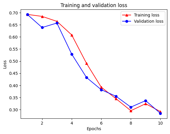
There are four entries: one for each monitored metric during training and validation. We can use these to plot the training and validation loss for comparison, as well as the training and validation accuracy:
acc = history_dict['accuracy']
val_acc = history_dict['val_accuracy']
loss = history_dict['loss']
val_loss = history_dict['val_loss']

epochs = range(1, len(acc) + 1)

# "-r^" is for solid red line with triangle markers.
plt.plot(epochs, loss, '-r^', label='Training loss')
# "-b0" is for solid blue line with circle markers.
plt.plot(epochs, val_loss, '-bo', label='Validation loss')
plt.title('Training and validation loss')
plt.xlabel('Epochs')
plt.ylabel('Loss')
plt.legend(loc='best')

plt.show()
plt.clf()   # clear figure

plt.plot(epochs, acc, '-r^', label='Training acc')
plt.plot(epochs, val_acc, '-bo', label='Validation acc')
plt.title('Training and validation accuracy')
plt.xlabel('Epochs')
plt.ylabel('Accuracy')
plt.legend(loc='best')

plt.show()
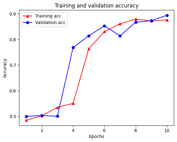
Notice the training loss decreases with each epoch and the training accuracy increases with each epoch. This is expected when using a gradient descent optimization—it should minimize the desired quantity on every iteration.
Graph regularization
We are now ready to try graph regularization using the base model that we built
above. We will use the GraphRegularization wrapper class provided by the
Neural Structured Learning framework to wrap the base (bi-LSTM) model to include
graph regularization. The rest of the steps for training and evaluating the
graph-regularized model are similar to that of the base model.
Create graph-regularized model
To assess the incremental benefit of graph regularization, we will create a new
base model instance. This is because model has already been trained for a few
iterations, and reusing this trained model to create a graph-regularized model
will not be a fair comparison for model.
# Build a new base LSTM model.
base_reg_model = make_bilstm_model()
# Wrap the base model with graph regularization.
graph_reg_config = nsl.configs.make_graph_reg_config(
    max_neighbors=HPARAMS.num_neighbors,
    multiplier=HPARAMS.graph_regularization_multiplier,
    distance_type=HPARAMS.distance_type,
    sum_over_axis=-1)
graph_reg_model = nsl.keras.GraphRegularization(base_reg_model,
                                                graph_reg_config)
graph_reg_model.compile(
    optimizer='adam',
    loss=tf.keras.losses.BinaryCrossentropy(from_logits=True),
    metrics=['accuracy'])
Train the model
graph_reg_history = graph_reg_model.fit(
    train_dataset,
    validation_data=validation_dataset,
    epochs=HPARAMS.train_epochs,
    verbose=1)
Epoch 1/10
WARNING:tensorflow:From /tmpfs/src/tf_docs_env/lib/python3.9/site-packages/tensorflow/python/autograph/pyct/static_analysis/liveness.py:83: Analyzer.lamba_check (from tensorflow.python.autograph.pyct.static_analysis.liveness) is deprecated and will be removed after 2023-09-23.
Instructions for updating:
Lambda fuctions will be no more assumed to be used in the statement where they are used, or at least in the same block. https://github.com/tensorflow/tensorflow/issues/56089
21/21 [==============================] - 27s 920ms/step - loss: 0.6938 - accuracy: 0.4858 - scaled_graph_loss: 3.3994e-05 - val_loss: 0.6928 - val_accuracy: 0.5024
Epoch 2/10
21/21 [==============================] - 17s 836ms/step - loss: 0.6921 - accuracy: 0.5085 - scaled_graph_loss: 2.2528e-05 - val_loss: 0.6916 - val_accuracy: 0.4987
Epoch 3/10
21/21 [==============================] - 18s 844ms/step - loss: 0.6806 - accuracy: 0.5088 - scaled_graph_loss: 0.0018 - val_loss: 0.6383 - val_accuracy: 0.6404
Epoch 4/10
21/21 [==============================] - 17s 837ms/step - loss: 0.6143 - accuracy: 0.6588 - scaled_graph_loss: 0.0292 - val_loss: 0.5993 - val_accuracy: 0.5436
Epoch 5/10
21/21 [==============================] - 17s 841ms/step - loss: 0.5748 - accuracy: 0.7015 - scaled_graph_loss: 0.0563 - val_loss: 0.4726 - val_accuracy: 0.8239
Epoch 6/10
21/21 [==============================] - 18s 847ms/step - loss: 0.5366 - accuracy: 0.8019 - scaled_graph_loss: 0.0681 - val_loss: 0.4708 - val_accuracy: 0.7508
Epoch 7/10
21/21 [==============================] - 18s 847ms/step - loss: 0.5330 - accuracy: 0.7992 - scaled_graph_loss: 0.0722 - val_loss: 0.4462 - val_accuracy: 0.8373
Epoch 8/10
21/21 [==============================] - 18s 848ms/step - loss: 0.5207 - accuracy: 0.8096 - scaled_graph_loss: 0.0755 - val_loss: 0.4772 - val_accuracy: 0.7738
Epoch 9/10
21/21 [==============================] - 18s 851ms/step - loss: 0.5139 - accuracy: 0.8319 - scaled_graph_loss: 0.0831 - val_loss: 0.4223 - val_accuracy: 0.8412
Epoch 10/10
21/21 [==============================] - 18s 851ms/step - loss: 0.4959 - accuracy: 0.8377 - scaled_graph_loss: 0.0813 - val_loss: 0.4332 - val_accuracy: 0.8199
Evaluate the model
graph_reg_results = graph_reg_model.evaluate(test_dataset, steps=HPARAMS.eval_steps)
print(graph_reg_results)
196/196 [==============================] - 15s 70ms/step - loss: 0.4728 - accuracy: 0.7732
[0.4728052020072937, 0.7731599807739258]
Create a graph of accuracy/loss over time
graph_reg_history_dict = graph_reg_history.history
graph_reg_history_dict.keys()
dict_keys(['loss', 'accuracy', 'scaled_graph_loss', 'val_loss', 'val_accuracy'])
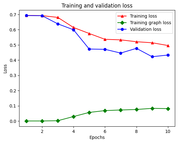
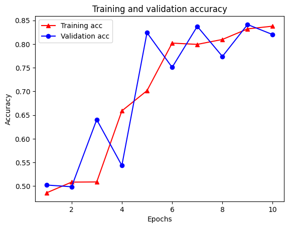
There are five entries in total in the dictionary: training loss, training accuracy, training graph loss, validation loss, and validation accuracy. We can plot them all together for comparison. Note that the graph loss is only computed during training.
acc = graph_reg_history_dict['accuracy']
val_acc = graph_reg_history_dict['val_accuracy']
loss = graph_reg_history_dict['loss']
graph_loss = graph_reg_history_dict['scaled_graph_loss']
val_loss = graph_reg_history_dict['val_loss']

epochs = range(1, len(acc) + 1)

plt.clf()   # clear figure

# "-r^" is for solid red line with triangle markers.
plt.plot(epochs, loss, '-r^', label='Training loss')
# "-gD" is for solid green line with diamond markers.
plt.plot(epochs, graph_loss, '-gD', label='Training graph loss')
# "-b0" is for solid blue line with circle markers.
plt.plot(epochs, val_loss, '-bo', label='Validation loss')
plt.title('Training and validation loss')
plt.xlabel('Epochs')
plt.ylabel('Loss')
plt.legend(loc='best')

plt.show()
plt.clf()   # clear figure

plt.plot(epochs, acc, '-r^', label='Training acc')
plt.plot(epochs, val_acc, '-bo', label='Validation acc')
plt.title('Training and validation accuracy')
plt.xlabel('Epochs')
plt.ylabel('Accuracy')
plt.legend(loc='best')

plt.show()
The power of semi-supervised learning
Semi-supervised learning and more specifically, graph regularization in the context of this tutorial, can be really powerful when the amount of training data is small. The lack of training data is compensated by leveraging similarity among the training samples, which is not possible in traditional supervised learning.
We define supervision ratio as the ratio of training samples to the total number of samples which includes training, validation, and test samples. In this notebook, we have used a supervision ratio of 0.05 (i.e, 5% of the labeled data) for training both the base model as well as the graph-regularized model. We illustrate the impact of the supervision ratio on model accuracy in the cell below.
# Accuracy values for both the Bi-LSTM model and the feed forward NN model have
# been precomputed for the following supervision ratios.

supervision_ratios = [0.3, 0.15, 0.05, 0.03, 0.02, 0.01, 0.005]

model_tags = ['Bi-LSTM model', 'Feed Forward NN model']
base_model_accs = [[84, 84, 83, 80, 65, 52, 50], [87, 86, 76, 74, 67, 52, 51]]
graph_reg_model_accs = [[84, 84, 83, 83, 65, 63, 50],
                        [87, 86, 80, 75, 67, 52, 50]]

plt.clf()  # clear figure

fig, axes = plt.subplots(1, 2)
fig.set_size_inches((12, 5))

for ax, model_tag, base_model_acc, graph_reg_model_acc in zip(
    axes, model_tags, base_model_accs, graph_reg_model_accs):

  # "-r^" is for solid red line with triangle markers.
  ax.plot(base_model_acc, '-r^', label='Base model')
  # "-gD" is for solid green line with diamond markers.
  ax.plot(graph_reg_model_acc, '-gD', label='Graph-regularized model')
  ax.set_title(model_tag)
  ax.set_xlabel('Supervision ratio')
  ax.set_ylabel('Accuracy(%)')
  ax.set_ylim((25, 100))
  ax.set_xticks(range(len(supervision_ratios)))
  ax.set_xticklabels(supervision_ratios)
  ax.legend(loc='best')

plt.show()
<Figure size 640x480 with 0 Axes>
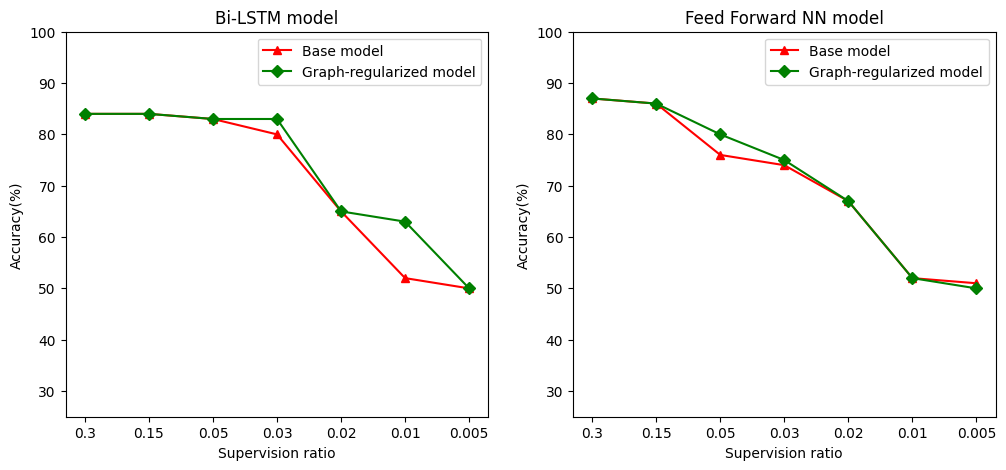
It can be observed that as the superivision ratio decreases, model accuracy also decreases. This is true for both the base model and for the graph-regularized model, regardless of the model architecture used. However, notice that the graph-regularized model performs better than the base model for both the architectures. In particular, for the Bi-LSTM model, when the supervision ratio is 0.01, the accuracy of the graph-regularized model is ~20% higher than that of the base model. This is primarily because of semi-supervised learning for the graph-regularized model, where structural similarity among training samples is used in addition to the training samples themselves.
Conclusion
We have demonstrated the use of graph regularization using the Neural Structured Learning (NSL) framework even when the input does not contain an explicit graph. We considered the task of sentiment classification of IMDB movie reviews for which we synthesized a similarity graph based on review embeddings. We encourage users to experiment further by varying hyperparameters, the amount of supervision, and by using different model architectures.