
|
|
|
 View source on GitHub View source on GitHub
|
|
|
This tutorial demonstrates how to fine-tune a Bidirectional Encoder Representations from Transformers (BERT) (Devlin et al., 2018) model using TensorFlow Model Garden.
You can also find the pre-trained BERT model used in this tutorial on TensorFlow Hub (TF Hub). For concrete examples of how to use the models from TF Hub, refer to the Solve Glue tasks using BERT tutorial. If you're just trying to fine-tune a model, the TF Hub tutorial is a good starting point.
On the other hand, if you're interested in deeper customization, follow this tutorial. It shows how to do a lot of things manually, so you can learn how you can customize the workflow from data preprocessing to training, exporting and saving the model.
Setup
Install pip packages
Start by installing the TensorFlow Text and Model Garden pip packages.
tf-models-officialis the TensorFlow Model Garden package. Note that it may not include the latest changes in thetensorflow_modelsGitHub repo. To include the latest changes, you may installtf-models-nightly, which is the nightly Model Garden package created daily automatically.- pip will install all models and dependencies automatically.
pip install -q opencv-pythonpip install -q -U "tensorflow-text==2.11.*"pip install -q tf-models-officialImport libraries
import os

import numpy as np
import matplotlib.pyplot as plt

import tensorflow as tf
import tensorflow_models as tfm
import tensorflow_hub as hub
import tensorflow_datasets as tfds
tfds.disable_progress_bar()
2024-02-07 12:13:37.890233: E external/local_xla/xla/stream_executor/cuda/cuda_dnn.cc:9261] Unable to register cuDNN factory: Attempting to register factory for plugin cuDNN when one has already been registered
2024-02-07 12:13:37.890282: E external/local_xla/xla/stream_executor/cuda/cuda_fft.cc:607] Unable to register cuFFT factory: Attempting to register factory for plugin cuFFT when one has already been registered
2024-02-07 12:13:37.891884: E external/local_xla/xla/stream_executor/cuda/cuda_blas.cc:1515] Unable to register cuBLAS factory: Attempting to register factory for plugin cuBLAS when one has already been registered
Resources
The following directory contains the BERT model's configuration, vocabulary, and a pre-trained checkpoint used in this tutorial:
gs_folder_bert = "gs://cloud-tpu-checkpoints/bert/v3/uncased_L-12_H-768_A-12"
tf.io.gfile.listdir(gs_folder_bert)
['bert_config.json',
 'bert_model.ckpt.data-00000-of-00001',
 'bert_model.ckpt.index',
 'vocab.txt']
Load and preprocess the dataset
This example uses the GLUE (General Language Understanding Evaluation) MRPC (Microsoft Research Paraphrase Corpus) dataset from TensorFlow Datasets (TFDS).
This dataset is not set up such that it can be directly fed into the BERT model. The following section handles the necessary preprocessing.
Get the dataset from TensorFlow Datasets
The GLUE MRPC (Dolan and Brockett, 2005) dataset is a corpus of sentence pairs automatically extracted from online news sources, with human annotations for whether the sentences in the pair are semantically equivalent. It has the following attributes:
- Number of labels: 2
- Size of training dataset: 3668
- Size of evaluation dataset: 408
- Maximum sequence length of training and evaluation dataset: 128
Begin by loading the MRPC dataset from TFDS:
batch_size=32
glue, info = tfds.load('glue/mrpc',
                       with_info=True,
                       batch_size=32)
glue
{'train': <_PrefetchDataset element_spec={'idx': TensorSpec(shape=(None,), dtype=tf.int32, name=None), 'label': TensorSpec(shape=(None,), dtype=tf.int64, name=None), 'sentence1': TensorSpec(shape=(None,), dtype=tf.string, name=None), 'sentence2': TensorSpec(shape=(None,), dtype=tf.string, name=None)}>,
 'validation': <_PrefetchDataset element_spec={'idx': TensorSpec(shape=(None,), dtype=tf.int32, name=None), 'label': TensorSpec(shape=(None,), dtype=tf.int64, name=None), 'sentence1': TensorSpec(shape=(None,), dtype=tf.string, name=None), 'sentence2': TensorSpec(shape=(None,), dtype=tf.string, name=None)}>,
 'test': <_PrefetchDataset element_spec={'idx': TensorSpec(shape=(None,), dtype=tf.int32, name=None), 'label': TensorSpec(shape=(None,), dtype=tf.int64, name=None), 'sentence1': TensorSpec(shape=(None,), dtype=tf.string, name=None), 'sentence2': TensorSpec(shape=(None,), dtype=tf.string, name=None)}>}
The info object describes the dataset and its features:
info.features
FeaturesDict({
    'idx': int32,
    'label': ClassLabel(shape=(), dtype=int64, num_classes=2),
    'sentence1': Text(shape=(), dtype=string),
    'sentence2': Text(shape=(), dtype=string),
})
The two classes are:
info.features['label'].names
['not_equivalent', 'equivalent']
Here is one example from the training set:
example_batch = next(iter(glue['train']))

for key, value in example_batch.items():
  print(f"{key:9s}: {value[0].numpy()}")
idx      : 1680
label    : 0
sentence1: b'The identical rovers will act as robotic geologists , searching for evidence of past water .'
sentence2: b'The rovers act as robotic geologists , moving on six wheels .'
2024-02-07 12:13:45.153482: W tensorflow/core/kernels/data/cache_dataset_ops.cc:858] The calling iterator did not fully read the dataset being cached. In order to avoid unexpected truncation of the dataset, the partially cached contents of the dataset  will be discarded. This can happen if you have an input pipeline similar to `dataset.cache().take(k).repeat()`. You should use `dataset.take(k).cache().repeat()` instead.
Preprocess the data
The keys "sentence1" and "sentence2" in the GLUE MRPC dataset contain two input sentences for each example.
Because the BERT model from the Model Garden doesn't take raw text as input, two things need to happen first:
- The text needs to be tokenized (split into word pieces) and converted to indices.
- Then, the indices need to be packed into the format that the model expects.
The BERT tokenizer
To fine tune a pre-trained language model from the Model Garden, such as BERT, you need to make sure that you're using exactly the same tokenization, vocabulary, and index mapping as used during training.
The following code rebuilds the tokenizer that was used by the base model using the Model Garden's tfm.nlp.layers.FastWordpieceBertTokenizer layer:
tokenizer = tfm.nlp.layers.FastWordpieceBertTokenizer(
    vocab_file=os.path.join(gs_folder_bert, "vocab.txt"),
    lower_case=True)
Let's tokenize a test sentence:
tokens = tokenizer(tf.constant(["Hello TensorFlow!"]))
tokens
<tf.RaggedTensor [[[7592], [23435, 12314], [999]]]>
Learn more about the tokenization process in the Subword tokenization and Tokenizing with TensorFlow Text guides.
Pack the inputs
TensorFlow Model Garden's BERT model doesn't just take the tokenized strings as input. It also expects these to be packed into a particular format. tfm.nlp.layers.BertPackInputs layer can handle the conversion from a list of tokenized sentences to the input format expected by the Model Garden's BERT model.
tfm.nlp.layers.BertPackInputs packs the two input sentences (per example in the MRCP dataset) concatenated together. This input is expected to start with a [CLS] "This is a classification problem" token, and each sentence should end with a [SEP] "Separator" token.
Therefore, the tfm.nlp.layers.BertPackInputs layer's constructor takes the tokenizer's special tokens as an argument. It also needs to know the indices of the tokenizer's special tokens.
special = tokenizer.get_special_tokens_dict()
special
{'vocab_size': 30522,
 'start_of_sequence_id': 101,
 'end_of_segment_id': 102,
 'padding_id': 0,
 'mask_id': 103}
max_seq_length = 128

packer = tfm.nlp.layers.BertPackInputs(
    seq_length=max_seq_length,
    special_tokens_dict = tokenizer.get_special_tokens_dict())
The packer takes a list of tokenized sentences as input. For example:
sentences1 = ["hello tensorflow"]
tok1 = tokenizer(sentences1)
tok1
<tf.RaggedTensor [[[7592], [23435, 12314]]]>
sentences2 = ["goodbye tensorflow"]
tok2 = tokenizer(sentences2)
tok2
<tf.RaggedTensor [[[9119], [23435, 12314]]]>
Then, it returns a dictionary containing three outputs:
input_word_ids: The tokenized sentences packed together.input_mask: The mask indicating which locations are valid in the other outputs.input_type_ids: Indicating which sentence each token belongs to.
packed = packer([tok1, tok2])

for key, tensor in packed.items():
  print(f"{key:15s}: {tensor[:, :12]}")
input_word_ids : [[  101  7592 23435 12314   102  9119 23435 12314   102     0     0     0]]
input_mask     : [[1 1 1 1 1 1 1 1 1 0 0 0]]
input_type_ids : [[0 0 0 0 0 1 1 1 1 0 0 0]]
Put it all together
Combine these two parts into a keras.layers.Layer that can be attached to your model:
class BertInputProcessor(tf.keras.layers.Layer):
  def __init__(self, tokenizer, packer):
    super().__init__()
    self.tokenizer = tokenizer
    self.packer = packer

  def call(self, inputs):
    tok1 = self.tokenizer(inputs['sentence1'])
    tok2 = self.tokenizer(inputs['sentence2'])

    packed = self.packer([tok1, tok2])

    if 'label' in inputs:
      return packed, inputs['label']
    else:
      return packed
But for now just apply it to the dataset using Dataset.map, since the dataset you loaded from TFDS is a tf.data.Dataset object:
bert_inputs_processor = BertInputProcessor(tokenizer, packer)
glue_train = glue['train'].map(bert_inputs_processor).prefetch(1)
Here is an example batch from the processed dataset:
example_inputs, example_labels = next(iter(glue_train))
2024-02-07 12:13:49.744645: W tensorflow/core/kernels/data/cache_dataset_ops.cc:858] The calling iterator did not fully read the dataset being cached. In order to avoid unexpected truncation of the dataset, the partially cached contents of the dataset will be discarded. This can happen if you have an input pipeline similar to `dataset.cache().take(k).repeat()`. You should use `dataset.take(k).cache().repeat()` instead.
example_inputs
{'input_word_ids': <tf.Tensor: shape=(32, 128), dtype=int32, numpy=
 array([[ 101, 1996, 7235, ...,    0,    0,    0],
        [ 101, 2625, 2084, ...,    0,    0,    0],
        [ 101, 6804, 1011, ...,    0,    0,    0],
        ...,
        [ 101, 2021, 2049, ...,    0,    0,    0],
        [ 101, 2274, 2062, ...,    0,    0,    0],
        [ 101, 2043, 1037, ...,    0,    0,    0]], dtype=int32)>,
 'input_mask': <tf.Tensor: shape=(32, 128), dtype=int32, numpy=
 array([[1, 1, 1, ..., 0, 0, 0],
        [1, 1, 1, ..., 0, 0, 0],
        [1, 1, 1, ..., 0, 0, 0],
        ...,
        [1, 1, 1, ..., 0, 0, 0],
        [1, 1, 1, ..., 0, 0, 0],
        [1, 1, 1, ..., 0, 0, 0]], dtype=int32)>,
 'input_type_ids': <tf.Tensor: shape=(32, 128), dtype=int32, numpy=
 array([[0, 0, 0, ..., 0, 0, 0],
        [0, 0, 0, ..., 0, 0, 0],
        [0, 0, 0, ..., 0, 0, 0],
        ...,
        [0, 0, 0, ..., 0, 0, 0],
        [0, 0, 0, ..., 0, 0, 0],
        [0, 0, 0, ..., 0, 0, 0]], dtype=int32)>}
example_labels
<tf.Tensor: shape=(32,), dtype=int64, numpy=
array([0, 0, 1, 1, 0, 0, 1, 1, 1, 1, 1, 1, 0, 1, 1, 0, 1, 1, 1, 0, 1, 1,
       1, 1, 1, 1, 1, 0, 0, 1, 0, 1])>
for key, value in example_inputs.items():
  print(f'{key:15s} shape: {value.shape}')

print(f'{"labels":15s} shape: {example_labels.shape}')
input_word_ids  shape: (32, 128)
input_mask      shape: (32, 128)
input_type_ids  shape: (32, 128)
labels          shape: (32,)
The input_word_ids contain the token IDs:
plt.pcolormesh(example_inputs['input_word_ids'])
<matplotlib.collections.QuadMesh at 0x7f0f10480250>
The mask allows the model to cleanly differentiate between the content and the padding. The mask has the same shape as the input_word_ids, and contains a 1 anywhere the input_word_ids is not padding.
plt.pcolormesh(example_inputs['input_mask'])
<matplotlib.collections.QuadMesh at 0x7f0f500ce670>
The "input type" also has the same shape, but inside the non-padded region, contains a 0 or a 1 indicating which sentence the token is a part of.
plt.pcolormesh(example_inputs['input_type_ids'])
<matplotlib.collections.QuadMesh at 0x7f0f201d4700>
Apply the same preprocessing to the validation and test subsets of the GLUE MRPC dataset:
glue_validation = glue['validation'].map(bert_inputs_processor).prefetch(1)
glue_test = glue['test'].map(bert_inputs_processor).prefetch(1)
Build, train and export the model
Now that you have formatted the data as expected, you can start working on building and training the model.
Build the model
The first step is to download the configuration file—config_dict—for the pre-trained BERT model:
import json

bert_config_file = os.path.join(gs_folder_bert, "bert_config.json")
config_dict = json.loads(tf.io.gfile.GFile(bert_config_file).read())
config_dict
{'attention_probs_dropout_prob': 0.1,
 'hidden_act': 'gelu',
 'hidden_dropout_prob': 0.1,
 'hidden_size': 768,
 'initializer_range': 0.02,
 'intermediate_size': 3072,
 'max_position_embeddings': 512,
 'num_attention_heads': 12,
 'num_hidden_layers': 12,
 'type_vocab_size': 2,
 'vocab_size': 30522}
encoder_config = tfm.nlp.encoders.EncoderConfig({
    'type':'bert',
    'bert': config_dict
})
bert_encoder = tfm.nlp.encoders.build_encoder(encoder_config)
bert_encoder
<official.nlp.modeling.networks.bert_encoder.BertEncoder at 0x7f0f103d16d0>
The configuration file defines the core BERT model from the Model Garden, which is a Keras model that predicts the outputs of num_classes from the inputs with maximum sequence length max_seq_length.
bert_classifier = tfm.nlp.models.BertClassifier(network=bert_encoder, num_classes=2)
Run it on a test batch of data 10 examples from the training set. The output is the logits for the two classes:
bert_classifier(
    example_inputs, training=True).numpy()[:10]
array([[ 0.08335936,  1.1473498 ],
       [ 1.3190541 ,  1.3408866 ],
       [ 0.19908446,  0.7913456 ],
       [ 0.48186374,  1.2114024 ],
       [ 0.9708527 ,  0.7837988 ],
       [ 0.25541633,  0.76591694],
       [ 1.3683597 ,  1.0795705 ],
       [ 0.11288509,  1.1301354 ],
       [-0.02536219,  0.4678782 ],
       [ 0.9831672 ,  0.538211  ]], dtype=float32)
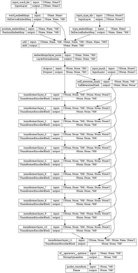
The TransformerEncoder in the center of the classifier above is the bert_encoder.
If you inspect the encoder, notice the stack of Transformer layers connected to those same three inputs:
tf.keras.utils.plot_model(bert_encoder, show_shapes=True, dpi=48)
Restore the encoder weights
When built, the encoder is randomly initialized. Restore the encoder's weights from the checkpoint:
checkpoint = tf.train.Checkpoint(encoder=bert_encoder)
checkpoint.read(
    os.path.join(gs_folder_bert, 'bert_model.ckpt')).assert_consumed()
<tensorflow.python.checkpoint.checkpoint.CheckpointLoadStatus at 0x7f105f713cd0>
Set up the optimizer
BERT typically uses the Adam optimizer with weight decay—AdamW (tf.keras.optimizers.experimental.AdamW).
It also employs a learning rate schedule that first warms up from 0 and then decays to 0:
# Set up epochs and steps
epochs = 5
batch_size = 32
eval_batch_size = 32

train_data_size = info.splits['train'].num_examples
steps_per_epoch = int(train_data_size / batch_size)
num_train_steps = steps_per_epoch * epochs
warmup_steps = int(0.1 * num_train_steps)
initial_learning_rate=2e-5
Linear decay from initial_learning_rate to zero over num_train_steps.
linear_decay = tf.keras.optimizers.schedules.PolynomialDecay(
    initial_learning_rate=initial_learning_rate,
    end_learning_rate=0,
    decay_steps=num_train_steps)
Warmup to that value over warmup_steps:
warmup_schedule = tfm.optimization.lr_schedule.LinearWarmup(
    warmup_learning_rate = 0,
    after_warmup_lr_sched = linear_decay,
    warmup_steps = warmup_steps
)
The overall schedule looks like this:
x = tf.linspace(0, num_train_steps, 1001)
y = [warmup_schedule(xi) for xi in x]
plt.plot(x,y)
plt.xlabel('Train step')
plt.ylabel('Learning rate')
Text(0, 0.5, 'Learning rate')
Use tf.keras.optimizers.experimental.AdamW to instantiate the optimizer with that schedule:
optimizer = tf.keras.optimizers.experimental.Adam(
    learning_rate = warmup_schedule)
Train the model
Set the metric as accuracy and the loss as sparse categorical cross-entropy. Then, compile and train the BERT classifier:
metrics = [tf.keras.metrics.SparseCategoricalAccuracy('accuracy', dtype=tf.float32)]
loss = tf.keras.losses.SparseCategoricalCrossentropy(from_logits=True)

bert_classifier.compile(
    optimizer=optimizer,
    loss=loss,
    metrics=metrics)
bert_classifier.evaluate(glue_validation)
13/13 [==============================] - 6s 255ms/step - loss: 1.1962 - accuracy: 0.3162
[1.1962156295776367, 0.31617647409439087]
bert_classifier.fit(
      glue_train,
      validation_data=(glue_validation),
      batch_size=32,
      epochs=epochs)
Epoch 1/5
WARNING: All log messages before absl::InitializeLog() is called are written to STDERR
I0000 00:00:1707308071.926522   10692 device_compiler.h:186] Compiled cluster using XLA!  This line is logged at most once for the lifetime of the process.
115/115 [==============================] - 131s 858ms/step - loss: 0.7210 - accuracy: 0.6191 - val_loss: 0.5249 - val_accuracy: 0.7426
Epoch 2/5
115/115 [==============================] - 101s 875ms/step - loss: 0.4744 - accuracy: 0.7751 - val_loss: 0.4766 - val_accuracy: 0.8064
Epoch 3/5
115/115 [==============================] - 101s 877ms/step - loss: 0.3204 - accuracy: 0.8642 - val_loss: 0.4100 - val_accuracy: 0.8333
Epoch 4/5
115/115 [==============================] - 101s 878ms/step - loss: 0.2006 - accuracy: 0.9278 - val_loss: 0.4783 - val_accuracy: 0.8358
Epoch 5/5
115/115 [==============================] - 101s 879ms/step - loss: 0.1323 - accuracy: 0.9577 - val_loss: 0.4668 - val_accuracy: 0.8382
<keras.src.callbacks.History at 0x7f105f702250>
Now run the fine-tuned model on a custom example to see that it works.
Start by encoding some sentence pairs:
my_examples = {
        'sentence1':[
            'The rain in Spain falls mainly on the plain.',
            'Look I fine tuned BERT.'],
        'sentence2':[
            'It mostly rains on the flat lands of Spain.',
            'Is it working? This does not match.']
    }
The model should report class 1 "match" for the first example and class 0 "no-match" for the second:
ex_packed = bert_inputs_processor(my_examples)
my_logits = bert_classifier(ex_packed, training=False)

result_cls_ids = tf.argmax(my_logits)
result_cls_ids
<tf.Tensor: shape=(2,), dtype=int64, numpy=array([1, 0])>
tf.gather(tf.constant(info.features['label'].names), result_cls_ids)
<tf.Tensor: shape=(2,), dtype=string, numpy=array([b'equivalent', b'not_equivalent'], dtype=object)>
Export the model
Often the goal of training a model is to use it for something outside of the Python process that created it. You can do this by exporting the model using tf.saved_model. (Learn more in the Using the SavedModel format guide and the Save and load a model using a distribution strategy tutorial.)
First, build a wrapper class to export the model. This wrapper does two things:
- First, it packages
bert_inputs_processorandbert_classifiertogether into a singletf.Module, so you can export all the functionalities. - Second, it defines a
tf.functionthat implements the end-to-end execution of the model.
Setting the input_signature argument of tf.function lets you define a fixed signature for the tf.function. This can be less surprising than the default automatic retracing behavior.
class ExportModel(tf.Module):
  def __init__(self, input_processor, classifier):
    self.input_processor = input_processor
    self.classifier = classifier

  @tf.function(input_signature=[{
      'sentence1': tf.TensorSpec(shape=[None], dtype=tf.string),
      'sentence2': tf.TensorSpec(shape=[None], dtype=tf.string)}])
  def __call__(self, inputs):
    packed = self.input_processor(inputs)
    logits =  self.classifier(packed, training=False)
    result_cls_ids = tf.argmax(logits)
    return {
        'logits': logits,
        'class_id': result_cls_ids,
        'class': tf.gather(
            tf.constant(info.features['label'].names),
            result_cls_ids)
    }
Create an instance of this exported model and save it:
export_model = ExportModel(bert_inputs_processor, bert_classifier)
import tempfile
export_dir=tempfile.mkdtemp(suffix='_saved_model')
tf.saved_model.save(export_model, export_dir=export_dir,
                    signatures={'serving_default': export_model.__call__})
INFO:tensorflow:Assets written to: /tmpfs/tmp/tmpxj846i17_saved_model/assets
INFO:tensorflow:Assets written to: /tmpfs/tmp/tmpxj846i17_saved_model/assets
Reload the model and compare the results to the original:
original_logits = export_model(my_examples)['logits']
reloaded = tf.saved_model.load(export_dir)
reloaded_logits = reloaded(my_examples)['logits']
# The results are identical:
print(original_logits.numpy())
print()
print(reloaded_logits.numpy())
[[-2.7769644  2.3126464]
 [ 1.4339567 -1.1664971]]

[[-2.7769644  2.3126464]
 [ 1.4339567 -1.1664971]]
print(np.mean(abs(original_logits - reloaded_logits)))
0.0
Congratulations! You've used tensorflow_models to build a BERT-classifier, train it, and export it for later use.
Optional: BERT on TF Hub
You can get the BERT model off the shelf from TF Hub. There are many versions available along with their input preprocessors.
This example uses a small version of BERT from TF Hub that was pre-trained using the English Wikipedia and BooksCorpus datasets, similar to the original implementation (Turc et al., 2019).
Start by importing TF Hub:
import tensorflow_hub as hub
Select the input preprocessor and the model from TF Hub and wrap them as hub.KerasLayer layers:
# Always make sure you use the right preprocessor.
hub_preprocessor = hub.KerasLayer(
    "https://tfhub.dev/tensorflow/bert_en_uncased_preprocess/3")

# This is a really small BERT.
hub_encoder = hub.KerasLayer(f"https://tfhub.dev/tensorflow/small_bert/bert_en_uncased_L-2_H-128_A-2/2",
                             trainable=True)

print(f"The Hub encoder has {len(hub_encoder.trainable_variables)} trainable variables")
The Hub encoder has 39 trainable variables
Test run the preprocessor on a batch of data:
hub_inputs = hub_preprocessor(['Hello TensorFlow!'])
{key: value[0, :10].numpy() for key, value in hub_inputs.items()}
{'input_type_ids': array([0, 0, 0, 0, 0, 0, 0, 0, 0, 0], dtype=int32),
 'input_word_ids': array([  101,  7592, 23435, 12314,   999,   102,     0,     0,     0,
            0], dtype=int32),
 'input_mask': array([1, 1, 1, 1, 1, 1, 0, 0, 0, 0], dtype=int32)}
result = hub_encoder(
    inputs=hub_inputs,
    training=False,
)

print("Pooled output shape:", result['pooled_output'].shape)
print("Sequence output shape:", result['sequence_output'].shape)
Pooled output shape: (1, 128)
Sequence output shape: (1, 128, 128)
At this point, it would be simple to add a classification head yourself.
The Model Garden tfm.nlp.models.BertClassifier class can also build a classifier onto the TF Hub encoder:
hub_classifier = tfm.nlp.models.BertClassifier(
    bert_encoder,
    num_classes=2,
    dropout_rate=0.1,
    initializer=tf.keras.initializers.TruncatedNormal(
        stddev=0.02))
The one downside to loading this model from TF Hub is that the structure of internal Keras layers is not restored. This makes it more difficult to inspect or modify the model.
The BERT encoder model—hub_classifier—is now a single layer.
For concrete examples of this approach, refer to Solve Glue tasks using the BERT.
Optional: Optimizer configs
The tensorflow_models package defines serializable config classes that describe how to build the live objects. Earlier in this tutorial, you built the optimizer manually.
The configuration below describes an (almost) identical optimizer built by the optimizer_factory.OptimizerFactory:
optimization_config = tfm.optimization.OptimizationConfig(
    optimizer=tfm.optimization.OptimizerConfig(
        type = "adam"),
    learning_rate = tfm.optimization.LrConfig(
        type='polynomial',
        polynomial=tfm.optimization.PolynomialLrConfig(
            initial_learning_rate=2e-5,
            end_learning_rate=0.0,
            decay_steps=num_train_steps)),
    warmup = tfm.optimization.WarmupConfig(
        type='linear',
        linear=tfm.optimization.LinearWarmupConfig(warmup_steps=warmup_steps)
    ))


fac = tfm.optimization.optimizer_factory.OptimizerFactory(optimization_config)
lr = fac.build_learning_rate()
optimizer = fac.build_optimizer(lr=lr)
x = tf.linspace(0, num_train_steps, 1001).numpy()
y = [lr(xi) for xi in x]
plt.plot(x,y)
plt.xlabel('Train step')
plt.ylabel('Learning rate')
Text(0, 0.5, 'Learning rate')
The advantage of using config objects is that they don't contain any complicated TensorFlow objects, and can be easily serialized to JSON, and rebuilt. Here's the JSON for the above tfm.optimization.OptimizationConfig:
optimization_config = optimization_config.as_dict()
optimization_config
{'optimizer': {'type': 'adam',
  'adam': {'clipnorm': None,
   'clipvalue': None,
   'global_clipnorm': None,
   'name': 'Adam',
   'beta_1': 0.9,
   'beta_2': 0.999,
   'epsilon': 1e-07,
   'amsgrad': False} },
 'ema': None,
 'learning_rate': {'type': 'polynomial',
  'polynomial': {'name': 'PolynomialDecay',
   'initial_learning_rate': 2e-05,
   'decay_steps': 570,
   'end_learning_rate': 0.0,
   'power': 1.0,
   'cycle': False,
   'offset': 0} },
 'warmup': {'type': 'linear',
  'linear': {'name': 'linear', 'warmup_learning_rate': 0, 'warmup_steps': 57} } }
The tfm.optimization.optimizer_factory.OptimizerFactory can just as easily build the optimizer from the JSON dictionary:
fac = tfm.optimization.optimizer_factory.OptimizerFactory(
    tfm.optimization.OptimizationConfig(optimization_config))
lr = fac.build_learning_rate()
optimizer = fac.build_optimizer(lr=lr)