
|
|
|
 View source on GitHub View source on GitHub
|
|
Overview
Using the TensorFlow Image Summary API, you can easily log tensors and arbitrary images and view them in TensorBoard. This can be extremely helpful to sample and examine your input data, or to visualize layer weights and generated tensors. You can also log diagnostic data as images that can be helpful in the course of your model development.
In this tutorial, you will learn how to use the Image Summary API to visualize tensors as images. You will also learn how to take an arbitrary image, convert it to a tensor, and visualize it in TensorBoard. You will work through a simple but real example that uses Image Summaries to help you understand how your model is performing.
Setup
try:
  # %tensorflow_version only exists in Colab.
  %tensorflow_version 2.x
except Exception:
  pass

# Load the TensorBoard notebook extension.
%load_ext tensorboard
TensorFlow 2.x selected.
from datetime import datetime
import io
import itertools
from packaging import version

import tensorflow as tf
from tensorflow import keras

import matplotlib.pyplot as plt
import numpy as np
import sklearn.metrics

print("TensorFlow version: ", tf.__version__)
assert version.parse(tf.__version__).release[0] >= 2, \
    "This notebook requires TensorFlow 2.0 or above."
TensorFlow version: 2.2
Download the Fashion-MNIST dataset
You're going to construct a simple neural network to classify images in the the Fashion-MNIST dataset. This dataset consist of 70,000 28x28 grayscale images of fashion products from 10 categories, with 7,000 images per category.
First, download the data:
# Download the data. The data is already divided into train and test.
# The labels are integers representing classes.
fashion_mnist = keras.datasets.fashion_mnist
(train_images, train_labels), (test_images, test_labels) = \
    fashion_mnist.load_data()

# Names of the integer classes, i.e., 0 -> T-short/top, 1 -> Trouser, etc.
class_names = ['T-shirt/top', 'Trouser', 'Pullover', 'Dress', 'Coat',
    'Sandal', 'Shirt', 'Sneaker', 'Bag', 'Ankle boot']
Downloading data from https://storage.googleapis.com/tensorflow/tf-keras-datasets/train-labels-idx1-ubyte.gz
32768/29515 [=================================] - 0s 0us/step
Downloading data from https://storage.googleapis.com/tensorflow/tf-keras-datasets/train-images-idx3-ubyte.gz
26427392/26421880 [==============================] - 0s 0us/step
Downloading data from https://storage.googleapis.com/tensorflow/tf-keras-datasets/t10k-labels-idx1-ubyte.gz
8192/5148 [===============================================] - 0s 0us/step
Downloading data from https://storage.googleapis.com/tensorflow/tf-keras-datasets/t10k-images-idx3-ubyte.gz
4423680/4422102 [==============================] - 0s 0us/step
Visualizing a single image
To understand how the Image Summary API works, you're now going to simply log the first training image in your training set in TensorBoard.
Before you do that, examine the shape of your training data:
print("Shape: ", train_images[0].shape)
print("Label: ", train_labels[0], "->", class_names[train_labels[0]])
Shape:  (28, 28)
Label:  9 -> Ankle boot
Notice that the shape of each image in the data set is a rank-2 tensor of shape (28, 28), representing the height and the width.
However, tf.summary.image() expects a rank-4 tensor containing (batch_size, height, width, channels). Therefore, the tensors need to be reshaped.
You're logging only one image, so batch_size is 1. The images are grayscale, so set channels to 1.
# Reshape the image for the Summary API.
img = np.reshape(train_images[0], (-1, 28, 28, 1))
You're now ready to log this image and view it in TensorBoard.
# Clear out any prior log data.
!rm -rf logs

# Sets up a timestamped log directory.
logdir = "logs/train_data/" + datetime.now().strftime("%Y%m%d-%H%M%S")
# Creates a file writer for the log directory.
file_writer = tf.summary.create_file_writer(logdir)

# Using the file writer, log the reshaped image.
with file_writer.as_default():
  tf.summary.image("Training data", img, step=0)
Now, use TensorBoard to examine the image. Wait a few seconds for the UI to spin up.
%tensorboard --logdir logs/train_data

The "Time Series" dashboard displays the image you just logged. It's an "ankle boot".
The image is scaled to a default size for easier viewing. If you want to view the unscaled original image, check "Show actual image size" at the bottom of the "Settings" panel on the right.
Play with the brightness and contrast sliders to see how they affect the image pixels.
Visualizing multiple images
Logging one tensor is great, but what if you wanted to log multiple training examples?
Simply specify the number of images you want to log when passing data to tf.summary.image().
with file_writer.as_default():
  # Don't forget to reshape.
  images = np.reshape(train_images[0:25], (-1, 28, 28, 1))
  tf.summary.image("25 training data examples", images, max_outputs=25, step=0)

%tensorboard --logdir logs/train_data

Logging arbitrary image data
What if you want to visualize an image that's not a tensor, such as an image generated by matplotlib?
You need some boilerplate code to convert the plot to a tensor, but after that, you're good to go.
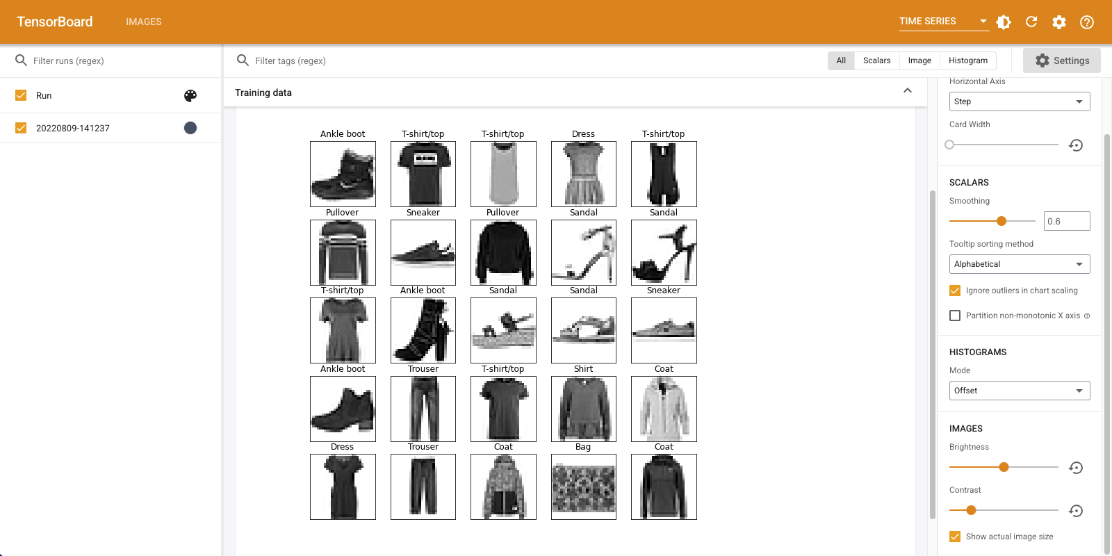
In the code below, you'll log the first 25 images as a nice grid using matplotlib's subplot() function. You'll then view the grid in TensorBoard:
# Clear out prior logging data.
!rm -rf logs/plots

logdir = "logs/plots/" + datetime.now().strftime("%Y%m%d-%H%M%S")
file_writer = tf.summary.create_file_writer(logdir)

def plot_to_image(figure):
  """Converts the matplotlib plot specified by 'figure' to a PNG image and
  returns it. The supplied figure is closed and inaccessible after this call."""
  # Save the plot to a PNG in memory.
  buf = io.BytesIO()
  plt.savefig(buf, format='png')
  # Closing the figure prevents it from being displayed directly inside
  # the notebook.
  plt.close(figure)
  buf.seek(0)
  # Convert PNG buffer to TF image
  image = tf.image.decode_png(buf.getvalue(), channels=4)
  # Add the batch dimension
  image = tf.expand_dims(image, 0)
  return image

def image_grid():
  """Return a 5x5 grid of the MNIST images as a matplotlib figure."""
  # Create a figure to contain the plot.
  figure = plt.figure(figsize=(10,10))
  for i in range(25):
    # Start next subplot.
    plt.subplot(5, 5, i + 1, title=class_names[train_labels[i]])
    plt.xticks([])
    plt.yticks([])
    plt.grid(False)
    plt.imshow(train_images[i], cmap=plt.cm.binary)

  return figure

# Prepare the plot
figure = image_grid()
# Convert to image and log
with file_writer.as_default():
  tf.summary.image("Training data", plot_to_image(figure), step=0)

%tensorboard --logdir logs/plots
Building an image classifier
Now put this all together with a real example. After all, you're here to do machine learning and not plot pretty pictures!
You're going to use image summaries to understand how well your model is doing while training a simple classifier for the Fashion-MNIST dataset.
First, create a very simple model and compile it, setting up the optimizer and loss function. The compile step also specifies that you want to log the accuracy of the classifier along the way.
model = keras.models.Sequential([
    keras.layers.Flatten(input_shape=(28, 28)),
    keras.layers.Dense(32, activation='relu'),
    keras.layers.Dense(10, activation='softmax')
])

model.compile(
    optimizer='adam',
    loss='sparse_categorical_crossentropy',
    metrics=['accuracy']
)
When training a classifier, it's useful to see the confusion matrix. The confusion matrix gives you detailed knowledge of how your classifier is performing on test data.
Define a function that calculates the confusion matrix. You'll use a convenient Scikit-learn function to do this, and then plot it using matplotlib.
def plot_confusion_matrix(cm, class_names):
  """
  Returns a matplotlib figure containing the plotted confusion matrix.

  Args:
    cm (array, shape = [n, n]): a confusion matrix of integer classes
    class_names (array, shape = [n]): String names of the integer classes
  """
  figure = plt.figure(figsize=(8, 8))
  plt.imshow(cm, interpolation='nearest', cmap=plt.cm.Blues)
  plt.title("Confusion matrix")
  plt.colorbar()
  tick_marks = np.arange(len(class_names))
  plt.xticks(tick_marks, class_names, rotation=45)
  plt.yticks(tick_marks, class_names)

  # Compute the labels from the normalized confusion matrix.
  labels = np.around(cm.astype('float') / cm.sum(axis=1)[:, np.newaxis], decimals=2)

  # Use white text if squares are dark; otherwise black.
  threshold = cm.max() / 2.
  for i, j in itertools.product(range(cm.shape[0]), range(cm.shape[1])):
    color = "white" if cm[i, j] > threshold else "black"
    plt.text(j, i, labels[i, j], horizontalalignment="center", color=color)

  plt.tight_layout()
  plt.ylabel('True label')
  plt.xlabel('Predicted label')
  return figure
You're now ready to train the classifier and regularly log the confusion matrix along the way.
Here's what you'll do:
- Create the Keras TensorBoard callback to log basic metrics
- Create a Keras LambdaCallback to log the confusion matrix at the end of every epoch
- Train the model using Model.fit(), making sure to pass both callbacks
As training progresses, scroll down to see TensorBoard start up.
# Clear out prior logging data.
!rm -rf logs/image

logdir = "logs/image/" + datetime.now().strftime("%Y%m%d-%H%M%S")
# Define the basic TensorBoard callback.
tensorboard_callback = keras.callbacks.TensorBoard(log_dir=logdir)
file_writer_cm = tf.summary.create_file_writer(logdir + '/cm')
def log_confusion_matrix(epoch, logs):
  # Use the model to predict the values from the validation dataset.
  test_pred_raw = model.predict(test_images)
  test_pred = np.argmax(test_pred_raw, axis=1)

  # Calculate the confusion matrix.
  cm = sklearn.metrics.confusion_matrix(test_labels, test_pred)
  # Log the confusion matrix as an image summary.
  figure = plot_confusion_matrix(cm, class_names=class_names)
  cm_image = plot_to_image(figure)

  # Log the confusion matrix as an image summary.
  with file_writer_cm.as_default():
    tf.summary.image("epoch_confusion_matrix", cm_image, step=epoch)

# Define the per-epoch callback.
cm_callback = keras.callbacks.LambdaCallback(on_epoch_end=log_confusion_matrix)
# Start TensorBoard.
%tensorboard --logdir logs/image

# Train the classifier.
model.fit(
    train_images,
    train_labels,
    epochs=5,
    verbose=0, # Suppress chatty output
    callbacks=[tensorboard_callback, cm_callback],
    validation_data=(test_images, test_labels),
)
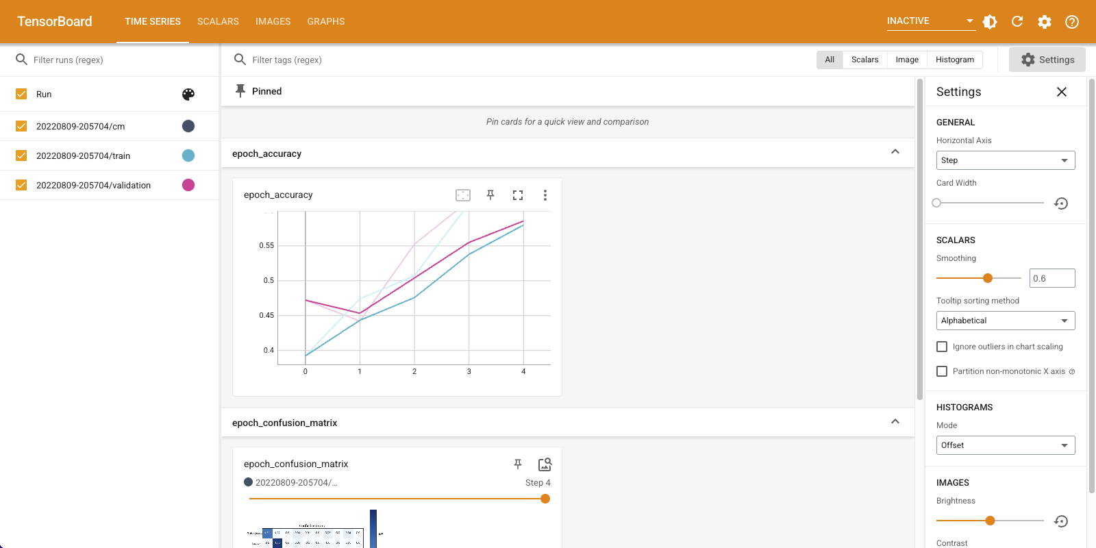
Notice that accuracy is climbing on both train and validation sets. That's a good sign. But how is the model performing on specific subsets of the data?
Scroll down the "Time Series" dashboard to visualize your logged confusion matrices. Check "Show actual image size" at the bottom of the "Settings" panel to see the confusion matrix at full size.
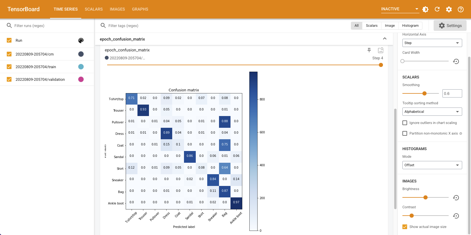
By default the dashboard shows the image summary for the last logged step or epoch. Use the slider to view earlier confusion matrices. Notice how the matrix changes significantly as training progresses, with darker squares coalescing along the diagonal, and the rest of the matrix tending toward 0 and white. This means that your classifier is improving as training progresses! Great work!
The confusion matrix shows that this simple model has some problems. Despite the great progress, Shirts, T-Shirts, and Pullovers are getting confused with each other. The model needs more work.
If you're interested, try to improve this model with a convolutional network (CNN).