
|
|
|
 View source on GitHub
|
|
This tutorial demonstrates how to create and train a sequence-to-sequence Transformer model to translate Portuguese into English. The Transformer was originally proposed in "Attention is all you need" by Vaswani et al. (2017).
Transformers are deep neural networks that replace CNNs and RNNs with self-attention. Self-attention allows Transformers to easily transmit information across the input sequences.
As explained in the Google AI Blog post:
Neural networks for machine translation typically contain an encoder reading the input sentence and generating a representation of it. A decoder then generates the output sentence word by word while consulting the representation generated by the encoder. The Transformer starts by generating initial representations, or embeddings, for each word... Then, using self-attention, it aggregates information from all of the other words, generating a new representation per word informed by the entire context, represented by the filled balls. This step is then repeated multiple times in parallel for all words, successively generating new representations.

Figure 1: Applying the Transformer to machine translation. Source: Google AI Blog.
That's a lot to digest, the goal of this tutorial is to break it down into easy to understand parts. In this tutorial you will:
- Prepare the data.
- Implement necessary components:
- Positional embeddings.
- Attention layers.
- The encoder and decoder.
- Build & train the Transformer.
- Generate translations.
- Export the model.
To get the most out of this tutorial, it helps if you know about the basics of text generation and attention mechanisms.
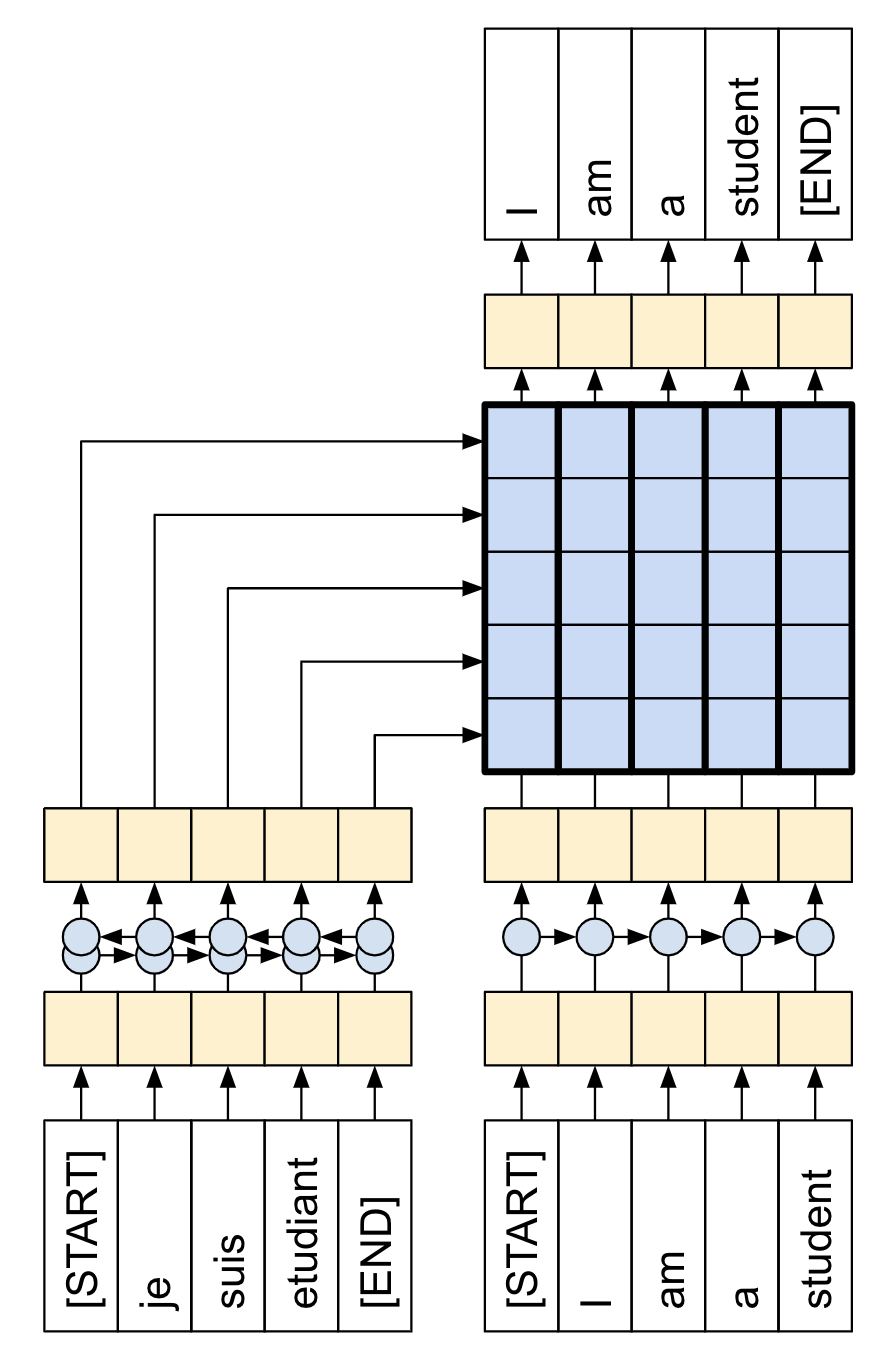
A Transformer is a sequence-to-sequence encoder-decoder model similar to the model in the NMT with attention tutorial. A single-layer Transformer takes a little more code to write, but is almost identical to that encoder-decoder RNN model. The only difference is that the RNN layers are replaced with self-attention layers. This tutorial builds a 4-layer Transformer which is larger and more powerful, but not fundamentally more complex.
| The RNN+Attention model | A 1-layer transformer |
|---|---|
|
|
After training the model in this notebook, you will be able to input a Portuguese sentence and return the English translation.

Figure 2: Visualized attention weights that you can generate at the end of this tutorial.
Why Transformers are significant
- Transformers excel at modeling sequential data, such as natural language.
- Unlike recurrent neural networks (RNNs), Transformers are parallelizable. This makes them efficient on hardware like GPUs and TPUs. The main reasons is that Transformers replaced recurrence with attention, and computations can happen simultaneously. Layer outputs can be computed in parallel, instead of a series like an RNN.
- Unlike RNNs (such as seq2seq, 2014) or convolutional neural networks (CNNs) (for example, ByteNet), Transformers are able to capture distant or long-range contexts and dependencies in the data between distant positions in the input or output sequences. Thus, longer connections can be learned. Attention allows each location to have access to the entire input at each layer, while in RNNs and CNNs, the information needs to pass through many processing steps to move a long distance, which makes it harder to learn.
- Transformers make no assumptions about the temporal/spatial relationships across the data. This is ideal for processing a set of objects (for example, StarCraft units).
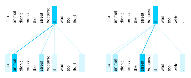
Figure 3: The encoder self-attention distribution for the word “it” from the 5th to the 6th layer of a Transformer trained on English-to-French translation (one of eight attention heads). Source: Google AI Blog.
Setup
Begin by installing TensorFlow Datasets for loading the dataset and TensorFlow Text for text preprocessing:
# Install the most re version of TensorFlow to use the improved# masking support for `tf.keras.layers.MultiHeadAttention`.apt install --allow-change-held-packages libcudnn8=8.1.0.77-1+cuda11.2pip uninstall -y -q tensorflow keras tensorflow-estimator tensorflow-textpip install protobuf~=3.20.3pip install -q tensorflow_datasetspip install -q -U tensorflow-text tensorflow
Import the necessary modules:
import logging
import time

import numpy as np
import matplotlib.pyplot as plt

import tensorflow_datasets as tfds
import tensorflow as tf

import tensorflow_text
Data handling
This section downloads the dataset and the subword tokenizer, from this tutorial, then wraps it all up in a tf.data.Dataset for training.
Download the dataset
Use TensorFlow Datasets to load the Portuguese-English translation datasetD Talks Open Translation Project. This dataset contains approximately 52,000 training, 1,200 validation and 1,800 test examples.
examples, metadata = tfds.load('ted_hrlr_translate/pt_to_en',
                               with_info=True,
                               as_supervised=True)

train_examples, val_examples = examples['train'], examples['validation']
The tf.data.Dataset object returned by TensorFlow Datasets yields pairs of text examples:
for pt_examples, en_examples in train_examples.batch(3).take(1):
  print('> Examples in Portuguese:')
  for pt in pt_examples.numpy():
    print(pt.decode('utf-8'))
  print()

  print('> Examples in English:')
  for en in en_examples.numpy():
    print(en.decode('utf-8'))
Set up the tokenizer
Now that you have loaded the dataset, you need to tokenize the text, so that each element is represented as a token or token ID (a numeric representation).
Tokenization is the process of breaking up text, into "tokens". Depending on the tokenizer, these tokens can represent sentence-pieces, words, subwords, or characters. To learn more about tokenization, visit this guide.
This tutorial uses the tokenizers built in the subword tokenizer tutorial. That tutorial optimizes two text.BertTokenizer objects (one for English, one for Portuguese) for this dataset and exports them in a TensorFlow saved_model format.
Download, extract, and import the saved_model:
model_name = 'ted_hrlr_translate_pt_en_converter'
tf.keras.utils.get_file(
    f'{model_name}.zip',
    f'https://storage.googleapis.com/download.tensorflow.org/models/{model_name}.zip',
    cache_dir='.', cache_subdir='', extract=True
)
tokenizers = tf.saved_model.load(model_name)
The tf.saved_model contains two text tokenizers, one for English and one for Portuguese. Both have the same methods:
[item for item in dir(tokenizers.en) if not item.startswith('_')]
The tokenize method converts a batch of strings to a padded-batch of token IDs. This method splits punctuation, lowercases and unicode-normalizes the input before tokenizing. That standardization is not visible here because the input data is already standardized.
print('> This is a batch of strings:')
for en in en_examples.numpy():
  print(en.decode('utf-8'))
encoded = tokenizers.en.tokenize(en_examples)

print('> This is a padded-batch of token IDs:')
for row in encoded.to_list():
  print(row)
The detokenize method attempts to convert these token IDs back to human-readable text:
round_trip = tokenizers.en.detokenize(encoded)

print('> This is human-readable text:')
for line in round_trip.numpy():
  print(line.decode('utf-8'))
The lower level lookup method converts from token-IDs to token text:
print('> This is the text split into tokens:')
tokens = tokenizers.en.lookup(encoded)
tokens
The output demonstrates the "subword" aspect of the subword tokenization.
For example, the word 'searchability' is decomposed into 'search' and '##ability', and the word 'serendipity' into 's', '##ere', '##nd', '##ip' and '##ity'.
Note that the tokenized text includes '[START]' and '[END]' tokens.
The distribution of tokens per example in the dataset is as follows:
lengths = []

for pt_examples, en_examples in train_examples.batch(1024):
  pt_tokens = tokenizers.pt.tokenize(pt_examples)
  lengths.append(pt_tokens.row_lengths())

  en_tokens = tokenizers.en.tokenize(en_examples)
  lengths.append(en_tokens.row_lengths())
  print('.', end='', flush=True)
all_lengths = np.concatenate(lengths)

plt.hist(all_lengths, np.linspace(0, 500, 101))
plt.ylim(plt.ylim())
max_length = max(all_lengths)
plt.plot([max_length, max_length], plt.ylim())
plt.title(f'Maximum tokens per example: {max_length}');
Set up a data pipeline with tf.data
The following function takes batches of text as input, and converts them to a format suitable for training.
- It tokenizes them into ragged batches.
- It trims each to be no longer than
MAX_TOKENS. - It splits the target (English) tokens into inputs and labels. These are shifted by one step so that at each input location the
labelis the id of the next token. - It converts the
RaggedTensors to padded denseTensors. - It returns an
(inputs, labels)pair.
MAX_TOKENS=128
def prepare_batch(pt, en):
    pt = tokenizers.pt.tokenize(pt)      # Output is ragged.
    pt = pt[:, :MAX_TOKENS]    # Trim to MAX_TOKENS.
    pt = pt.to_tensor()  # Convert to 0-padded dense Tensor

    en = tokenizers.en.tokenize(en)
    en = en[:, :(MAX_TOKENS+1)]
    en_inputs = en[:, :-1].to_tensor()  # Drop the [END] tokens
    en_labels = en[:, 1:].to_tensor()   # Drop the [START] tokens

    return (pt, en_inputs), en_labels
The function below converts a dataset of text examples into data of batches for training.
- It tokenizes the text, and filters out the sequences that are too long.
(The
batch/unbatchis included because the tokenizer is much more efficient on large batches). - The
cachemethod ensures that that work is only executed once. - Then
shuffleand,dense_to_ragged_batchrandomize the order and assemble batches of examples. - Finally
prefetchruns the dataset in parallel with the model to ensure that data is available when needed. See Better performance with thetf.datafor details.
BUFFER_SIZE = 20000
BATCH_SIZE = 64
def make_batches(ds):
  return (
      ds
      .shuffle(BUFFER_SIZE)
      .batch(BATCH_SIZE)
      .map(prepare_batch, tf.data.AUTOTUNE)
      .prefetch(buffer_size=tf.data.AUTOTUNE))
Test the Dataset
# Create training and validation set batches.
train_batches = make_batches(train_examples)
val_batches = make_batches(val_examples)
The resulting tf.data.Dataset objects are setup for training with Keras.
Keras Model.fit training expects (inputs, labels) pairs.
The inputs are pairs of tokenized Portuguese and English sequences, (pt, en).
The labels are the same English sequences shifted by 1.
This shift is so that at each location input en sequence, the label in the next token.
| Inputs at the bottom, labels at the top. |
|---|
|
|
This is the same as the text generation tutorial, except here you have additional input "context" (the Portuguese sequence) that the model is "conditioned" on.
This setup is called "teacher forcing" because regardless of the model's output at each timestep, it gets the true value as input for the next timestep. This is a simple and efficient way to train a text generation model. It's efficient because you don't need to run the model sequentially, the outputs at the different sequence locations can be computed in parallel.
You might have expected the input, output, pairs to simply be the Portuguese, English sequences.
Given the Portuguese sequence, the model would try to generate the English sequence.
It's possible to train a model that way. You'd need to write out the inference loop and pass the model's output back to the input. It's slower (time steps can't run in parallel), and a harder task to learn (the model can't get the end of a sentence right until it gets the beginning right), but it can give a more stable model because the model has to learn to correct its own errors during training.
for (pt, en), en_labels in train_batches.take(1):
  break

print(pt.shape)
print(en.shape)
print(en_labels.shape)
The en and en_labels are the same, just shifted by 1:
print(en[0][:10])
print(en_labels[0][:10])
Define the components
There's a lot going on inside a Transformer. The important things to remember are:
- It follows the same general pattern as a standard sequence-to-sequence model with an encoder and a decoder.
- If you work through it step by step it will all make sense.
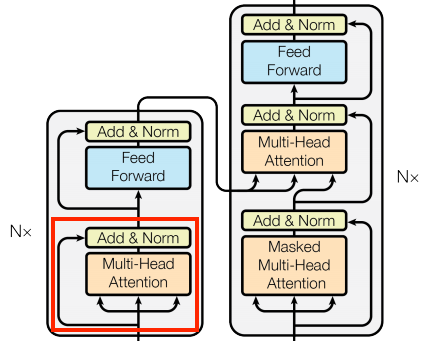
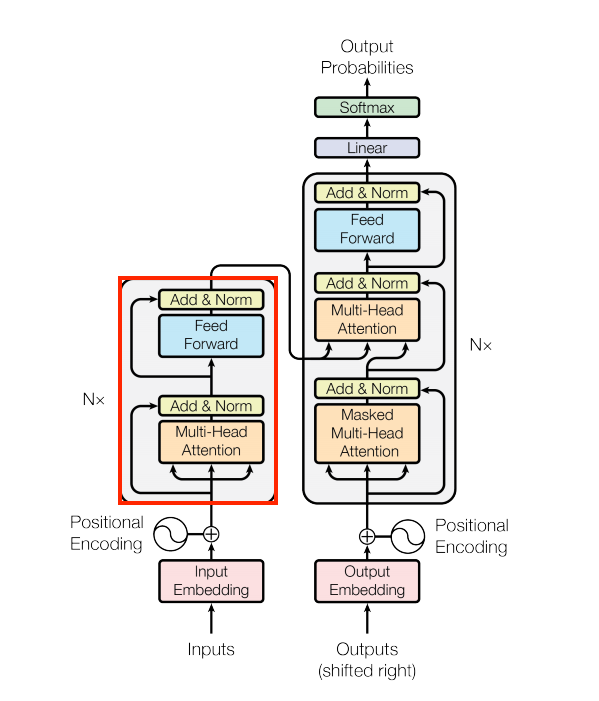
| The original Transformer diagram | A representation of a 4-layer Transformer |
|---|---|
|
|
|
Each of the components in these two diagrams will be explained as you progress through the tutorial.
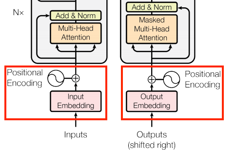
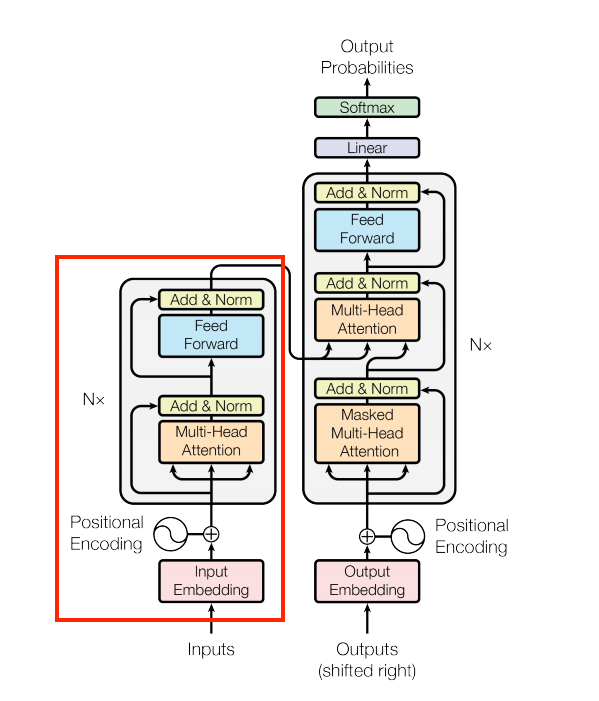
The embedding and positional encoding layer
The inputs to both the encoder and decoder use the same embedding and positional encoding logic.
| The embedding and positional encoding layer |
|---|
|
Given a sequence of tokens, both the input tokens (Portuguese) and target tokens (English) have to be converted to vectors using a tf.keras.layers.Embedding layer.
The attention layers used throughout the model see their input as a set of vectors, with no order. Since the model doesn't contain any recurrent or convolutional layers. It needs some way to identify word order, otherwise it would see the input sequence as a bag of words instance, how are you, how you are, you how are, and so on, are indistinguishable.
A Transformer adds a "Positional Encoding" to the embedding vectors. It uses a set of sines and cosines at different frequencies (across the sequence). By definition nearby elements will have similar position encodings.
The original paper uses the following formula for calculating the positional encoding:
\[\Large{PE_{(pos, 2i)} = \sin(pos / 10000^{2i / d_{model} })} \]
\[\Large{PE_{(pos, 2i+1)} = \cos(pos / 10000^{2i / d_{model} })} \]
def positional_encoding(length, depth):
  depth = depth/2

  positions = np.arange(length)[:, np.newaxis]     # (seq, 1)
  depths = np.arange(depth)[np.newaxis, :]/depth   # (1, depth)

  angle_rates = 1 / (10000**depths)         # (1, depth)
  angle_rads = positions * angle_rates      # (pos, depth)

  pos_encoding = np.concatenate(
      [np.sin(angle_rads), np.cos(angle_rads)],
      axis=-1)

  return tf.cast(pos_encoding, dtype=tf.float32)
The position encoding function is a stack of sines and cosines that vibrate at different frequencies depending on their location along the depth of the embedding vector. They vibrate across the position axis.
pos_encoding = positional_encoding(length=2048, depth=512)

# Check the shape.
print(pos_encoding.shape)

# Plot the dimensions.
plt.pcolormesh(pos_encoding.numpy().T, cmap='RdBu')
plt.ylabel('Depth')
plt.xlabel('Position')
plt.colorbar()
plt.show()
By definition these vectors align well with nearby vectors along the position axis. Below the position encoding vectors are normalized and the vector from position 1000 is compared, by dot-product, to all the others:
pos_encoding/=tf.norm(pos_encoding, axis=1, keepdims=True)
p = pos_encoding[1000]
dots = tf.einsum('pd,d -> p', pos_encoding, p)
plt.subplot(2,1,1)
plt.plot(dots)
plt.ylim([0,1])
plt.plot([950, 950, float('nan'), 1050, 1050],
         [0,1,float('nan'),0,1], color='k', label='Zoom')
plt.legend()
plt.subplot(2,1,2)
plt.plot(dots)
plt.xlim([950, 1050])
plt.ylim([0,1])
So use this to create a PositionEmbedding layer that looks-up a token's embedding vector and adds the position vector:
class PositionalEmbedding(tf.keras.layers.Layer):
  def __init__(self, vocab_size, d_model):
    super().__init__()
    self.d_model = d_model
    self.embedding = tf.keras.layers.Embedding(vocab_size, d_model, mask_zero=True)
    self.pos_encoding = positional_encoding(length=2048, depth=d_model)

  def compute_mask(self, *args, **kwargs):
    return self.embedding.compute_mask(*args, **kwargs)

  def call(self, x):
    length = tf.shape(x)[1]
    x = self.embedding(x)
    # This factor sets the relative scale of the embedding and positonal_encoding.
    x *= tf.math.sqrt(tf.cast(self.d_model, tf.float32))
    x = x + self.pos_encoding[tf.newaxis, :length, :]
    return x
embed_pt = PositionalEmbedding(vocab_size=tokenizers.pt.get_vocab_size().numpy(), d_model=512)
embed_en = PositionalEmbedding(vocab_size=tokenizers.en.get_vocab_size().numpy(), d_model=512)

pt_emb = embed_pt(pt)
en_emb = embed_en(en)
en_emb._keras_mask
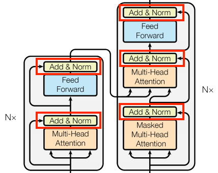
Add and normalize
| Add and normalize | |
|---|---|
|
|
These "Add & Norm" blocks are scattered throughout the model. Each one joins a residual connection and runs the result through a LayerNormalization layer.
The easiest way to organize the code is around these residual blocks. The following sections will define custom layer classes for each.
The residual "Add & Norm" blocks are included so that training is efficient. The residual connection provides a direct path for the gradient (and ensures that vectors are updated by the attention layers instead of replaced), while the normalization maintains a reasonable scale for the outputs.
The base attention layer
Attention layers are used throughout the model. These are all identical except for how the attention is configured. Each one contains a layers.MultiHeadAttention, a layers.LayerNormalization and a layers.Add.
| The base attention layer | |
|---|---|
|
|
To implement these attention layers, start with a simple base class that just contains the component layers. Each use-case will be implemented as a subclass. It's a little more code to write this way, but it keeps the intention clear.
class BaseAttention(tf.keras.layers.Layer):
  def __init__(self, **kwargs):
    super().__init__()
    self.mha = tf.keras.layers.MultiHeadAttention(**kwargs)
    self.layernorm = tf.keras.layers.LayerNormalization()
    self.add = tf.keras.layers.Add()
Attention refresher
Before you get into the specifics of each usage, here is a quick refresher on how attention works:
| The base attention layer |
|---|
|
There are two inputs:
- The query sequence; the sequence being processed; the sequence doing the attending (bottom).
- The context sequence; the sequence being attended to (left).
The output has the same shape as the query-sequence.
The common comparison is that this operation is like a dictionary lookup. A fuzzy, differentiable, vectorized dictionary lookup.
Here's a regular python dictionary, with 3 keys and 3 values being passed a single query.
d = {'color': 'blue', 'age': 22, 'type': 'pickup'}
result = d['color']
- The
querys is what you're trying to find. - The
keys what sort of information the dictionary has. - The
valueis that information.
When you look up a query in a regular dictionary, the dictionary finds the matching key, and returns its associated value.
The query either has a matching key or it doesn't.
You can imagine a fuzzy dictionary where the keys don't have to match perfectly.
If you looked up d["species"] in the dictionary above, maybe you'd want it to return "pickup" since that's the best match for the query.
An attention layer does a fuzzy lookup like this, but it's not just looking for the best key.
It combines the values based on how well the query matches each key.
How does that work? In an attention layer the query, key, and value are each vectors.
Instead of doing a hash lookup the attention layer combines the query and key vectors to determine how well they match, the "attention score".
The layer returns the average across all the values, weighted by the "attention scores".
Each location the query-sequence provides a query vector.
The context sequence acts as the dictionary. At each location in the context sequence provides a key and value vector.
The input vectors are not used directly, the layers.MultiHeadAttention layer includes layers.Dense layers to project the input vectors before using them.
The cross attention layer
At the literal center of the Transformer is the cross-attention layer. This layer connects the encoder and decoder. This layer is the most straight-forward use of attention in the model, it performs the same task as the attention block in the NMT with attention tutorial.
| The cross attention layer |
|---|
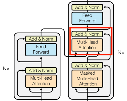
|
To implement this you pass the target sequence x as the query and the context sequence as the key/value when calling the mha layer:
class CrossAttention(BaseAttention):
  def call(self, x, context):
    attn_output, attn_scores = self.mha(
        query=x,
        key=context,
        value=context,
        return_attention_scores=True)

    # Cache the attention scores for plotting later.
    self.last_attn_scores = attn_scores

    x = self.add([x, attn_output])
    x = self.layernorm(x)

    return x
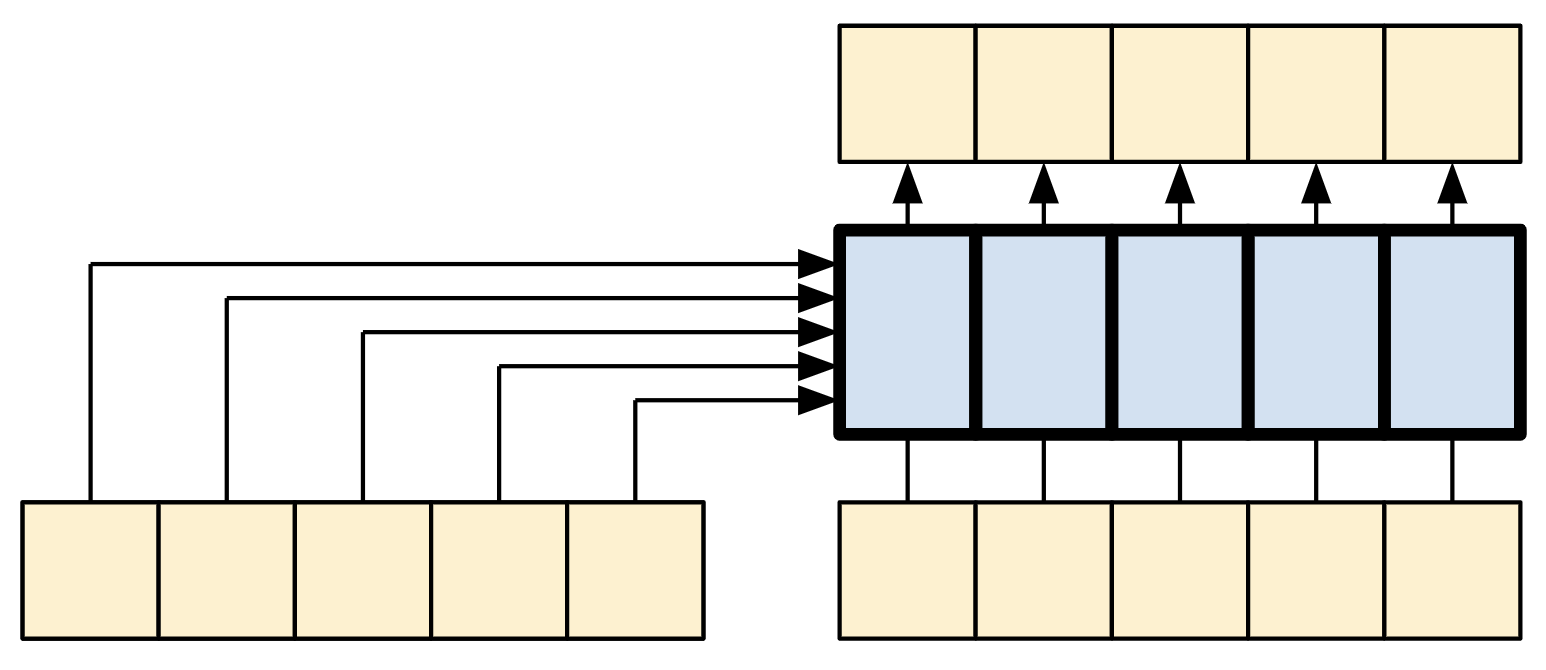
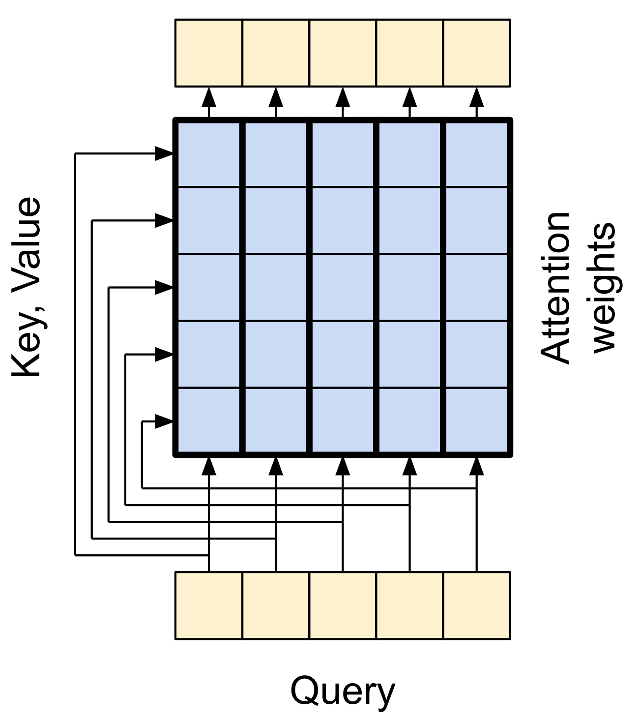
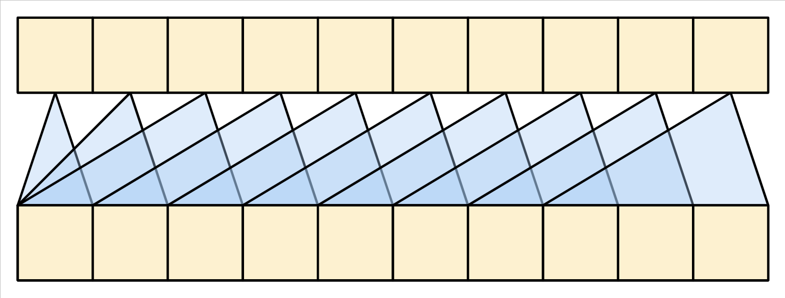
The caricature below shows how information flows through this layer. The columns represent the weighted sum over the context sequence.
For simplicity the residual connections are not shown.
| The cross attention layer |
|---|
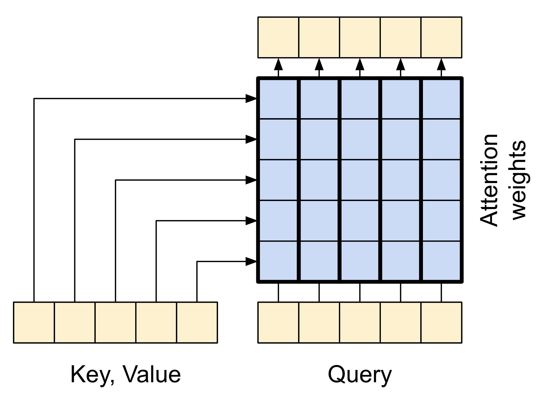
|
The output length is the length of the query sequence, and not the length of the context key/value sequence.
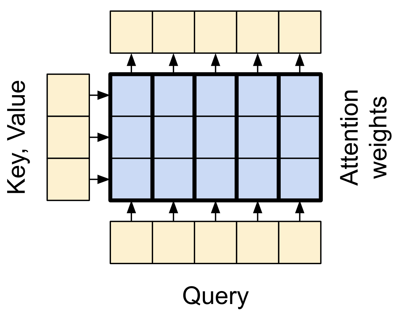
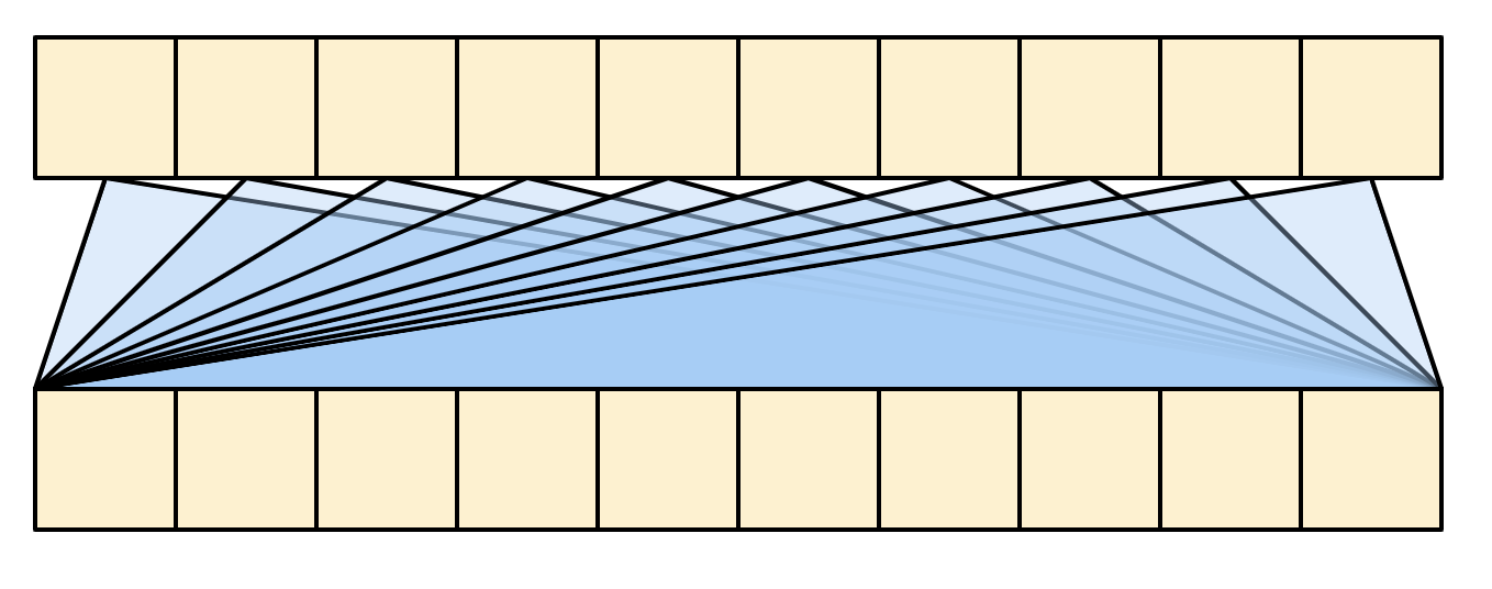
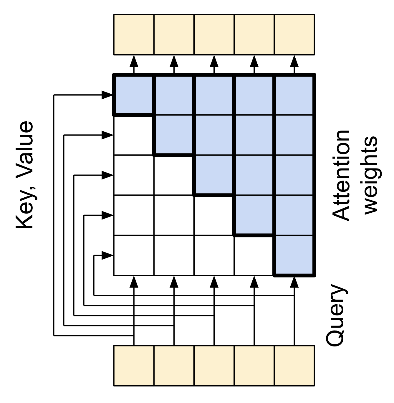
The diagram is further simplified, below. There's no need to draw the entire "Attention weights" matrix.
The point is that each query location can see all the key/value pairs in the context, but no information is exchanged between the queries.
| Each query sees the whole context. |
|---|
|
Test run it on sample inputs:
sample_ca = CrossAttention(num_heads=2, key_dim=512)

print(pt_emb.shape)
print(en_emb.shape)
print(sample_ca(en_emb, pt_emb).shape)
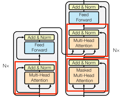
The global self-attention layer
This layer is responsible for processing the context sequence, and propagating information along its length:
| The global self-attention layer |
|---|
|
Since the context sequence is fixed while the translation is being generated, information is allowed to flow in both directions.
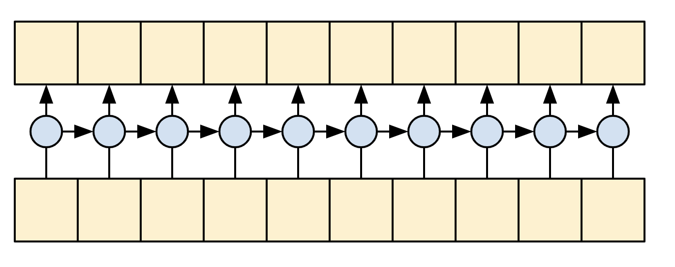
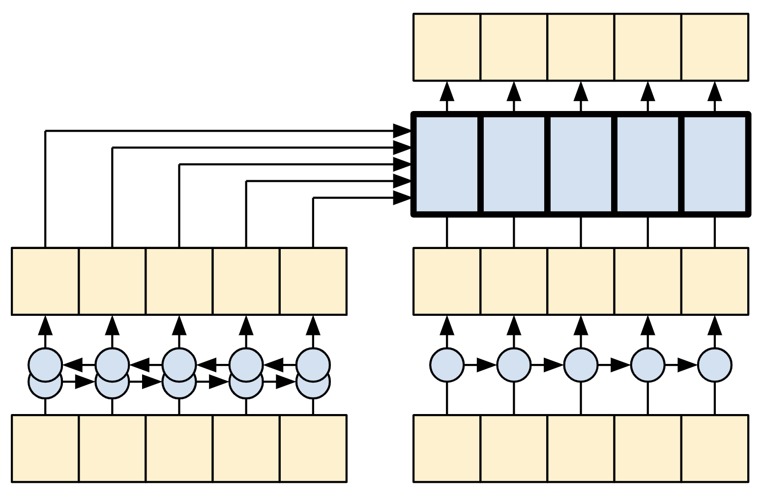
Before Transformers and self-attention, models commonly used RNNs or CNNs to do this task:
| Bidirectional RNNs and CNNs |
|---|
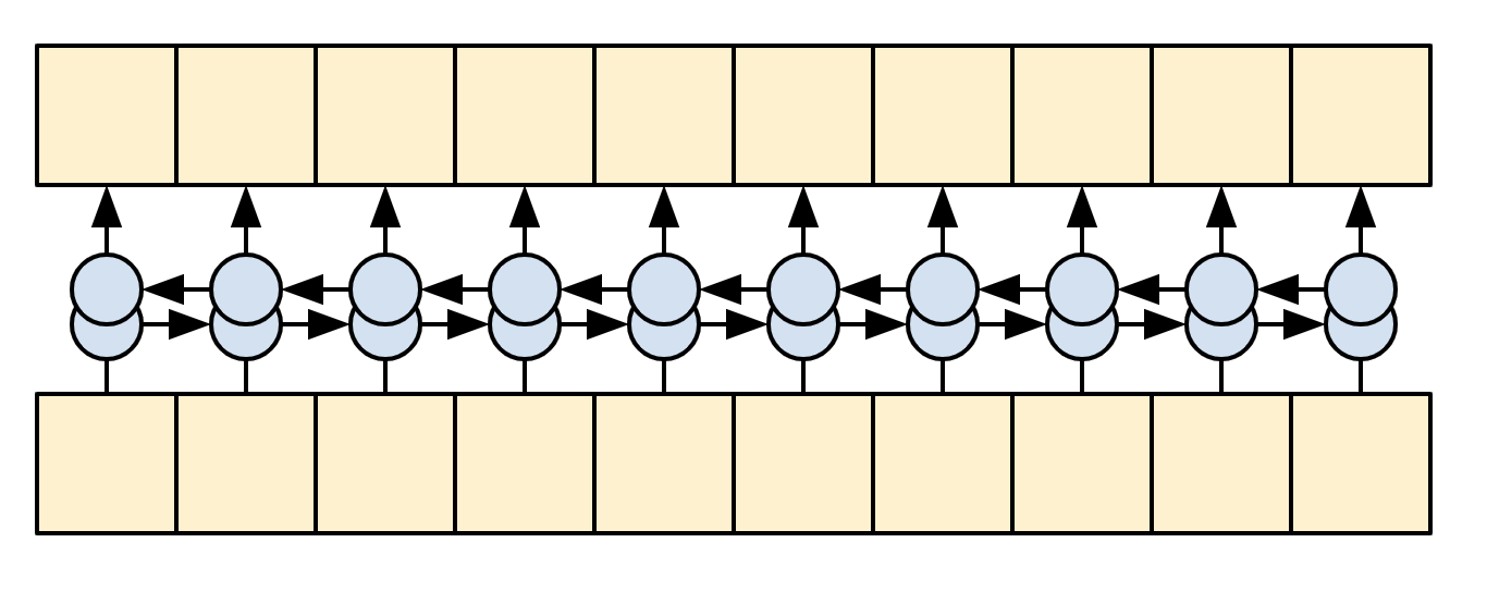
|
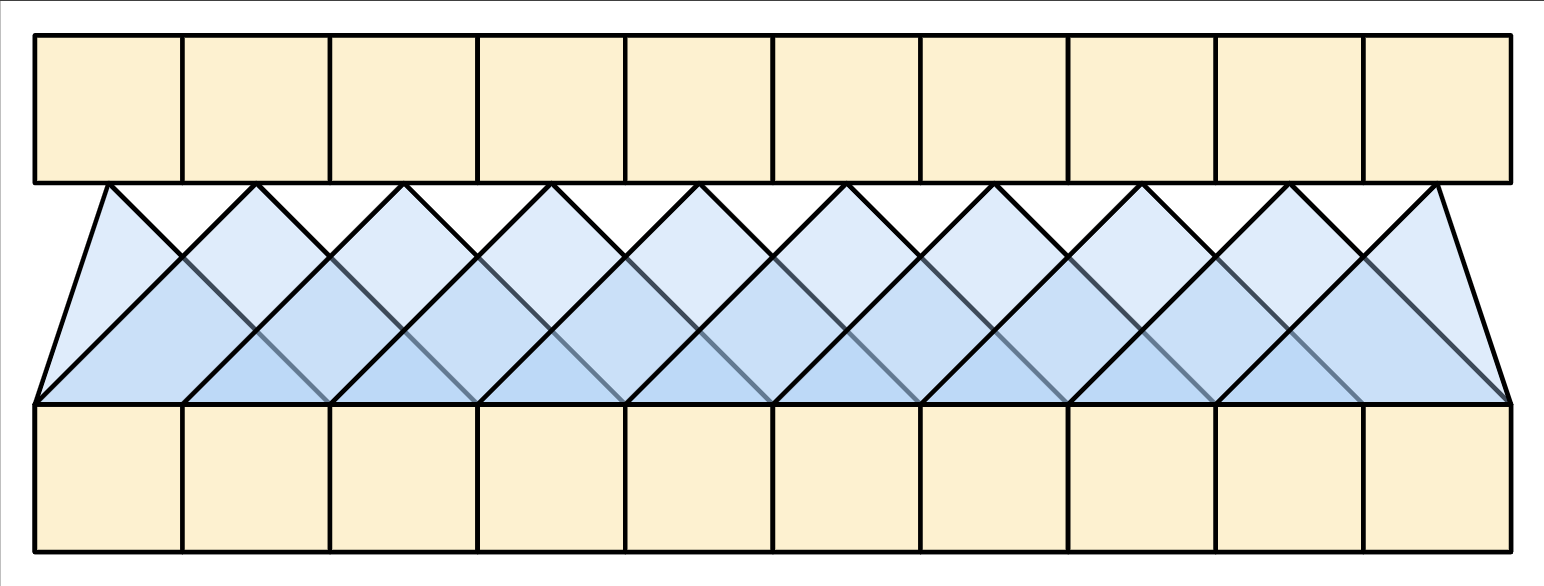
|
RNNs and CNNs have their limitations.
- The RNN allows information to flow all the way across the sequence, but it passes through many processing steps to get there (limiting gradient flow). These RNN steps have to be run sequentially and so the RNN is less able to take advantage of modern parallel devices.
- In the CNN each location can be processed in parallel, but it only provides a limited receptive field. The receptive field only grows linearly with the number of CNN layers, You need to stack a number of Convolution layers to transmit information across the sequence (Wavenet reduces this problem by using dilated convolutions).
The global self-attention layer on the other hand lets every sequence element directly access every other sequence element, with only a few operations, and all the outputs can be computed in parallel.
To implement this layer you just need to pass the target sequence, x, as both the query, and value arguments to the mha layer:
class GlobalSelfAttention(BaseAttention):
  def call(self, x):
    attn_output = self.mha(
        query=x,
        value=x,
        key=x)
    x = self.add([x, attn_output])
    x = self.layernorm(x)
    return x
sample_gsa = GlobalSelfAttention(num_heads=2, key_dim=512)

print(pt_emb.shape)
print(sample_gsa(pt_emb).shape)
Sticking with the same style as before you could draw it like this:
| The global self-attention layer |
|---|
|
Again, the residual connections are omitted for clarity.
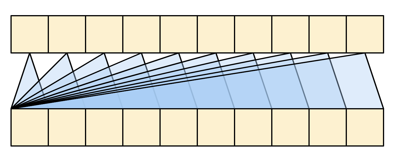
It's more compact, and just as accurate to draw it like this:
| The global self-attention layer |
|---|
|
The causal self-attention layer
This layer does a similar job as the global self-attention layer, for the output sequence:
| The causal self-attention layer |
|---|
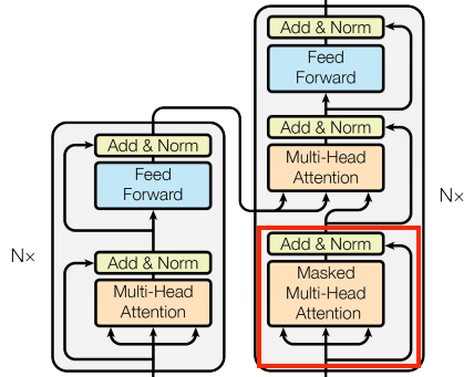
|
This needs to be handled differently from the encoder's global self-attention layer.
Like the text generation tutorial, and the NMT with attention tutorial, Transformers are an "autoregressive" model: They generate the text one token at a time and feed that output back to the input. To make this efficient, these models ensure that the output for each sequence element only depends on the previous sequence elements; the models are "causal".
A single-direction RNN is causal by definition. To make a causal convolution you just need to pad the input and shift the output so that it aligns correctly (use layers.Conv1D(padding='causal')) .
| Causal RNNs and CNNs |
|---|
|
|
A causal model is efficient in two ways:
- In training, it lets you compute loss for every location in the output sequence while executing the model just once.
- During inference, for each new token generated you only need to calculate its outputs, the outputs for the previous sequence elements can be reused.
- For an RNN you just need the RNN-state to account for previous computations (pass
return_state=Trueto the RNN layer's constructor). - For a CNN you would need to follow the approach of Fast Wavenet
- For an RNN you just need the RNN-state to account for previous computations (pass
To build a causal self-attention layer, you need to use an appropriate mask when computing the attention scores and summing the attention values.
This is taken care of automatically if you pass use_causal_mask = True to the MultiHeadAttention layer when you call it:
class CausalSelfAttention(BaseAttention):
  def call(self, x):
    attn_output = self.mha(
        query=x,
        value=x,
        key=x,
        use_causal_mask = True)
    x = self.add([x, attn_output])
    x = self.layernorm(x)
    return x
The causal mask ensures that each location only has access to the locations that come before it:
| The causal self-attention layer |
|---|
|
Again, the residual connections are omitted for simplicity.
The more compact representation of this layer would be:
| The causal self-attention layer |
|---|
|
Test out the layer:
sample_csa = CausalSelfAttention(num_heads=2, key_dim=512)

print(en_emb.shape)
print(sample_csa(en_emb).shape)
The output for early sequence elements doesn't depend on later elements, so it shouldn't matter if you trim elements before or after applying the layer:
out1 = sample_csa(embed_en(en[:, :3]))
out2 = sample_csa(embed_en(en))[:, :3]

tf.reduce_max(abs(out1 - out2)).numpy()
The feed forward network
The transformer also includes this point-wise feed-forward network in both the encoder and decoder:
| The feed forward network |
|---|
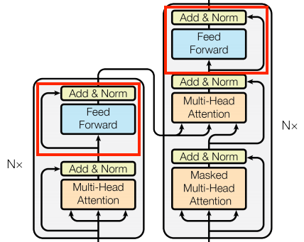
|
The network consists of two linear layers (tf.keras.layers.Dense) with a ReLU activation in-between, and a dropout layer. As with the attention layers the code here also includes the residual connection and normalization:
class FeedForward(tf.keras.layers.Layer):
  def __init__(self, d_model, dff, dropout_rate=0.1):
    super().__init__()
    self.seq = tf.keras.Sequential([
      tf.keras.layers.Dense(dff, activation='relu'),
      tf.keras.layers.Dense(d_model),
      tf.keras.layers.Dropout(dropout_rate)
    ])
    self.add = tf.keras.layers.Add()
    self.layer_norm = tf.keras.layers.LayerNormalization()

  def call(self, x):
    x = self.add([x, self.seq(x)])
    x = self.layer_norm(x)
    return x
Test the layer, the output is the same shape as the input:
sample_ffn = FeedForward(512, 2048)

print(en_emb.shape)
print(sample_ffn(en_emb).shape)
The encoder layer
The encoder contains a stack of N encoder layers. Where each EncoderLayer contains a GlobalSelfAttention and FeedForward layer:
| The encoder layer |
|---|
|
Here is the definition of the EncoderLayer:
class EncoderLayer(tf.keras.layers.Layer):
  def __init__(self,*, d_model, num_heads, dff, dropout_rate=0.1):
    super().__init__()

    self.self_attention = GlobalSelfAttention(
        num_heads=num_heads,
        key_dim=d_model,
        dropout=dropout_rate)

    self.ffn = FeedForward(d_model, dff)

  def call(self, x):
    x = self.self_attention(x)
    x = self.ffn(x)
    return x
And a quick test, the output will have the same shape as the input:
sample_encoder_layer = EncoderLayer(d_model=512, num_heads=8, dff=2048)

print(pt_emb.shape)
print(sample_encoder_layer(pt_emb).shape)
The encoder
Next build the encoder.
| The encoder |
|---|
|
The encoder consists of:
- A
PositionalEmbeddinglayer at the input. - A stack of
EncoderLayerlayers.
class Encoder(tf.keras.layers.Layer):
  def __init__(self, *, num_layers, d_model, num_heads,
               dff, vocab_size, dropout_rate=0.1):
    super().__init__()

    self.d_model = d_model
    self.num_layers = num_layers

    self.pos_embedding = PositionalEmbedding(
        vocab_size=vocab_size, d_model=d_model)

    self.enc_layers = [
        EncoderLayer(d_model=d_model,
                     num_heads=num_heads,
                     dff=dff,
                     dropout_rate=dropout_rate)
        for _ in range(num_layers)]
    self.dropout = tf.keras.layers.Dropout(dropout_rate)

  def call(self, x):
    # `x` is token-IDs shape: (batch, seq_len)
    x = self.pos_embedding(x)  # Shape `(batch_size, seq_len, d_model)`.

    # Add dropout.
    x = self.dropout(x)

    for i in range(self.num_layers):
      x = self.enc_layers[i](x)

    return x  # Shape `(batch_size, seq_len, d_model)`.
Test the encoder:
# Instantiate the encoder.
sample_encoder = Encoder(num_layers=4,
                         d_model=512,
                         num_heads=8,
                         dff=2048,
                         vocab_size=8500)

sample_encoder_output = sample_encoder(pt, training=False)

# Print the shape.
print(pt.shape)
print(sample_encoder_output.shape)  # Shape `(batch_size, input_seq_len, d_model)`.
The decoder layer
The decoder's stack is slightly more complex, with each DecoderLayer containing a CausalSelfAttention, a CrossAttention, and a FeedForward layer:
| The decoder layer |
|---|
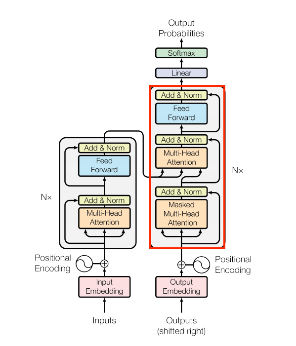
|
class DecoderLayer(tf.keras.layers.Layer):
  def __init__(self,
               *,
               d_model,
               num_heads,
               dff,
               dropout_rate=0.1):
    super(DecoderLayer, self).__init__()

    self.causal_self_attention = CausalSelfAttention(
        num_heads=num_heads,
        key_dim=d_model,
        dropout=dropout_rate)

    self.cross_attention = CrossAttention(
        num_heads=num_heads,
        key_dim=d_model,
        dropout=dropout_rate)

    self.ffn = FeedForward(d_model, dff)

  def call(self, x, context):
    x = self.causal_self_attention(x=x)
    x = self.cross_attention(x=x, context=context)

    # Cache the last attention scores for plotting later
    self.last_attn_scores = self.cross_attention.last_attn_scores

    x = self.ffn(x)  # Shape `(batch_size, seq_len, d_model)`.
    return x
Test the decoder layer:
sample_decoder_layer = DecoderLayer(d_model=512, num_heads=8, dff=2048)

sample_decoder_layer_output = sample_decoder_layer(
    x=en_emb, context=pt_emb)

print(en_emb.shape)
print(pt_emb.shape)
print(sample_decoder_layer_output.shape)  # `(batch_size, seq_len, d_model)`
The decoder
Similar to the Encoder, the Decoder consists of a PositionalEmbedding, and a stack of DecoderLayers:
| The embedding and positional encoding layer |
|---|
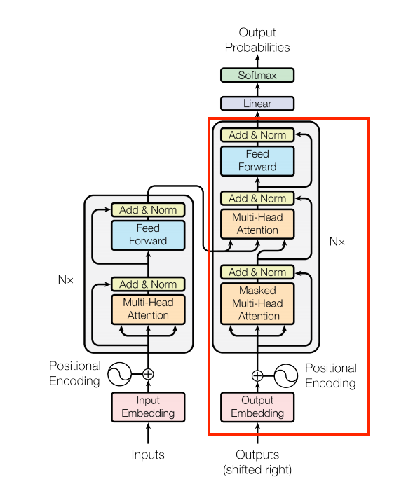
|
Define the decoder by extending tf.keras.layers.Layer:
class Decoder(tf.keras.layers.Layer):
  def __init__(self, *, num_layers, d_model, num_heads, dff, vocab_size,
               dropout_rate=0.1):
    super(Decoder, self).__init__()

    self.d_model = d_model
    self.num_layers = num_layers

    self.pos_embedding = PositionalEmbedding(vocab_size=vocab_size,
                                             d_model=d_model)
    self.dropout = tf.keras.layers.Dropout(dropout_rate)
    self.dec_layers = [
        DecoderLayer(d_model=d_model, num_heads=num_heads,
                     dff=dff, dropout_rate=dropout_rate)
        for _ in range(num_layers)]

    self.last_attn_scores = None

  def call(self, x, context):
    # `x` is token-IDs shape (batch, target_seq_len)
    x = self.pos_embedding(x)  # (batch_size, target_seq_len, d_model)

    x = self.dropout(x)

    for i in range(self.num_layers):
      x  = self.dec_layers[i](x, context)

    self.last_attn_scores = self.dec_layers[-1].last_attn_scores

    # The shape of x is (batch_size, target_seq_len, d_model).
    return x
Test the decoder:
# Instantiate the decoder.
sample_decoder = Decoder(num_layers=4,
                         d_model=512,
                         num_heads=8,
                         dff=2048,
                         vocab_size=8000)

output = sample_decoder(
    x=en,
    context=pt_emb)

# Print the shapes.
print(en.shape)
print(pt_emb.shape)
print(output.shape)
sample_decoder.last_attn_scores.shape # (batch, heads, target_seq, input_seq)
Having created the Transformer encoder and decoder, it's time to build the Transformer model and train it.
The Transformer
You now have Encoder and Decoder. To complete the Transformer model, you need to put them together and add a final linear (Dense) layer which converts the resulting vector at each location into output token probabilities.
The output of the decoder is the input to this final linear layer.
| The transformer |
|---|
|
|
A Transformer with one layer in both the Encoder and Decoder looks almost exactly like the model from the RNN+attention tutorial. A multi-layer Transformer has more layers, but is fundamentally doing the same thing.
| A 1-layer transformer | A 4-layer transformer |
|---|---|
|
|
|
| The RNN+Attention model | |
|
Create the Transformer by extending tf.keras.Model:
class Transformer(tf.keras.Model):
  def __init__(self, *, num_layers, d_model, num_heads, dff,
               input_vocab_size, target_vocab_size, dropout_rate=0.1):
    super().__init__()
    self.encoder = Encoder(num_layers=num_layers, d_model=d_model,
                           num_heads=num_heads, dff=dff,
                           vocab_size=input_vocab_size,
                           dropout_rate=dropout_rate)

    self.decoder = Decoder(num_layers=num_layers, d_model=d_model,
                           num_heads=num_heads, dff=dff,
                           vocab_size=target_vocab_size,
                           dropout_rate=dropout_rate)

    self.final_layer = tf.keras.layers.Dense(target_vocab_size)

  def call(self, inputs):
    # To use a Keras model with `.fit` you must pass all your inputs in the
    # first argument.
    context, x  = inputs

    context = self.encoder(context)  # (batch_size, context_len, d_model)

    x = self.decoder(x, context)  # (batch_size, target_len, d_model)

    # Final linear layer output.
    logits = self.final_layer(x)  # (batch_size, target_len, target_vocab_size)

    try:
      # Drop the keras mask, so it doesn't scale the losses/metrics.
      # b/250038731
      del logits._keras_mask
    except AttributeError:
      pass

    # Return the final output and the attention weights.
    return logits
Hyperparameters
To keep this example small and relatively fast, the number of layers (num_layers), the dimensionality of the embeddings (d_model), and the internal dimensionality of the FeedForward layer (dff) have been reduced.
The base model described in the original Transformer paper used num_layers=6, d_model=512, and dff=2048.
The number of self-attention heads remains the same (num_heads=8).
num_layers = 4
d_model = 128
dff = 512
num_heads = 8
dropout_rate = 0.1
Try it out
Instantiate the Transformer model:
transformer = Transformer(
    num_layers=num_layers,
    d_model=d_model,
    num_heads=num_heads,
    dff=dff,
    input_vocab_size=tokenizers.pt.get_vocab_size().numpy(),
    target_vocab_size=tokenizers.en.get_vocab_size().numpy(),
    dropout_rate=dropout_rate)
Test it:
output = transformer((pt, en))

print(en.shape)
print(pt.shape)
print(output.shape)
attn_scores = transformer.decoder.dec_layers[-1].last_attn_scores
print(attn_scores.shape)  # (batch, heads, target_seq, input_seq)
Print the summary of the model:
transformer.summary()
Training
It's time to prepare the model and start training it.
Set up the optimizer
Use the Adam optimizer with a custom learning rate scheduler according to the formula in the original Transformer paper.
\[\Large{lrate = d_{model}^{-0.5} * \min(step{\_}num^{-0.5}, step{\_}num \cdot warmup{\_}steps^{-1.5})}\]
class CustomSchedule(tf.keras.optimizers.schedules.LearningRateSchedule):
  def __init__(self, d_model, warmup_steps=4000):
    super().__init__()

    self.d_model = d_model
    self.d_model = tf.cast(self.d_model, tf.float32)

    self.warmup_steps = warmup_steps

  def __call__(self, step):
    step = tf.cast(step, dtype=tf.float32)
    arg1 = tf.math.rsqrt(step)
    arg2 = step * (self.warmup_steps ** -1.5)

    return tf.math.rsqrt(self.d_model) * tf.math.minimum(arg1, arg2)
Instantiate the optimizer (in this example it's tf.keras.optimizers.Adam):
learning_rate = CustomSchedule(d_model)

optimizer = tf.keras.optimizers.Adam(learning_rate, beta_1=0.9, beta_2=0.98,
                                     epsilon=1e-9)
Test the custom learning rate scheduler:
plt.plot(learning_rate(tf.range(40000, dtype=tf.float32)))
plt.ylabel('Learning Rate')
plt.xlabel('Train Step')
Set up the loss and metrics
Since the target sequences are padded, it is important to apply a padding mask when calculating the loss. Use the cross-entropy loss function (tf.keras.losses.SparseCategoricalCrossentropy):
def masked_loss(label, pred):
  mask = label != 0
  loss_object = tf.keras.losses.SparseCategoricalCrossentropy(
    from_logits=True, reduction='none')
  loss = loss_object(label, pred)

  mask = tf.cast(mask, dtype=loss.dtype)
  loss *= mask

  loss = tf.reduce_sum(loss)/tf.reduce_sum(mask)
  return loss


def masked_accuracy(label, pred):
  pred = tf.argmax(pred, axis=2)
  label = tf.cast(label, pred.dtype)
  match = label == pred

  mask = label != 0

  match = match & mask

  match = tf.cast(match, dtype=tf.float32)
  mask = tf.cast(mask, dtype=tf.float32)
  return tf.reduce_sum(match)/tf.reduce_sum(mask)
Train the model
With all the components ready, configure the training procedure using model.compile, and then run it with model.fit:
transformer.compile(
    loss=masked_loss,
    optimizer=optimizer,
    metrics=[masked_accuracy])
transformer.fit(train_batches,
                epochs=20,
                validation_data=val_batches)
Run inference
You can now test the model by performing a translation. The following steps are used for inference:
- Encode the input sentence using the Portuguese tokenizer (
tokenizers.pt). This is the encoder input. - The decoder input is initialized to the
[START]token. - Calculate the padding masks and the look ahead masks.
- The
decoderthen outputs the predictions by looking at theencoder outputand its own output (self-attention). - Concatenate the predicted token to the decoder input and pass it to the decoder.
- In this approach, the decoder predicts the next token based on the previous tokens it predicted.
Define the Translator class by subclassing tf.Module:
class Translator(tf.Module):
  def __init__(self, tokenizers, transformer):
    self.tokenizers = tokenizers
    self.transformer = transformer

  def __call__(self, sentence, max_length=MAX_TOKENS):
    # The input sentence is Portuguese, hence adding the `[START]` and `[END]` tokens.
    assert isinstance(sentence, tf.Tensor)
    if len(sentence.shape) == 0:
      sentence = sentence[tf.newaxis]

    sentence = self.tokenizers.pt.tokenize(sentence).to_tensor()

    encoder_input = sentence

    # As the output language is English, initialize the output with the
    # English `[START]` token.
    start_end = self.tokenizers.en.tokenize([''])[0]
    start = start_end[0][tf.newaxis]
    end = start_end[1][tf.newaxis]

    # `tf.TensorArray` is required here (instead of a Python list), so that the
    # dynamic-loop can be traced by `tf.function`.
    output_array = tf.TensorArray(dtype=tf.int64, size=0, dynamic_size=True)
    output_array = output_array.write(0, start)

    for i in tf.range(max_length):
      output = tf.transpose(output_array.stack())
      predictions = self.transformer([encoder_input, output], training=False)

      # Select the last token from the `seq_len` dimension.
      predictions = predictions[:, -1:, :]  # Shape `(batch_size, 1, vocab_size)`.

      predicted_id = tf.argmax(predictions, axis=-1)

      # Concatenate the `predicted_id` to the output which is given to the
      # decoder as its input.
      output_array = output_array.write(i+1, predicted_id[0])

      if predicted_id == end:
        break

    output = tf.transpose(output_array.stack())
    # The output shape is `(1, tokens)`.
    text = tokenizers.en.detokenize(output)[0]  # Shape: `()`.

    tokens = tokenizers.en.lookup(output)[0]

    # `tf.function` prevents us from using the attention_weights that were
    # calculated on the last iteration of the loop.
    # So, recalculate them outside the loop.
    self.transformer([encoder_input, output[:,:-1]], training=False)
    attention_weights = self.transformer.decoder.last_attn_scores

    return text, tokens, attention_weights
Create an instance of this Translator class, and try it out a few times:
translator = Translator(tokenizers, transformer)
def print_translation(sentence, tokens, ground_truth):
  print(f'{"Input:":15s}: {sentence}')
  print(f'{"Prediction":15s}: {tokens.numpy().decode("utf-8")}')
  print(f'{"Ground truth":15s}: {ground_truth}')
Example 1:
sentence = 'este é um problema que temos que resolver.'
ground_truth = 'this is a problem we have to solve .'

translated_text, translated_tokens, attention_weights = translator(
    tf.constant(sentence))
print_translation(sentence, translated_text, ground_truth)
Example 2:
sentence = 'os meus vizinhos ouviram sobre esta ideia.'
ground_truth = 'and my neighboring homes heard about this idea .'

translated_text, translated_tokens, attention_weights = translator(
    tf.constant(sentence))
print_translation(sentence, translated_text, ground_truth)
Example 3:
sentence = 'vou então muito rapidamente partilhar convosco algumas histórias de algumas coisas mágicas que aconteceram.'
ground_truth = "so i'll just share with you some stories very quickly of some magical things that have happened."

translated_text, translated_tokens, attention_weights = translator(
    tf.constant(sentence))
print_translation(sentence, translated_text, ground_truth)
Create attention plots
The Translator class you created in the previous section returns a dictionary of attention heatmaps you can use to visualize the internal working of the model.
For example:
sentence = 'este é o primeiro livro que eu fiz.'
ground_truth = "this is the first book i've ever done."

translated_text, translated_tokens, attention_weights = translator(
    tf.constant(sentence))
print_translation(sentence, translated_text, ground_truth)
Create a function that plots the attention when a token is generated:
def plot_attention_head(in_tokens, translated_tokens, attention):
  # The model didn't generate `<START>` in the output. Skip it.
  translated_tokens = translated_tokens[1:]

  ax = plt.gca()
  ax.matshow(attention)
  ax.set_xticks(range(len(in_tokens)))
  ax.set_yticks(range(len(translated_tokens)))

  labels = [label.decode('utf-8') for label in in_tokens.numpy()]
  ax.set_xticklabels(
      labels, rotation=90)

  labels = [label.decode('utf-8') for label in translated_tokens.numpy()]
  ax.set_yticklabels(labels)
head = 0
# Shape: `(batch=1, num_heads, seq_len_q, seq_len_k)`.
attention_heads = tf.squeeze(attention_weights, 0)
attention = attention_heads[head]
attention.shape
These are the input (Portuguese) tokens:
in_tokens = tf.convert_to_tensor([sentence])
in_tokens = tokenizers.pt.tokenize(in_tokens).to_tensor()
in_tokens = tokenizers.pt.lookup(in_tokens)[0]
in_tokens
And these are the output (English translation) tokens:
translated_tokens
plot_attention_head(in_tokens, translated_tokens, attention)
def plot_attention_weights(sentence, translated_tokens, attention_heads):
  in_tokens = tf.convert_to_tensor([sentence])
  in_tokens = tokenizers.pt.tokenize(in_tokens).to_tensor()
  in_tokens = tokenizers.pt.lookup(in_tokens)[0]

  fig = plt.figure(figsize=(16, 8))

  for h, head in enumerate(attention_heads):
    ax = fig.add_subplot(2, 4, h+1)

    plot_attention_head(in_tokens, translated_tokens, head)

    ax.set_xlabel(f'Head {h+1}')

  plt.tight_layout()
  plt.show()
plot_attention_weights(sentence,
                       translated_tokens,
                       attention_weights[0])
The model can handle unfamiliar words. Neither 'triceratops' nor 'encyclopédia' are in the input dataset, and the model attempts to transliterate them even without a shared vocabulary. For example:
sentence = 'Eu li sobre triceratops na enciclopédia.'
ground_truth = 'I read about triceratops in the encyclopedia.'

translated_text, translated_tokens, attention_weights = translator(
    tf.constant(sentence))
print_translation(sentence, translated_text, ground_truth)

plot_attention_weights(sentence, translated_tokens, attention_weights[0])
Export the model
You have tested the model and the inference is working. Next, you can export it as a tf.saved_model. To learn about saving and loading a model in the SavedModel format, use this guide.
Create a class called ExportTranslator by subclassing the tf.Module subclass with a tf.function on the __call__ method:
class ExportTranslator(tf.Module):
  def __init__(self, translator):
    self.translator = translator

  @tf.function(input_signature=[tf.TensorSpec(shape=[], dtype=tf.string)])
  def __call__(self, sentence):
    (result,
     tokens,
     attention_weights) = self.translator(sentence, max_length=MAX_TOKENS)

    return result
In the above tf.function only the output sentence is returned. Thanks to the non-strict execution in tf.function any unnecessary values are never computed.
Wrap translator in the newly created ExportTranslator:
translator = ExportTranslator(translator)
Since the model is decoding the predictions using tf.argmax the predictions are deterministic. The original model and one reloaded from its SavedModel should give identical predictions:
translator('este é o primeiro livro que eu fiz.').numpy()
tf.saved_model.save(translator, export_dir='translator')
reloaded = tf.saved_model.load('translator')
reloaded('este é o primeiro livro que eu fiz.').numpy()
Conclusion
In this tutorial you learned about:
- The Transformers and their significance in machine learning
- Attention, self-attention and multi-head attention
- Positional encoding with embeddings
- The encoder-decoder architecture of the original Transformer
- Masking in self-attention
- How to put it all together to translate text
The downsides of this architecture are:
- For a time-series, the output for a time-step is calculated from the entire history instead of only the inputs and current hidden-state. This may be less efficient.
- If the input has a temporal/spatial relationship, like text or images, some positional encoding must be added or the model will effectively see a bag of words.
If you want to practice, there are many things you could try with it. For example:
- Use a different dataset to train the Transformer.
- Create the "Base Transformer" or "Transformer XL" configurations from the original paper by changing the hyperparameters.
- Use the layers defined here to create an implementation of BERT
- Use Beam search to get better predictions.
There are a wide variety of Transformer-based models, many of which improve upon the 2017 version of the original Transformer with encoder-decoder, encoder-only and decoder-only architectures.
Some of these models are covered in the following research publications:
- "Efficient Transformers: a survey" (Tay et al., 2022)
- "Formal algorithms for Transformers" (Phuong and Hutter, 2022).
- T5 ("Exploring the limits of transfer learning with a unified text-to-text Transformer") (Raffel et al., 2019)
You can learn more about other models in the following Google blog posts:
If you're interested in studying how attention-based models have been applied in tasks outside of natural language processing, check out the following resources:
- Vision Transformer (ViT): Transformers for image recognition at scale
- Multi-task multitrack music transcription (MT3) with a Transformer
- Code generation with AlphaCode
- Reinforcement learning with multi-game decision Transformers
- Protein structure prediction with AlphaFold
- OptFormer: Towards universal hyperparameter optimization with Transformers