
|
|
|
 View source on GitHub
|
|
This tutorial demonstrates training a simple Convolutional Neural Network (CNN) to classify CIFAR images. Because this tutorial uses the Keras Sequential API, creating and training your model will take just a few lines of code.
Import TensorFlow
import tensorflow as tf

from tensorflow.keras import datasets, layers, models
import matplotlib.pyplot as plt
2024-08-16 03:19:29.442443: E external/local_xla/xla/stream_executor/cuda/cuda_fft.cc:485] Unable to register cuFFT factory: Attempting to register factory for plugin cuFFT when one has already been registered
2024-08-16 03:19:29.463718: E external/local_xla/xla/stream_executor/cuda/cuda_dnn.cc:8454] Unable to register cuDNN factory: Attempting to register factory for plugin cuDNN when one has already been registered
2024-08-16 03:19:29.470590: E external/local_xla/xla/stream_executor/cuda/cuda_blas.cc:1452] Unable to register cuBLAS factory: Attempting to register factory for plugin cuBLAS when one has already been registered
Download and prepare the CIFAR10 dataset
The CIFAR10 dataset contains 60,000 color images in 10 classes, with 6,000 images in each class. The dataset is divided into 50,000 training images and 10,000 testing images. The classes are mutually exclusive and there is no overlap between them.
(train_images, train_labels), (test_images, test_labels) = datasets.cifar10.load_data()

# Normalize pixel values to be between 0 and 1
train_images, test_images = train_images / 255.0, test_images / 255.0
Downloading data from https://www.cs.toronto.edu/~kriz/cifar-10-python.tar.gz
170498071/170498071 ━━━━━━━━━━━━━━━━━━━━ 4s 0us/step
Verify the data
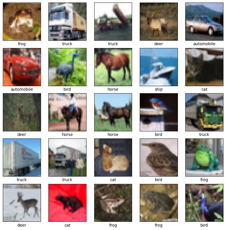
To verify that the dataset looks correct, let's plot the first 25 images from the training set and display the class name below each image:
class_names = ['airplane', 'automobile', 'bird', 'cat', 'deer',
               'dog', 'frog', 'horse', 'ship', 'truck']

plt.figure(figsize=(10,10))
for i in range(25):
    plt.subplot(5,5,i+1)
    plt.xticks([])
    plt.yticks([])
    plt.grid(False)
    plt.imshow(train_images[i])
    # The CIFAR labels happen to be arrays,
    # which is why you need the extra index
    plt.xlabel(class_names[train_labels[i][0]])
plt.show()
Create the convolutional base
The 6 lines of code below define the convolutional base using a common pattern: a stack of Conv2D and MaxPooling2D layers.
As input, a CNN takes tensors of shape (image_height, image_width, color_channels), ignoring the batch size. If you are new to these dimensions, color_channels refers to (R,G,B). In this example, you will configure your CNN to process inputs of shape (32, 32, 3), which is the format of CIFAR images. You can do this by passing the argument input_shape to your first layer.
model = models.Sequential()
model.add(layers.Conv2D(32, (3, 3), activation='relu', input_shape=(32, 32, 3)))
model.add(layers.MaxPooling2D((2, 2)))
model.add(layers.Conv2D(64, (3, 3), activation='relu'))
model.add(layers.MaxPooling2D((2, 2)))
model.add(layers.Conv2D(64, (3, 3), activation='relu'))
/tmpfs/src/tf_docs_env/lib/python3.9/site-packages/keras/src/layers/convolutional/base_conv.py:107: UserWarning: Do not pass an `input_shape`/`input_dim` argument to a layer. When using Sequential models, prefer using an `Input(shape)` object as the first layer in the model instead.
  super().__init__(activity_regularizer=activity_regularizer, **kwargs)
WARNING: All log messages before absl::InitializeLog() is called are written to STDERR
I0000 00:00:1723778380.352952  134940 cuda_executor.cc:1015] successful NUMA node read from SysFS had negative value (-1), but there must be at least one NUMA node, so returning NUMA node zero. See more at https://github.com/torvalds/linux/blob/v6.0/Documentation/ABI/testing/sysfs-bus-pci#L344-L355
I0000 00:00:1723778380.356800  134940 cuda_executor.cc:1015] successful NUMA node read from SysFS had negative value (-1), but there must be at least one NUMA node, so returning NUMA node zero. See more at https://github.com/torvalds/linux/blob/v6.0/Documentation/ABI/testing/sysfs-bus-pci#L344-L355
I0000 00:00:1723778380.360496  134940 cuda_executor.cc:1015] successful NUMA node read from SysFS had negative value (-1), but there must be at least one NUMA node, so returning NUMA node zero. See more at https://github.com/torvalds/linux/blob/v6.0/Documentation/ABI/testing/sysfs-bus-pci#L344-L355
I0000 00:00:1723778380.364197  134940 cuda_executor.cc:1015] successful NUMA node read from SysFS had negative value (-1), but there must be at least one NUMA node, so returning NUMA node zero. See more at https://github.com/torvalds/linux/blob/v6.0/Documentation/ABI/testing/sysfs-bus-pci#L344-L355
I0000 00:00:1723778380.375962  134940 cuda_executor.cc:1015] successful NUMA node read from SysFS had negative value (-1), but there must be at least one NUMA node, so returning NUMA node zero. See more at https://github.com/torvalds/linux/blob/v6.0/Documentation/ABI/testing/sysfs-bus-pci#L344-L355
I0000 00:00:1723778380.379580  134940 cuda_executor.cc:1015] successful NUMA node read from SysFS had negative value (-1), but there must be at least one NUMA node, so returning NUMA node zero. See more at https://github.com/torvalds/linux/blob/v6.0/Documentation/ABI/testing/sysfs-bus-pci#L344-L355
I0000 00:00:1723778380.382914  134940 cuda_executor.cc:1015] successful NUMA node read from SysFS had negative value (-1), but there must be at least one NUMA node, so returning NUMA node zero. See more at https://github.com/torvalds/linux/blob/v6.0/Documentation/ABI/testing/sysfs-bus-pci#L344-L355
I0000 00:00:1723778380.386363  134940 cuda_executor.cc:1015] successful NUMA node read from SysFS had negative value (-1), but there must be at least one NUMA node, so returning NUMA node zero. See more at https://github.com/torvalds/linux/blob/v6.0/Documentation/ABI/testing/sysfs-bus-pci#L344-L355
I0000 00:00:1723778380.389687  134940 cuda_executor.cc:1015] successful NUMA node read from SysFS had negative value (-1), but there must be at least one NUMA node, so returning NUMA node zero. See more at https://github.com/torvalds/linux/blob/v6.0/Documentation/ABI/testing/sysfs-bus-pci#L344-L355
I0000 00:00:1723778380.393093  134940 cuda_executor.cc:1015] successful NUMA node read from SysFS had negative value (-1), but there must be at least one NUMA node, so returning NUMA node zero. See more at https://github.com/torvalds/linux/blob/v6.0/Documentation/ABI/testing/sysfs-bus-pci#L344-L355
I0000 00:00:1723778380.396526  134940 cuda_executor.cc:1015] successful NUMA node read from SysFS had negative value (-1), but there must be at least one NUMA node, so returning NUMA node zero. See more at https://github.com/torvalds/linux/blob/v6.0/Documentation/ABI/testing/sysfs-bus-pci#L344-L355
I0000 00:00:1723778380.399979  134940 cuda_executor.cc:1015] successful NUMA node read from SysFS had negative value (-1), but there must be at least one NUMA node, so returning NUMA node zero. See more at https://github.com/torvalds/linux/blob/v6.0/Documentation/ABI/testing/sysfs-bus-pci#L344-L355
I0000 00:00:1723778381.663427  134940 cuda_executor.cc:1015] successful NUMA node read from SysFS had negative value (-1), but there must be at least one NUMA node, so returning NUMA node zero. See more at https://github.com/torvalds/linux/blob/v6.0/Documentation/ABI/testing/sysfs-bus-pci#L344-L355
I0000 00:00:1723778381.665511  134940 cuda_executor.cc:1015] successful NUMA node read from SysFS had negative value (-1), but there must be at least one NUMA node, so returning NUMA node zero. See more at https://github.com/torvalds/linux/blob/v6.0/Documentation/ABI/testing/sysfs-bus-pci#L344-L355
I0000 00:00:1723778381.667606  134940 cuda_executor.cc:1015] successful NUMA node read from SysFS had negative value (-1), but there must be at least one NUMA node, so returning NUMA node zero. See more at https://github.com/torvalds/linux/blob/v6.0/Documentation/ABI/testing/sysfs-bus-pci#L344-L355
I0000 00:00:1723778381.670244  134940 cuda_executor.cc:1015] successful NUMA node read from SysFS had negative value (-1), but there must be at least one NUMA node, so returning NUMA node zero. See more at https://github.com/torvalds/linux/blob/v6.0/Documentation/ABI/testing/sysfs-bus-pci#L344-L355
I0000 00:00:1723778381.672302  134940 cuda_executor.cc:1015] successful NUMA node read from SysFS had negative value (-1), but there must be at least one NUMA node, so returning NUMA node zero. See more at https://github.com/torvalds/linux/blob/v6.0/Documentation/ABI/testing/sysfs-bus-pci#L344-L355
I0000 00:00:1723778381.674220  134940 cuda_executor.cc:1015] successful NUMA node read from SysFS had negative value (-1), but there must be at least one NUMA node, so returning NUMA node zero. See more at https://github.com/torvalds/linux/blob/v6.0/Documentation/ABI/testing/sysfs-bus-pci#L344-L355
I0000 00:00:1723778381.676323  134940 cuda_executor.cc:1015] successful NUMA node read from SysFS had negative value (-1), but there must be at least one NUMA node, so returning NUMA node zero. See more at https://github.com/torvalds/linux/blob/v6.0/Documentation/ABI/testing/sysfs-bus-pci#L344-L355
I0000 00:00:1723778381.678321  134940 cuda_executor.cc:1015] successful NUMA node read from SysFS had negative value (-1), but there must be at least one NUMA node, so returning NUMA node zero. See more at https://github.com/torvalds/linux/blob/v6.0/Documentation/ABI/testing/sysfs-bus-pci#L344-L355
I0000 00:00:1723778381.680276  134940 cuda_executor.cc:1015] successful NUMA node read from SysFS had negative value (-1), but there must be at least one NUMA node, so returning NUMA node zero. See more at https://github.com/torvalds/linux/blob/v6.0/Documentation/ABI/testing/sysfs-bus-pci#L344-L355
I0000 00:00:1723778381.682174  134940 cuda_executor.cc:1015] successful NUMA node read from SysFS had negative value (-1), but there must be at least one NUMA node, so returning NUMA node zero. See more at https://github.com/torvalds/linux/blob/v6.0/Documentation/ABI/testing/sysfs-bus-pci#L344-L355
I0000 00:00:1723778381.684146  134940 cuda_executor.cc:1015] successful NUMA node read from SysFS had negative value (-1), but there must be at least one NUMA node, so returning NUMA node zero. See more at https://github.com/torvalds/linux/blob/v6.0/Documentation/ABI/testing/sysfs-bus-pci#L344-L355
I0000 00:00:1723778381.686151  134940 cuda_executor.cc:1015] successful NUMA node read from SysFS had negative value (-1), but there must be at least one NUMA node, so returning NUMA node zero. See more at https://github.com/torvalds/linux/blob/v6.0/Documentation/ABI/testing/sysfs-bus-pci#L344-L355
I0000 00:00:1723778381.727035  134940 cuda_executor.cc:1015] successful NUMA node read from SysFS had negative value (-1), but there must be at least one NUMA node, so returning NUMA node zero. See more at https://github.com/torvalds/linux/blob/v6.0/Documentation/ABI/testing/sysfs-bus-pci#L344-L355
I0000 00:00:1723778381.729009  134940 cuda_executor.cc:1015] successful NUMA node read from SysFS had negative value (-1), but there must be at least one NUMA node, so returning NUMA node zero. See more at https://github.com/torvalds/linux/blob/v6.0/Documentation/ABI/testing/sysfs-bus-pci#L344-L355
I0000 00:00:1723778381.731045  134940 cuda_executor.cc:1015] successful NUMA node read from SysFS had negative value (-1), but there must be at least one NUMA node, so returning NUMA node zero. See more at https://github.com/torvalds/linux/blob/v6.0/Documentation/ABI/testing/sysfs-bus-pci#L344-L355
I0000 00:00:1723778381.733079  134940 cuda_executor.cc:1015] successful NUMA node read from SysFS had negative value (-1), but there must be at least one NUMA node, so returning NUMA node zero. See more at https://github.com/torvalds/linux/blob/v6.0/Documentation/ABI/testing/sysfs-bus-pci#L344-L355
I0000 00:00:1723778381.735061  134940 cuda_executor.cc:1015] successful NUMA node read from SysFS had negative value (-1), but there must be at least one NUMA node, so returning NUMA node zero. See more at https://github.com/torvalds/linux/blob/v6.0/Documentation/ABI/testing/sysfs-bus-pci#L344-L355
I0000 00:00:1723778381.737017  134940 cuda_executor.cc:1015] successful NUMA node read from SysFS had negative value (-1), but there must be at least one NUMA node, so returning NUMA node zero. See more at https://github.com/torvalds/linux/blob/v6.0/Documentation/ABI/testing/sysfs-bus-pci#L344-L355
I0000 00:00:1723778381.739006  134940 cuda_executor.cc:1015] successful NUMA node read from SysFS had negative value (-1), but there must be at least one NUMA node, so returning NUMA node zero. See more at https://github.com/torvalds/linux/blob/v6.0/Documentation/ABI/testing/sysfs-bus-pci#L344-L355
I0000 00:00:1723778381.741008  134940 cuda_executor.cc:1015] successful NUMA node read from SysFS had negative value (-1), but there must be at least one NUMA node, so returning NUMA node zero. See more at https://github.com/torvalds/linux/blob/v6.0/Documentation/ABI/testing/sysfs-bus-pci#L344-L355
I0000 00:00:1723778381.742977  134940 cuda_executor.cc:1015] successful NUMA node read from SysFS had negative value (-1), but there must be at least one NUMA node, so returning NUMA node zero. See more at https://github.com/torvalds/linux/blob/v6.0/Documentation/ABI/testing/sysfs-bus-pci#L344-L355
I0000 00:00:1723778381.745371  134940 cuda_executor.cc:1015] successful NUMA node read from SysFS had negative value (-1), but there must be at least one NUMA node, so returning NUMA node zero. See more at https://github.com/torvalds/linux/blob/v6.0/Documentation/ABI/testing/sysfs-bus-pci#L344-L355
I0000 00:00:1723778381.747723  134940 cuda_executor.cc:1015] successful NUMA node read from SysFS had negative value (-1), but there must be at least one NUMA node, so returning NUMA node zero. See more at https://github.com/torvalds/linux/blob/v6.0/Documentation/ABI/testing/sysfs-bus-pci#L344-L355
I0000 00:00:1723778381.750088  134940 cuda_executor.cc:1015] successful NUMA node read from SysFS had negative value (-1), but there must be at least one NUMA node, so returning NUMA node zero. See more at https://github.com/torvalds/linux/blob/v6.0/Documentation/ABI/testing/sysfs-bus-pci#L344-L355
Let's display the architecture of your model so far:
model.summary()
Above, you can see that the output of every Conv2D and MaxPooling2D layer is a 3D tensor of shape (height, width, channels). The width and height dimensions tend to shrink as you go deeper in the network. The number of output channels for each Conv2D layer is controlled by the first argument (e.g., 32 or 64). Typically, as the width and height shrink, you can afford (computationally) to add more output channels in each Conv2D layer.
Add Dense layers on top
To complete the model, you will feed the last output tensor from the convolutional base (of shape (4, 4, 64)) into one or more Dense layers to perform classification. Dense layers take vectors as input (which are 1D), while the current output is a 3D tensor. First, you will flatten (or unroll) the 3D output to 1D, then add one or more Dense layers on top. CIFAR has 10 output classes, so you use a final Dense layer with 10 outputs.
model.add(layers.Flatten())
model.add(layers.Dense(64, activation='relu'))
model.add(layers.Dense(10))
Here's the complete architecture of your model:
model.summary()
The network summary shows that (4, 4, 64) outputs were flattened into vectors of shape (1024) before going through two Dense layers.
Compile and train the model
model.compile(optimizer='adam',
              loss=tf.keras.losses.SparseCategoricalCrossentropy(from_logits=True),
              metrics=['accuracy'])

history = model.fit(train_images, train_labels, epochs=10,
                    validation_data=(test_images, test_labels))
Epoch 1/10
WARNING: All log messages before absl::InitializeLog() is called are written to STDERR
I0000 00:00:1723778386.322623  135108 service.cc:146] XLA service 0x7f254c005a30 initialized for platform CUDA (this does not guarantee that XLA will be used). Devices:
I0000 00:00:1723778386.322659  135108 service.cc:154]   StreamExecutor device (0): Tesla T4, Compute Capability 7.5
I0000 00:00:1723778386.322663  135108 service.cc:154]   StreamExecutor device (1): Tesla T4, Compute Capability 7.5
I0000 00:00:1723778386.322667  135108 service.cc:154]   StreamExecutor device (2): Tesla T4, Compute Capability 7.5
I0000 00:00:1723778386.322670  135108 service.cc:154]   StreamExecutor device (3): Tesla T4, Compute Capability 7.5
70/1563 ━━━━━━━━━━━━━━━━━━━━ 3s 2ms/step - accuracy: 0.1470 - loss: 2.2585
I0000 00:00:1723778388.120198  135108 device_compiler.h:188] Compiled cluster using XLA!  This line is logged at most once for the lifetime of the process.
1563/1563 ━━━━━━━━━━━━━━━━━━━━ 10s 4ms/step - accuracy: 0.3569 - loss: 1.7377 - val_accuracy: 0.5424 - val_loss: 1.2687
Epoch 2/10
1563/1563 ━━━━━━━━━━━━━━━━━━━━ 4s 2ms/step - accuracy: 0.5721 - loss: 1.1966 - val_accuracy: 0.5967 - val_loss: 1.1490
Epoch 3/10
1563/1563 ━━━━━━━━━━━━━━━━━━━━ 4s 2ms/step - accuracy: 0.6389 - loss: 1.0240 - val_accuracy: 0.6467 - val_loss: 0.9909
Epoch 4/10
1563/1563 ━━━━━━━━━━━━━━━━━━━━ 4s 3ms/step - accuracy: 0.6764 - loss: 0.9159 - val_accuracy: 0.6715 - val_loss: 0.9493
Epoch 5/10
1563/1563 ━━━━━━━━━━━━━━━━━━━━ 4s 3ms/step - accuracy: 0.6989 - loss: 0.8506 - val_accuracy: 0.6999 - val_loss: 0.8737
Epoch 6/10
1563/1563 ━━━━━━━━━━━━━━━━━━━━ 4s 2ms/step - accuracy: 0.7275 - loss: 0.7811 - val_accuracy: 0.7032 - val_loss: 0.8687
Epoch 7/10
1563/1563 ━━━━━━━━━━━━━━━━━━━━ 4s 2ms/step - accuracy: 0.7479 - loss: 0.7160 - val_accuracy: 0.7088 - val_loss: 0.8571
Epoch 8/10
1563/1563 ━━━━━━━━━━━━━━━━━━━━ 4s 2ms/step - accuracy: 0.7650 - loss: 0.6752 - val_accuracy: 0.7035 - val_loss: 0.8852
Epoch 9/10
1563/1563 ━━━━━━━━━━━━━━━━━━━━ 4s 2ms/step - accuracy: 0.7780 - loss: 0.6372 - val_accuracy: 0.7126 - val_loss: 0.8672
Epoch 10/10
1563/1563 ━━━━━━━━━━━━━━━━━━━━ 4s 3ms/step - accuracy: 0.7946 - loss: 0.5862 - val_accuracy: 0.7163 - val_loss: 0.8550
Evaluate the model
plt.plot(history.history['accuracy'], label='accuracy')
plt.plot(history.history['val_accuracy'], label = 'val_accuracy')
plt.xlabel('Epoch')
plt.ylabel('Accuracy')
plt.ylim([0.5, 1])
plt.legend(loc='lower right')

test_loss, test_acc = model.evaluate(test_images,  test_labels, verbose=2)
313/313 - 0s - 2ms/step - accuracy: 0.7163 - loss: 0.8550
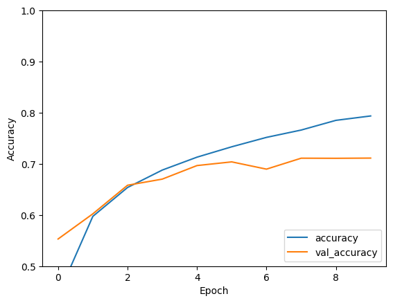
print(test_acc)
0.7163000106811523
Your simple CNN has achieved a test accuracy of over 70%. Not bad for a few lines of code! For another CNN style, check out the TensorFlow 2 quickstart for experts example that uses the Keras subclassing API and tf.GradientTape.