
|
|
|
 View source on GitHub View source on GitHub
|
|
Overview
This tutorial demonstrates data augmentation: a technique to increase the diversity of your training set by applying random (but realistic) transformations, such as image rotation.
You will learn how to apply data augmentation in two ways:
- Use the Keras preprocessing layers, such as
tf.keras.layers.Resizing,tf.keras.layers.Rescaling,tf.keras.layers.RandomFlip, andtf.keras.layers.RandomRotation. - Use the
tf.imagemethods, such astf.image.flip_left_right,tf.image.rgb_to_grayscale,tf.image.adjust_brightness,tf.image.central_crop, andtf.image.stateless_random*.
Setup
import matplotlib.pyplot as plt
import numpy as np
import tensorflow as tf
import tensorflow_datasets as tfds

from tensorflow.keras import layers
2024-07-19 05:15:47.372539: E external/local_xla/xla/stream_executor/cuda/cuda_fft.cc:485] Unable to register cuFFT factory: Attempting to register factory for plugin cuFFT when one has already been registered
2024-07-19 05:15:47.394031: E external/local_xla/xla/stream_executor/cuda/cuda_dnn.cc:8454] Unable to register cuDNN factory: Attempting to register factory for plugin cuDNN when one has already been registered
2024-07-19 05:15:47.400377: E external/local_xla/xla/stream_executor/cuda/cuda_blas.cc:1452] Unable to register cuBLAS factory: Attempting to register factory for plugin cuBLAS when one has already been registered
Download a dataset
This tutorial uses the tf_flowers dataset. For convenience, download the dataset using TensorFlow Datasets. If you would like to learn about other ways of importing data, check out the load images tutorial.
(train_ds, val_ds, test_ds), metadata = tfds.load(
    'tf_flowers',
    split=['train[:80%]', 'train[80%:90%]', 'train[90%:]'],
    with_info=True,
    as_supervised=True,
)
WARNING: All log messages before absl::InitializeLog() is called are written to STDERR
I0000 00:00:1721366151.103173   85770 cuda_executor.cc:1015] successful NUMA node read from SysFS had negative value (-1), but there must be at least one NUMA node, so returning NUMA node zero. See more at https://github.com/torvalds/linux/blob/v6.0/Documentation/ABI/testing/sysfs-bus-pci#L344-L355
I0000 00:00:1721366151.106899   85770 cuda_executor.cc:1015] successful NUMA node read from SysFS had negative value (-1), but there must be at least one NUMA node, so returning NUMA node zero. See more at https://github.com/torvalds/linux/blob/v6.0/Documentation/ABI/testing/sysfs-bus-pci#L344-L355
I0000 00:00:1721366151.110553   85770 cuda_executor.cc:1015] successful NUMA node read from SysFS had negative value (-1), but there must be at least one NUMA node, so returning NUMA node zero. See more at https://github.com/torvalds/linux/blob/v6.0/Documentation/ABI/testing/sysfs-bus-pci#L344-L355
I0000 00:00:1721366151.113677   85770 cuda_executor.cc:1015] successful NUMA node read from SysFS had negative value (-1), but there must be at least one NUMA node, so returning NUMA node zero. See more at https://github.com/torvalds/linux/blob/v6.0/Documentation/ABI/testing/sysfs-bus-pci#L344-L355
I0000 00:00:1721366151.124618   85770 cuda_executor.cc:1015] successful NUMA node read from SysFS had negative value (-1), but there must be at least one NUMA node, so returning NUMA node zero. See more at https://github.com/torvalds/linux/blob/v6.0/Documentation/ABI/testing/sysfs-bus-pci#L344-L355
I0000 00:00:1721366151.128246   85770 cuda_executor.cc:1015] successful NUMA node read from SysFS had negative value (-1), but there must be at least one NUMA node, so returning NUMA node zero. See more at https://github.com/torvalds/linux/blob/v6.0/Documentation/ABI/testing/sysfs-bus-pci#L344-L355
I0000 00:00:1721366151.131528   85770 cuda_executor.cc:1015] successful NUMA node read from SysFS had negative value (-1), but there must be at least one NUMA node, so returning NUMA node zero. See more at https://github.com/torvalds/linux/blob/v6.0/Documentation/ABI/testing/sysfs-bus-pci#L344-L355
I0000 00:00:1721366151.134385   85770 cuda_executor.cc:1015] successful NUMA node read from SysFS had negative value (-1), but there must be at least one NUMA node, so returning NUMA node zero. See more at https://github.com/torvalds/linux/blob/v6.0/Documentation/ABI/testing/sysfs-bus-pci#L344-L355
I0000 00:00:1721366151.137890   85770 cuda_executor.cc:1015] successful NUMA node read from SysFS had negative value (-1), but there must be at least one NUMA node, so returning NUMA node zero. See more at https://github.com/torvalds/linux/blob/v6.0/Documentation/ABI/testing/sysfs-bus-pci#L344-L355
I0000 00:00:1721366151.141375   85770 cuda_executor.cc:1015] successful NUMA node read from SysFS had negative value (-1), but there must be at least one NUMA node, so returning NUMA node zero. See more at https://github.com/torvalds/linux/blob/v6.0/Documentation/ABI/testing/sysfs-bus-pci#L344-L355
I0000 00:00:1721366151.144635   85770 cuda_executor.cc:1015] successful NUMA node read from SysFS had negative value (-1), but there must be at least one NUMA node, so returning NUMA node zero. See more at https://github.com/torvalds/linux/blob/v6.0/Documentation/ABI/testing/sysfs-bus-pci#L344-L355
I0000 00:00:1721366151.147465   85770 cuda_executor.cc:1015] successful NUMA node read from SysFS had negative value (-1), but there must be at least one NUMA node, so returning NUMA node zero. See more at https://github.com/torvalds/linux/blob/v6.0/Documentation/ABI/testing/sysfs-bus-pci#L344-L355
I0000 00:00:1721366152.392048   85770 cuda_executor.cc:1015] successful NUMA node read from SysFS had negative value (-1), but there must be at least one NUMA node, so returning NUMA node zero. See more at https://github.com/torvalds/linux/blob/v6.0/Documentation/ABI/testing/sysfs-bus-pci#L344-L355
I0000 00:00:1721366152.394585   85770 cuda_executor.cc:1015] successful NUMA node read from SysFS had negative value (-1), but there must be at least one NUMA node, so returning NUMA node zero. See more at https://github.com/torvalds/linux/blob/v6.0/Documentation/ABI/testing/sysfs-bus-pci#L344-L355
I0000 00:00:1721366152.396698   85770 cuda_executor.cc:1015] successful NUMA node read from SysFS had negative value (-1), but there must be at least one NUMA node, so returning NUMA node zero. See more at https://github.com/torvalds/linux/blob/v6.0/Documentation/ABI/testing/sysfs-bus-pci#L344-L355
I0000 00:00:1721366152.398787   85770 cuda_executor.cc:1015] successful NUMA node read from SysFS had negative value (-1), but there must be at least one NUMA node, so returning NUMA node zero. See more at https://github.com/torvalds/linux/blob/v6.0/Documentation/ABI/testing/sysfs-bus-pci#L344-L355
I0000 00:00:1721366152.401073   85770 cuda_executor.cc:1015] successful NUMA node read from SysFS had negative value (-1), but there must be at least one NUMA node, so returning NUMA node zero. See more at https://github.com/torvalds/linux/blob/v6.0/Documentation/ABI/testing/sysfs-bus-pci#L344-L355
I0000 00:00:1721366152.403068   85770 cuda_executor.cc:1015] successful NUMA node read from SysFS had negative value (-1), but there must be at least one NUMA node, so returning NUMA node zero. See more at https://github.com/torvalds/linux/blob/v6.0/Documentation/ABI/testing/sysfs-bus-pci#L344-L355
I0000 00:00:1721366152.405056   85770 cuda_executor.cc:1015] successful NUMA node read from SysFS had negative value (-1), but there must be at least one NUMA node, so returning NUMA node zero. See more at https://github.com/torvalds/linux/blob/v6.0/Documentation/ABI/testing/sysfs-bus-pci#L344-L355
I0000 00:00:1721366152.407060   85770 cuda_executor.cc:1015] successful NUMA node read from SysFS had negative value (-1), but there must be at least one NUMA node, so returning NUMA node zero. See more at https://github.com/torvalds/linux/blob/v6.0/Documentation/ABI/testing/sysfs-bus-pci#L344-L355
I0000 00:00:1721366152.409188   85770 cuda_executor.cc:1015] successful NUMA node read from SysFS had negative value (-1), but there must be at least one NUMA node, so returning NUMA node zero. See more at https://github.com/torvalds/linux/blob/v6.0/Documentation/ABI/testing/sysfs-bus-pci#L344-L355
I0000 00:00:1721366152.411129   85770 cuda_executor.cc:1015] successful NUMA node read from SysFS had negative value (-1), but there must be at least one NUMA node, so returning NUMA node zero. See more at https://github.com/torvalds/linux/blob/v6.0/Documentation/ABI/testing/sysfs-bus-pci#L344-L355
I0000 00:00:1721366152.413098   85770 cuda_executor.cc:1015] successful NUMA node read from SysFS had negative value (-1), but there must be at least one NUMA node, so returning NUMA node zero. See more at https://github.com/torvalds/linux/blob/v6.0/Documentation/ABI/testing/sysfs-bus-pci#L344-L355
I0000 00:00:1721366152.415071   85770 cuda_executor.cc:1015] successful NUMA node read from SysFS had negative value (-1), but there must be at least one NUMA node, so returning NUMA node zero. See more at https://github.com/torvalds/linux/blob/v6.0/Documentation/ABI/testing/sysfs-bus-pci#L344-L355
I0000 00:00:1721366152.453504   85770 cuda_executor.cc:1015] successful NUMA node read from SysFS had negative value (-1), but there must be at least one NUMA node, so returning NUMA node zero. See more at https://github.com/torvalds/linux/blob/v6.0/Documentation/ABI/testing/sysfs-bus-pci#L344-L355
I0000 00:00:1721366152.455524   85770 cuda_executor.cc:1015] successful NUMA node read from SysFS had negative value (-1), but there must be at least one NUMA node, so returning NUMA node zero. See more at https://github.com/torvalds/linux/blob/v6.0/Documentation/ABI/testing/sysfs-bus-pci#L344-L355
I0000 00:00:1721366152.457568   85770 cuda_executor.cc:1015] successful NUMA node read from SysFS had negative value (-1), but there must be at least one NUMA node, so returning NUMA node zero. See more at https://github.com/torvalds/linux/blob/v6.0/Documentation/ABI/testing/sysfs-bus-pci#L344-L355
I0000 00:00:1721366152.459614   85770 cuda_executor.cc:1015] successful NUMA node read from SysFS had negative value (-1), but there must be at least one NUMA node, so returning NUMA node zero. See more at https://github.com/torvalds/linux/blob/v6.0/Documentation/ABI/testing/sysfs-bus-pci#L344-L355
I0000 00:00:1721366152.462372   85770 cuda_executor.cc:1015] successful NUMA node read from SysFS had negative value (-1), but there must be at least one NUMA node, so returning NUMA node zero. See more at https://github.com/torvalds/linux/blob/v6.0/Documentation/ABI/testing/sysfs-bus-pci#L344-L355
I0000 00:00:1721366152.464351   85770 cuda_executor.cc:1015] successful NUMA node read from SysFS had negative value (-1), but there must be at least one NUMA node, so returning NUMA node zero. See more at https://github.com/torvalds/linux/blob/v6.0/Documentation/ABI/testing/sysfs-bus-pci#L344-L355
I0000 00:00:1721366152.466338   85770 cuda_executor.cc:1015] successful NUMA node read from SysFS had negative value (-1), but there must be at least one NUMA node, so returning NUMA node zero. See more at https://github.com/torvalds/linux/blob/v6.0/Documentation/ABI/testing/sysfs-bus-pci#L344-L355
I0000 00:00:1721366152.468345   85770 cuda_executor.cc:1015] successful NUMA node read from SysFS had negative value (-1), but there must be at least one NUMA node, so returning NUMA node zero. See more at https://github.com/torvalds/linux/blob/v6.0/Documentation/ABI/testing/sysfs-bus-pci#L344-L355
I0000 00:00:1721366152.470510   85770 cuda_executor.cc:1015] successful NUMA node read from SysFS had negative value (-1), but there must be at least one NUMA node, so returning NUMA node zero. See more at https://github.com/torvalds/linux/blob/v6.0/Documentation/ABI/testing/sysfs-bus-pci#L344-L355
I0000 00:00:1721366152.472916   85770 cuda_executor.cc:1015] successful NUMA node read from SysFS had negative value (-1), but there must be at least one NUMA node, so returning NUMA node zero. See more at https://github.com/torvalds/linux/blob/v6.0/Documentation/ABI/testing/sysfs-bus-pci#L344-L355
I0000 00:00:1721366152.475305   85770 cuda_executor.cc:1015] successful NUMA node read from SysFS had negative value (-1), but there must be at least one NUMA node, so returning NUMA node zero. See more at https://github.com/torvalds/linux/blob/v6.0/Documentation/ABI/testing/sysfs-bus-pci#L344-L355
I0000 00:00:1721366152.477750   85770 cuda_executor.cc:1015] successful NUMA node read from SysFS had negative value (-1), but there must be at least one NUMA node, so returning NUMA node zero. See more at https://github.com/torvalds/linux/blob/v6.0/Documentation/ABI/testing/sysfs-bus-pci#L344-L355
The flowers dataset has five classes.
num_classes = metadata.features['label'].num_classes
print(num_classes)
5
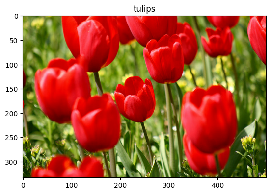
Let's retrieve an image from the dataset and use it to demonstrate data augmentation.
get_label_name = metadata.features['label'].int2str

image, label = next(iter(train_ds))
_ = plt.imshow(image)
_ = plt.title(get_label_name(label))
2024-07-19 05:15:54.153080: W tensorflow/core/kernels/data/cache_dataset_ops.cc:913] The calling iterator did not fully read the dataset being cached. In order to avoid unexpected truncation of the dataset, the partially cached contents of the dataset will be discarded. This can happen if you have an input pipeline similar to `dataset.cache().take(k).repeat()`. You should use `dataset.take(k).cache().repeat()` instead.
Use Keras preprocessing layers
Resizing and rescaling
You can use the Keras preprocessing layers to resize your images to a consistent shape (with tf.keras.layers.Resizing), and to rescale pixel values (with tf.keras.layers.Rescaling).
IMG_SIZE = 180

resize_and_rescale = tf.keras.Sequential([
  layers.Resizing(IMG_SIZE, IMG_SIZE),
  layers.Rescaling(1./255)
])
You can visualize the result of applying these layers to an image.
result = resize_and_rescale(image)
_ = plt.imshow(result)
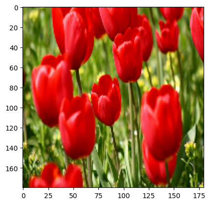
Verify that the pixels are in the [0, 1] range:
print("Min and max pixel values:", result.numpy().min(), result.numpy().max())
Min and max pixel values: 0.0 1.0
Data augmentation
You can use the Keras preprocessing layers for data augmentation as well, such as tf.keras.layers.RandomFlip and tf.keras.layers.RandomRotation.
Let's create a few preprocessing layers and apply them repeatedly to the same image.
data_augmentation = tf.keras.Sequential([
  layers.RandomFlip("horizontal_and_vertical"),
  layers.RandomRotation(0.2),
])
# Add the image to a batch.
image = tf.cast(tf.expand_dims(image, 0), tf.float32)
plt.figure(figsize=(10, 10))
for i in range(9):
  augmented_image = data_augmentation(image)
  ax = plt.subplot(3, 3, i + 1)
  plt.imshow(augmented_image[0])
  plt.axis("off")
WARNING:matplotlib.image:Clipping input data to the valid range for imshow with RGB data ([0..1] for floats or [0..255] for integers). Got range [0.0..255.0].
WARNING:matplotlib.image:Clipping input data to the valid range for imshow with RGB data ([0..1] for floats or [0..255] for integers). Got range [0.0..255.0].
WARNING:matplotlib.image:Clipping input data to the valid range for imshow with RGB data ([0..1] for floats or [0..255] for integers). Got range [0.0..255.0].
WARNING:matplotlib.image:Clipping input data to the valid range for imshow with RGB data ([0..1] for floats or [0..255] for integers). Got range [0.0..255.0].
WARNING:matplotlib.image:Clipping input data to the valid range for imshow with RGB data ([0..1] for floats or [0..255] for integers). Got range [0.0..255.0].
WARNING:matplotlib.image:Clipping input data to the valid range for imshow with RGB data ([0..1] for floats or [0..255] for integers). Got range [0.0..255.0].
WARNING:matplotlib.image:Clipping input data to the valid range for imshow with RGB data ([0..1] for floats or [0..255] for integers). Got range [0.0..255.0].
WARNING:matplotlib.image:Clipping input data to the valid range for imshow with RGB data ([0..1] for floats or [0..255] for integers). Got range [0.0..255.0].
WARNING:matplotlib.image:Clipping input data to the valid range for imshow with RGB data ([0..1] for floats or [0..255] for integers). Got range [0.0..255.0].
There are a variety of preprocessing layers you can use for data augmentation including tf.keras.layers.RandomContrast, tf.keras.layers.RandomCrop, tf.keras.layers.RandomZoom, and others.
Two options to use the Keras preprocessing layers
There are two ways you can use these preprocessing layers, with important trade-offs.
Option 1: Make the preprocessing layers part of your model
model = tf.keras.Sequential([
  # Add the preprocessing layers you created earlier.
  resize_and_rescale,
  data_augmentation,
  layers.Conv2D(16, 3, padding='same', activation='relu'),
  layers.MaxPooling2D(),
  # Rest of your model.
])
There are two important points to be aware of in this case:
Data augmentation will run on-device, synchronously with the rest of your layers, and benefit from GPU acceleration.
When you export your model using
model.save, the preprocessing layers will be saved along with the rest of your model. If you later deploy this model, it will automatically standardize images (according to the configuration of your layers). This can save you from the effort of having to reimplement that logic server-side.
Option 2: Apply the preprocessing layers to your dataset
aug_ds = train_ds.map(
  lambda x, y: (resize_and_rescale(x, training=True), y))
With this approach, you use Dataset.map to create a dataset that yields batches of augmented images. In this case:
- Data augmentation will happen asynchronously on the CPU, and is non-blocking. You can overlap the training of your model on the GPU with data preprocessing, using
Dataset.prefetch, shown below. - In this case the preprocessing layers will not be exported with the model when you call
Model.save. You will need to attach them to your model before saving it or reimplement them server-side. After training, you can attach the preprocessing layers before export.
You can find an example of the first option in the Image classification tutorial. Let's demonstrate the second option here.
Apply the preprocessing layers to the datasets
Configure the training, validation, and test datasets with the Keras preprocessing layers you created earlier. You will also configure the datasets for performance, using parallel reads and buffered prefetching to yield batches from disk without I/O become blocking. (Learn more dataset performance in the Better performance with the tf.data API guide.)
batch_size = 32
AUTOTUNE = tf.data.AUTOTUNE

def prepare(ds, shuffle=False, augment=False):
  # Resize and rescale all datasets.
  ds = ds.map(lambda x, y: (resize_and_rescale(x), y),
              num_parallel_calls=AUTOTUNE)

  if shuffle:
    ds = ds.shuffle(1000)

  # Batch all datasets.
  ds = ds.batch(batch_size)

  # Use data augmentation only on the training set.
  if augment:
    ds = ds.map(lambda x, y: (data_augmentation(x, training=True), y),
                num_parallel_calls=AUTOTUNE)

  # Use buffered prefetching on all datasets.
  return ds.prefetch(buffer_size=AUTOTUNE)
train_ds = prepare(train_ds, shuffle=True, augment=True)
val_ds = prepare(val_ds)
test_ds = prepare(test_ds)
Train a model
For completeness, you will now train a model using the datasets you have just prepared.
The Sequential model consists of three convolution blocks (tf.keras.layers.Conv2D) with a max pooling layer (tf.keras.layers.MaxPooling2D) in each of them. There's a fully-connected layer (tf.keras.layers.Dense) with 128 units on top of it that is activated by a ReLU activation function ('relu'). This model has not been tuned for accuracy (the goal is to show you the mechanics).
model = tf.keras.Sequential([
  layers.Conv2D(16, 3, padding='same', activation='relu'),
  layers.MaxPooling2D(),
  layers.Conv2D(32, 3, padding='same', activation='relu'),
  layers.MaxPooling2D(),
  layers.Conv2D(64, 3, padding='same', activation='relu'),
  layers.MaxPooling2D(),
  layers.Flatten(),
  layers.Dense(128, activation='relu'),
  layers.Dense(num_classes)
])
Choose the tf.keras.optimizers.Adam optimizer and tf.keras.losses.SparseCategoricalCrossentropy loss function. To view training and validation accuracy for each training epoch, pass the metrics argument to Model.compile.
model.compile(optimizer='adam',
              loss=tf.keras.losses.SparseCategoricalCrossentropy(from_logits=True),
              metrics=['accuracy'])
Train for a few epochs:
epochs=5
history = model.fit(
  train_ds,
  validation_data=val_ds,
  epochs=epochs
)
Epoch 1/5
WARNING: All log messages before absl::InitializeLog() is called are written to STDERR
I0000 00:00:1721366158.915097   85932 service.cc:146] XLA service 0x7f2fa805d180 initialized for platform CUDA (this does not guarantee that XLA will be used). Devices:
I0000 00:00:1721366158.915147   85932 service.cc:154]   StreamExecutor device (0): Tesla T4, Compute Capability 7.5
I0000 00:00:1721366158.915153   85932 service.cc:154]   StreamExecutor device (1): Tesla T4, Compute Capability 7.5
I0000 00:00:1721366158.915158   85932 service.cc:154]   StreamExecutor device (2): Tesla T4, Compute Capability 7.5
I0000 00:00:1721366158.915162   85932 service.cc:154]   StreamExecutor device (3): Tesla T4, Compute Capability 7.5
E0000 00:00:1721366160.445074   85932 gpu_timer.cc:183] Delay kernel timed out: measured time has sub-optimal accuracy. There may be a missing warmup execution, please investigate in Nsight Systems.
E0000 00:00:1721366160.585228   85932 gpu_timer.cc:183] Delay kernel timed out: measured time has sub-optimal accuracy. There may be a missing warmup execution, please investigate in Nsight Systems.
10/92 ━━━━━━━━━━━━━━━━━━━━ 1s 19ms/step - accuracy: 0.2324 - loss: 3.1396
I0000 00:00:1721366162.210771   85932 device_compiler.h:188] Compiled cluster using XLA!  This line is logged at most once for the lifetime of the process.
91/92 ━━━━━━━━━━━━━━━━━━━━ 0s 19ms/step - accuracy: 0.3021 - loss: 1.8969
E0000 00:00:1721366164.729563   85932 gpu_timer.cc:183] Delay kernel timed out: measured time has sub-optimal accuracy. There may be a missing warmup execution, please investigate in Nsight Systems.
E0000 00:00:1721366164.868449   85932 gpu_timer.cc:183] Delay kernel timed out: measured time has sub-optimal accuracy. There may be a missing warmup execution, please investigate in Nsight Systems.
92/92 ━━━━━━━━━━━━━━━━━━━━ 19s 140ms/step - accuracy: 0.3038 - loss: 1.8879 - val_accuracy: 0.4632 - val_loss: 1.2882
Epoch 2/5
92/92 ━━━━━━━━━━━━━━━━━━━━ 2s 20ms/step - accuracy: 0.5272 - loss: 1.1600 - val_accuracy: 0.6049 - val_loss: 1.0506
Epoch 3/5
92/92 ━━━━━━━━━━━━━━━━━━━━ 2s 21ms/step - accuracy: 0.5664 - loss: 1.0508 - val_accuracy: 0.5722 - val_loss: 1.0648
Epoch 4/5
92/92 ━━━━━━━━━━━━━━━━━━━━ 2s 20ms/step - accuracy: 0.6072 - loss: 0.9941 - val_accuracy: 0.6512 - val_loss: 1.0124
Epoch 5/5
92/92 ━━━━━━━━━━━━━━━━━━━━ 2s 20ms/step - accuracy: 0.6219 - loss: 0.9591 - val_accuracy: 0.6703 - val_loss: 0.9144
loss, acc = model.evaluate(test_ds)
print("Accuracy", acc)
12/12 ━━━━━━━━━━━━━━━━━━━━ 1s 6ms/step - accuracy: 0.6221 - loss: 0.9107
Accuracy 0.6430517435073853
Custom data augmentation
You can also create custom data augmentation layers.
This section of the tutorial shows two ways of doing so:
- First, you will create a
tf.keras.layers.Lambdalayer. This is a good way to write concise code. - Next, you will write a new layer via subclassing, which gives you more control.
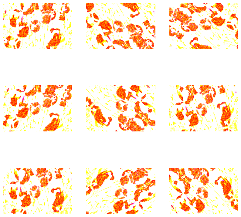
Both layers will randomly invert the colors in an image, according to some probability.
def random_invert_img(x, p=0.5):
  if  tf.random.uniform([]) < p:
    x = (255-x)
  else:
    x
  return x
def random_invert(factor=0.5):
  return layers.Lambda(lambda x: random_invert_img(x, factor))

random_invert = random_invert()
plt.figure(figsize=(10, 10))
for i in range(9):
  augmented_image = random_invert(image)
  ax = plt.subplot(3, 3, i + 1)
  plt.imshow(augmented_image[0].numpy().astype("uint8"))
  plt.axis("off")
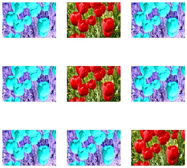
Next, implement a custom layer by subclassing:
class RandomInvert(layers.Layer):
  def __init__(self, factor=0.5, **kwargs):
    super().__init__(**kwargs)
    self.factor = factor

  def call(self, x):
    return random_invert_img(x)
_ = plt.imshow(RandomInvert()(image)[0])
WARNING:matplotlib.image:Clipping input data to the valid range for imshow with RGB data ([0..1] for floats or [0..255] for integers). Got range [0.0..255.0].
Both of these layers can be used as described in options 1 and 2 above.
Using tf.image
The above Keras preprocessing utilities are convenient. But, for finer control, you can write your own data augmentation pipelines or layers using tf.data and tf.image. (You may also want to check out TensorFlow Addons Image: Operations and TensorFlow I/O: Color Space Conversions.)
Since the flowers dataset was previously configured with data augmentation, let's reimport it to start fresh:
(train_ds, val_ds, test_ds), metadata = tfds.load(
    'tf_flowers',
    split=['train[:80%]', 'train[80%:90%]', 'train[90%:]'],
    with_info=True,
    as_supervised=True,
)
Retrieve an image to work with:
image, label = next(iter(train_ds))
_ = plt.imshow(image)
_ = plt.title(get_label_name(label))
2024-07-19 05:16:27.111848: W tensorflow/core/kernels/data/cache_dataset_ops.cc:913] The calling iterator did not fully read the dataset being cached. In order to avoid unexpected truncation of the dataset, the partially cached contents of the dataset will be discarded. This can happen if you have an input pipeline similar to `dataset.cache().take(k).repeat()`. You should use `dataset.take(k).cache().repeat()` instead.

Let's use the following function to visualize and compare the original and augmented images side-by-side:
def visualize(original, augmented):
  fig = plt.figure()
  plt.subplot(1,2,1)
  plt.title('Original image')
  plt.imshow(original)

  plt.subplot(1,2,2)
  plt.title('Augmented image')
  plt.imshow(augmented)
Data augmentation
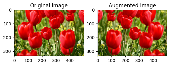
Flip an image
Flip an image either vertically or horizontally with tf.image.flip_left_right:
flipped = tf.image.flip_left_right(image)
visualize(image, flipped)
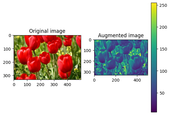
Grayscale an image
You can grayscale an image with tf.image.rgb_to_grayscale:
grayscaled = tf.image.rgb_to_grayscale(image)
visualize(image, tf.squeeze(grayscaled))
_ = plt.colorbar()
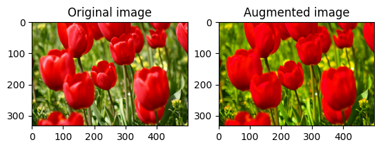
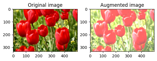
Saturate an image
Saturate an image with tf.image.adjust_saturation by providing a saturation factor:
saturated = tf.image.adjust_saturation(image, 3)
visualize(image, saturated)
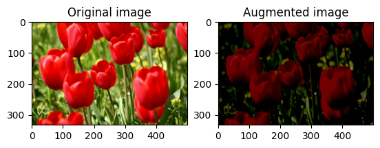
Change image brightness
Change the brightness of image with tf.image.adjust_brightness by providing a brightness factor:
bright = tf.image.adjust_brightness(image, 0.4)
visualize(image, bright)
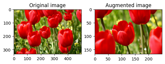
Center crop an image
Crop the image from center up to the image part you desire using tf.image.central_crop:
cropped = tf.image.central_crop(image, central_fraction=0.5)
visualize(image, cropped)
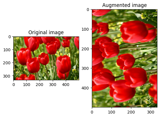
Rotate an image
Rotate an image by 90 degrees with tf.image.rot90:
rotated = tf.image.rot90(image)
visualize(image, rotated)
Random transformations
Applying random transformations to the images can further help generalize and expand the dataset. The current tf.image API provides eight such random image operations (ops):
tf.image.stateless_random_brightnesstf.image.stateless_random_contrasttf.image.stateless_random_croptf.image.stateless_random_flip_left_righttf.image.stateless_random_flip_up_downtf.image.stateless_random_huetf.image.stateless_random_jpeg_qualitytf.image.stateless_random_saturation
These random image ops are purely functional: the output only depends on the input. This makes them simple to use in high performance, deterministic input pipelines. They require a seed value be input each step. Given the same seed, they return the same results independent of how many times they are called.
In the following sections, you will:
- Go over examples of using random image operations to transform an image.
- Demonstrate how to apply random transformations to a training dataset.
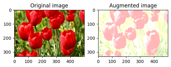
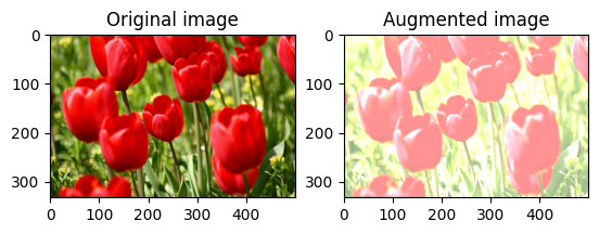
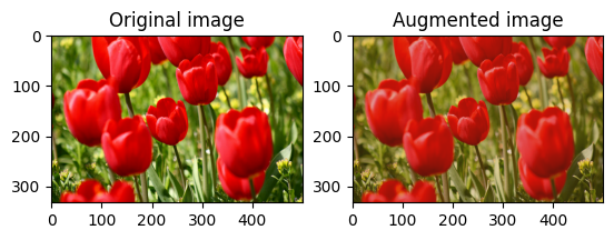
Randomly change image brightness
Randomly change the brightness of image using tf.image.stateless_random_brightness by providing a brightness factor and seed. The brightness factor is chosen randomly in the range [-max_delta, max_delta) and is associated with the given seed.
for i in range(3):
  seed = (i, 0)  # tuple of size (2,)
  stateless_random_brightness = tf.image.stateless_random_brightness(
      image, max_delta=0.95, seed=seed)
  visualize(image, stateless_random_brightness)
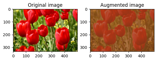
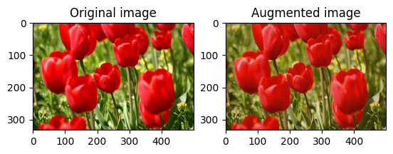
Randomly change image contrast
Randomly change the contrast of image using tf.image.stateless_random_contrast by providing a contrast range and seed. The contrast range is chosen randomly in the interval [lower, upper] and is associated with the given seed.
for i in range(3):
  seed = (i, 0)  # tuple of size (2,)
  stateless_random_contrast = tf.image.stateless_random_contrast(
      image, lower=0.1, upper=0.9, seed=seed)
  visualize(image, stateless_random_contrast)
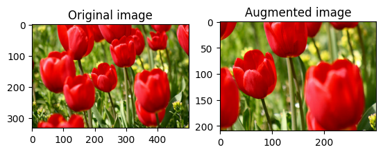
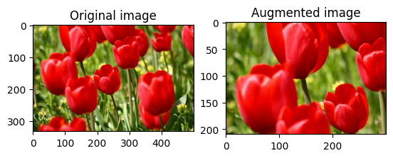
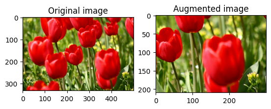
Randomly crop an image
Randomly crop image using tf.image.stateless_random_crop by providing target size and seed. The portion that gets cropped out of image is at a randomly chosen offset and is associated with the given seed.
for i in range(3):
  seed = (i, 0)  # tuple of size (2,)
  stateless_random_crop = tf.image.stateless_random_crop(
      image, size=[210, 300, 3], seed=seed)
  visualize(image, stateless_random_crop)
Apply augmentation to a dataset
Let's first download the image dataset again in case they are modified in the previous sections.
(train_datasets, val_ds, test_ds), metadata = tfds.load(
    'tf_flowers',
    split=['train[:80%]', 'train[80%:90%]', 'train[90%:]'],
    with_info=True,
    as_supervised=True,
)
Next, define a utility function for resizing and rescaling the images. This function will be used in unifying the size and scale of images in the dataset:
def resize_and_rescale(image, label):
  image = tf.cast(image, tf.float32)
  image = tf.image.resize(image, [IMG_SIZE, IMG_SIZE])
  image = (image / 255.0)
  return image, label
Let's also define the augment function that can apply the random transformations to the images. This function will be used on the dataset in the next step.
def augment(image_label, seed):
  image, label = image_label
  image, label = resize_and_rescale(image, label)
  image = tf.image.resize_with_crop_or_pad(image, IMG_SIZE + 6, IMG_SIZE + 6)
  # Make a new seed.
  new_seed = tf.random.split(seed, num=1)[0, :]
  # Random crop back to the original size.
  image = tf.image.stateless_random_crop(
      image, size=[IMG_SIZE, IMG_SIZE, 3], seed=seed)
  # Random brightness.
  image = tf.image.stateless_random_brightness(
      image, max_delta=0.5, seed=new_seed)
  image = tf.clip_by_value(image, 0, 1)
  return image, label
Option 1: Using tf.data.experimental.Counter
Create a tf.data.experimental.Counter object (let's call it counter) and Dataset.zip the dataset with (counter, counter). This will ensure that each image in the dataset gets associated with a unique value (of shape (2,)) based on counter which later can get passed into the augment function as the seed value for random transformations.
# Create a `Counter` object and `Dataset.zip` it together with the training set.
counter = tf.data.experimental.Counter()
train_ds = tf.data.Dataset.zip((train_datasets, (counter, counter)))
WARNING:tensorflow:From /tmpfs/tmp/ipykernel_85770/587852618.py:2: CounterV2 (from tensorflow.python.data.experimental.ops.counter) is deprecated and will be removed in a future version.
Instructions for updating:
Use `tf.data.Dataset.counter(...)` instead.
WARNING:tensorflow:From /tmpfs/tmp/ipykernel_85770/587852618.py:2: CounterV2 (from tensorflow.python.data.experimental.ops.counter) is deprecated and will be removed in a future version.
Instructions for updating:
Use `tf.data.Dataset.counter(...)` instead.
Map the augment function to the training dataset:
train_ds = (
    train_ds
    .shuffle(1000)
    .map(augment, num_parallel_calls=AUTOTUNE)
    .batch(batch_size)
    .prefetch(AUTOTUNE)
)
val_ds = (
    val_ds
    .map(resize_and_rescale, num_parallel_calls=AUTOTUNE)
    .batch(batch_size)
    .prefetch(AUTOTUNE)
)
test_ds = (
    test_ds
    .map(resize_and_rescale, num_parallel_calls=AUTOTUNE)
    .batch(batch_size)
    .prefetch(AUTOTUNE)
)
Option 2: Using tf.random.Generator
- Create a
tf.random.Generatorobject with an initialseedvalue. Calling themake_seedsfunction on the same generator object always returns a new, uniqueseedvalue. - Define a wrapper function that: 1) calls the
make_seedsfunction; and 2) passes the newly generatedseedvalue into theaugmentfunction for random transformations.
# Create a generator.
rng = tf.random.Generator.from_seed(123, alg='philox')
# Create a wrapper function for updating seeds.
def f(x, y):
  seed = rng.make_seeds(1)[:, 0]
  image, label = augment((x, y), seed)
  return image, label
Map the wrapper function f to the training dataset, and the resize_and_rescale function—to the validation and test sets:
train_ds = (
    train_datasets
    .shuffle(1000)
    .map(f, num_parallel_calls=AUTOTUNE)
    .batch(batch_size)
    .prefetch(AUTOTUNE)
)
val_ds = (
    val_ds
    .map(resize_and_rescale, num_parallel_calls=AUTOTUNE)
    .batch(batch_size)
    .prefetch(AUTOTUNE)
)
test_ds = (
    test_ds
    .map(resize_and_rescale, num_parallel_calls=AUTOTUNE)
    .batch(batch_size)
    .prefetch(AUTOTUNE)
)
These datasets can now be used to train a model as shown previously.
Next steps
This tutorial demonstrated data augmentation using Keras preprocessing layers and tf.image.
- To learn how to include preprocessing layers inside your model, refer to the Image classification tutorial.
- You may also be interested in learning how preprocessing layers can help you classify text, as shown in the Basic text classification tutorial.
- You can learn more about
tf.datain this guide, and you can learn how to configure your input pipelines for performance here.