
|
|
|
 View source on GitHub View source on GitHub
|
|
This tutorial shows how to load and preprocess an image dataset in three ways:
- First, you will use high-level Keras preprocessing utilities (such as
tf.keras.utils.image_dataset_from_directory) and layers (such astf.keras.layers.Rescaling) to read a directory of images on disk. - Next, you will write your own input pipeline from scratch using tf.data.
- Finally, you will download a dataset from the large catalog available in TensorFlow Datasets.
Setup
import numpy as np
import os
import PIL
import PIL.Image
import tensorflow as tf
import tensorflow_datasets as tfds
2024-08-16 07:35:28.601200: E external/local_xla/xla/stream_executor/cuda/cuda_fft.cc:485] Unable to register cuFFT factory: Attempting to register factory for plugin cuFFT when one has already been registered
2024-08-16 07:35:28.622447: E external/local_xla/xla/stream_executor/cuda/cuda_dnn.cc:8454] Unable to register cuDNN factory: Attempting to register factory for plugin cuDNN when one has already been registered
2024-08-16 07:35:28.628875: E external/local_xla/xla/stream_executor/cuda/cuda_blas.cc:1452] Unable to register cuBLAS factory: Attempting to register factory for plugin cuBLAS when one has already been registered
print(tf.__version__)
2.17.0
Download the flowers dataset
This tutorial uses a dataset of several thousand photos of flowers. The flowers dataset contains five sub-directories, one per class:
flowers_photos/
  daisy/
  dandelion/
  roses/
  sunflowers/
  tulips/
import pathlib
dataset_url = "https://storage.googleapis.com/download.tensorflow.org/example_images/flower_photos.tgz"
archive = tf.keras.utils.get_file(origin=dataset_url, extract=True)
data_dir = pathlib.Path(archive).with_suffix('')
Downloading data from https://storage.googleapis.com/download.tensorflow.org/example_images/flower_photos.tgz
228813984/228813984 ━━━━━━━━━━━━━━━━━━━━ 2s 0us/step
After downloading (218MB), you should now have a copy of the flower photos available. There are 3,670 total images:
image_count = len(list(data_dir.glob('*/*.jpg')))
print(image_count)
3670
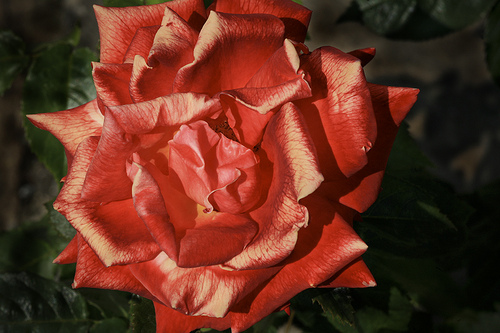
Each directory contains images of that type of flower. Here are some roses:
roses = list(data_dir.glob('roses/*'))
PIL.Image.open(str(roses[0]))

roses = list(data_dir.glob('roses/*'))
PIL.Image.open(str(roses[1]))
Load data using a Keras utility
Let's load these images off disk using the helpful tf.keras.utils.image_dataset_from_directory utility.
Create a dataset
Define some parameters for the loader:
batch_size = 32
img_height = 180
img_width = 180
It's good practice to use a validation split when developing your model. You will use 80% of the images for training and 20% for validation.
train_ds = tf.keras.utils.image_dataset_from_directory(
  data_dir,
  validation_split=0.2,
  subset="training",
  seed=123,
  image_size=(img_height, img_width),
  batch_size=batch_size)
Found 3670 files belonging to 5 classes.
Using 2936 files for training.
WARNING: All log messages before absl::InitializeLog() is called are written to STDERR
I0000 00:00:1723793736.323935  228334 cuda_executor.cc:1015] successful NUMA node read from SysFS had negative value (-1), but there must be at least one NUMA node, so returning NUMA node zero. See more at https://github.com/torvalds/linux/blob/v6.0/Documentation/ABI/testing/sysfs-bus-pci#L344-L355
I0000 00:00:1723793736.327688  228334 cuda_executor.cc:1015] successful NUMA node read from SysFS had negative value (-1), but there must be at least one NUMA node, so returning NUMA node zero. See more at https://github.com/torvalds/linux/blob/v6.0/Documentation/ABI/testing/sysfs-bus-pci#L344-L355
I0000 00:00:1723793736.331273  228334 cuda_executor.cc:1015] successful NUMA node read from SysFS had negative value (-1), but there must be at least one NUMA node, so returning NUMA node zero. See more at https://github.com/torvalds/linux/blob/v6.0/Documentation/ABI/testing/sysfs-bus-pci#L344-L355
I0000 00:00:1723793736.334862  228334 cuda_executor.cc:1015] successful NUMA node read from SysFS had negative value (-1), but there must be at least one NUMA node, so returning NUMA node zero. See more at https://github.com/torvalds/linux/blob/v6.0/Documentation/ABI/testing/sysfs-bus-pci#L344-L355
I0000 00:00:1723793736.346577  228334 cuda_executor.cc:1015] successful NUMA node read from SysFS had negative value (-1), but there must be at least one NUMA node, so returning NUMA node zero. See more at https://github.com/torvalds/linux/blob/v6.0/Documentation/ABI/testing/sysfs-bus-pci#L344-L355
I0000 00:00:1723793736.350078  228334 cuda_executor.cc:1015] successful NUMA node read from SysFS had negative value (-1), but there must be at least one NUMA node, so returning NUMA node zero. See more at https://github.com/torvalds/linux/blob/v6.0/Documentation/ABI/testing/sysfs-bus-pci#L344-L355
I0000 00:00:1723793736.353446  228334 cuda_executor.cc:1015] successful NUMA node read from SysFS had negative value (-1), but there must be at least one NUMA node, so returning NUMA node zero. See more at https://github.com/torvalds/linux/blob/v6.0/Documentation/ABI/testing/sysfs-bus-pci#L344-L355
I0000 00:00:1723793736.356758  228334 cuda_executor.cc:1015] successful NUMA node read from SysFS had negative value (-1), but there must be at least one NUMA node, so returning NUMA node zero. See more at https://github.com/torvalds/linux/blob/v6.0/Documentation/ABI/testing/sysfs-bus-pci#L344-L355
I0000 00:00:1723793736.360253  228334 cuda_executor.cc:1015] successful NUMA node read from SysFS had negative value (-1), but there must be at least one NUMA node, so returning NUMA node zero. See more at https://github.com/torvalds/linux/blob/v6.0/Documentation/ABI/testing/sysfs-bus-pci#L344-L355
I0000 00:00:1723793736.363838  228334 cuda_executor.cc:1015] successful NUMA node read from SysFS had negative value (-1), but there must be at least one NUMA node, so returning NUMA node zero. See more at https://github.com/torvalds/linux/blob/v6.0/Documentation/ABI/testing/sysfs-bus-pci#L344-L355
I0000 00:00:1723793736.367268  228334 cuda_executor.cc:1015] successful NUMA node read from SysFS had negative value (-1), but there must be at least one NUMA node, so returning NUMA node zero. See more at https://github.com/torvalds/linux/blob/v6.0/Documentation/ABI/testing/sysfs-bus-pci#L344-L355
I0000 00:00:1723793736.370622  228334 cuda_executor.cc:1015] successful NUMA node read from SysFS had negative value (-1), but there must be at least one NUMA node, so returning NUMA node zero. See more at https://github.com/torvalds/linux/blob/v6.0/Documentation/ABI/testing/sysfs-bus-pci#L344-L355
I0000 00:00:1723793737.615909  228334 cuda_executor.cc:1015] successful NUMA node read from SysFS had negative value (-1), but there must be at least one NUMA node, so returning NUMA node zero. See more at https://github.com/torvalds/linux/blob/v6.0/Documentation/ABI/testing/sysfs-bus-pci#L344-L355
I0000 00:00:1723793737.618086  228334 cuda_executor.cc:1015] successful NUMA node read from SysFS had negative value (-1), but there must be at least one NUMA node, so returning NUMA node zero. See more at https://github.com/torvalds/linux/blob/v6.0/Documentation/ABI/testing/sysfs-bus-pci#L344-L355
I0000 00:00:1723793737.620163  228334 cuda_executor.cc:1015] successful NUMA node read from SysFS had negative value (-1), but there must be at least one NUMA node, so returning NUMA node zero. See more at https://github.com/torvalds/linux/blob/v6.0/Documentation/ABI/testing/sysfs-bus-pci#L344-L355
I0000 00:00:1723793737.622223  228334 cuda_executor.cc:1015] successful NUMA node read from SysFS had negative value (-1), but there must be at least one NUMA node, so returning NUMA node zero. See more at https://github.com/torvalds/linux/blob/v6.0/Documentation/ABI/testing/sysfs-bus-pci#L344-L355
I0000 00:00:1723793737.624312  228334 cuda_executor.cc:1015] successful NUMA node read from SysFS had negative value (-1), but there must be at least one NUMA node, so returning NUMA node zero. See more at https://github.com/torvalds/linux/blob/v6.0/Documentation/ABI/testing/sysfs-bus-pci#L344-L355
I0000 00:00:1723793737.626332  228334 cuda_executor.cc:1015] successful NUMA node read from SysFS had negative value (-1), but there must be at least one NUMA node, so returning NUMA node zero. See more at https://github.com/torvalds/linux/blob/v6.0/Documentation/ABI/testing/sysfs-bus-pci#L344-L355
I0000 00:00:1723793737.628286  228334 cuda_executor.cc:1015] successful NUMA node read from SysFS had negative value (-1), but there must be at least one NUMA node, so returning NUMA node zero. See more at https://github.com/torvalds/linux/blob/v6.0/Documentation/ABI/testing/sysfs-bus-pci#L344-L355
I0000 00:00:1723793737.630249  228334 cuda_executor.cc:1015] successful NUMA node read from SysFS had negative value (-1), but there must be at least one NUMA node, so returning NUMA node zero. See more at https://github.com/torvalds/linux/blob/v6.0/Documentation/ABI/testing/sysfs-bus-pci#L344-L355
I0000 00:00:1723793737.632230  228334 cuda_executor.cc:1015] successful NUMA node read from SysFS had negative value (-1), but there must be at least one NUMA node, so returning NUMA node zero. See more at https://github.com/torvalds/linux/blob/v6.0/Documentation/ABI/testing/sysfs-bus-pci#L344-L355
I0000 00:00:1723793737.634261  228334 cuda_executor.cc:1015] successful NUMA node read from SysFS had negative value (-1), but there must be at least one NUMA node, so returning NUMA node zero. See more at https://github.com/torvalds/linux/blob/v6.0/Documentation/ABI/testing/sysfs-bus-pci#L344-L355
I0000 00:00:1723793737.636226  228334 cuda_executor.cc:1015] successful NUMA node read from SysFS had negative value (-1), but there must be at least one NUMA node, so returning NUMA node zero. See more at https://github.com/torvalds/linux/blob/v6.0/Documentation/ABI/testing/sysfs-bus-pci#L344-L355
I0000 00:00:1723793737.638171  228334 cuda_executor.cc:1015] successful NUMA node read from SysFS had negative value (-1), but there must be at least one NUMA node, so returning NUMA node zero. See more at https://github.com/torvalds/linux/blob/v6.0/Documentation/ABI/testing/sysfs-bus-pci#L344-L355
I0000 00:00:1723793737.677165  228334 cuda_executor.cc:1015] successful NUMA node read from SysFS had negative value (-1), but there must be at least one NUMA node, so returning NUMA node zero. See more at https://github.com/torvalds/linux/blob/v6.0/Documentation/ABI/testing/sysfs-bus-pci#L344-L355
I0000 00:00:1723793737.679297  228334 cuda_executor.cc:1015] successful NUMA node read from SysFS had negative value (-1), but there must be at least one NUMA node, so returning NUMA node zero. See more at https://github.com/torvalds/linux/blob/v6.0/Documentation/ABI/testing/sysfs-bus-pci#L344-L355
I0000 00:00:1723793737.681295  228334 cuda_executor.cc:1015] successful NUMA node read from SysFS had negative value (-1), but there must be at least one NUMA node, so returning NUMA node zero. See more at https://github.com/torvalds/linux/blob/v6.0/Documentation/ABI/testing/sysfs-bus-pci#L344-L355
I0000 00:00:1723793737.683291  228334 cuda_executor.cc:1015] successful NUMA node read from SysFS had negative value (-1), but there must be at least one NUMA node, so returning NUMA node zero. See more at https://github.com/torvalds/linux/blob/v6.0/Documentation/ABI/testing/sysfs-bus-pci#L344-L355
I0000 00:00:1723793737.685306  228334 cuda_executor.cc:1015] successful NUMA node read from SysFS had negative value (-1), but there must be at least one NUMA node, so returning NUMA node zero. See more at https://github.com/torvalds/linux/blob/v6.0/Documentation/ABI/testing/sysfs-bus-pci#L344-L355
I0000 00:00:1723793737.687341  228334 cuda_executor.cc:1015] successful NUMA node read from SysFS had negative value (-1), but there must be at least one NUMA node, so returning NUMA node zero. See more at https://github.com/torvalds/linux/blob/v6.0/Documentation/ABI/testing/sysfs-bus-pci#L344-L355
I0000 00:00:1723793737.689297  228334 cuda_executor.cc:1015] successful NUMA node read from SysFS had negative value (-1), but there must be at least one NUMA node, so returning NUMA node zero. See more at https://github.com/torvalds/linux/blob/v6.0/Documentation/ABI/testing/sysfs-bus-pci#L344-L355
I0000 00:00:1723793737.691269  228334 cuda_executor.cc:1015] successful NUMA node read from SysFS had negative value (-1), but there must be at least one NUMA node, so returning NUMA node zero. See more at https://github.com/torvalds/linux/blob/v6.0/Documentation/ABI/testing/sysfs-bus-pci#L344-L355
I0000 00:00:1723793737.693297  228334 cuda_executor.cc:1015] successful NUMA node read from SysFS had negative value (-1), but there must be at least one NUMA node, so returning NUMA node zero. See more at https://github.com/torvalds/linux/blob/v6.0/Documentation/ABI/testing/sysfs-bus-pci#L344-L355
I0000 00:00:1723793737.695724  228334 cuda_executor.cc:1015] successful NUMA node read from SysFS had negative value (-1), but there must be at least one NUMA node, so returning NUMA node zero. See more at https://github.com/torvalds/linux/blob/v6.0/Documentation/ABI/testing/sysfs-bus-pci#L344-L355
I0000 00:00:1723793737.698128  228334 cuda_executor.cc:1015] successful NUMA node read from SysFS had negative value (-1), but there must be at least one NUMA node, so returning NUMA node zero. See more at https://github.com/torvalds/linux/blob/v6.0/Documentation/ABI/testing/sysfs-bus-pci#L344-L355
I0000 00:00:1723793737.700565  228334 cuda_executor.cc:1015] successful NUMA node read from SysFS had negative value (-1), but there must be at least one NUMA node, so returning NUMA node zero. See more at https://github.com/torvalds/linux/blob/v6.0/Documentation/ABI/testing/sysfs-bus-pci#L344-L355
val_ds = tf.keras.utils.image_dataset_from_directory(
  data_dir,
  validation_split=0.2,
  subset="validation",
  seed=123,
  image_size=(img_height, img_width),
  batch_size=batch_size)
Found 3670 files belonging to 5 classes.
Using 734 files for validation.
You can find the class names in the class_names attribute on these datasets.
class_names = train_ds.class_names
print(class_names)
['daisy', 'dandelion', 'roses', 'sunflowers', 'tulips']
Visualize the data
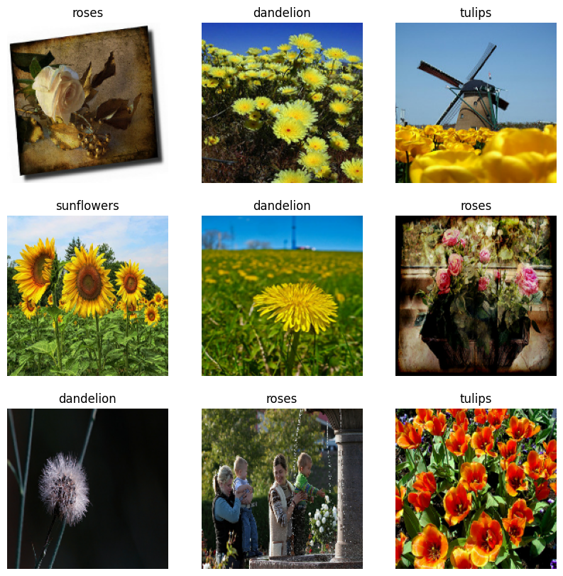
Here are the first nine images from the training dataset.
import matplotlib.pyplot as plt

plt.figure(figsize=(10, 10))
for images, labels in train_ds.take(1):
  for i in range(9):
    ax = plt.subplot(3, 3, i + 1)
    plt.imshow(images[i].numpy().astype("uint8"))
    plt.title(class_names[labels[i]])
    plt.axis("off")
You can train a model using these datasets by passing them to model.fit (shown later in this tutorial). If you like, you can also manually iterate over the dataset and retrieve batches of images:
for image_batch, labels_batch in train_ds:
  print(image_batch.shape)
  print(labels_batch.shape)
  break
(32, 180, 180, 3)
(32,)
The image_batch is a tensor of the shape (32, 180, 180, 3). This is a batch of 32 images of shape 180x180x3 (the last dimension refers to color channels RGB). The label_batch is a tensor of the shape (32,), these are corresponding labels to the 32 images.
You can call .numpy() on either of these tensors to convert them to a numpy.ndarray.
Standardize the data
The RGB channel values are in the [0, 255] range. This is not ideal for a neural network; in general you should seek to make your input values small.
Here, you will standardize values to be in the [0, 1] range by using tf.keras.layers.Rescaling:
normalization_layer = tf.keras.layers.Rescaling(1./255)
There are two ways to use this layer. You can apply it to the dataset by calling Dataset.map:
normalized_ds = train_ds.map(lambda x, y: (normalization_layer(x), y))
image_batch, labels_batch = next(iter(normalized_ds))
first_image = image_batch[0]
# Notice the pixel values are now in `[0,1]`.
print(np.min(first_image), np.max(first_image))
0.0 0.96902645
Or, you can include the layer inside your model definition to simplify deployment. You will use the second approach here.
Configure the dataset for performance
Let's make sure to use buffered prefetching so you can yield data from disk without having I/O become blocking. These are two important methods you should use when loading data:
Dataset.cachekeeps the images in memory after they're loaded off disk during the first epoch. This will ensure the dataset does not become a bottleneck while training your model. If your dataset is too large to fit into memory, you can also use this method to create a performant on-disk cache.Dataset.prefetchoverlaps data preprocessing and model execution while training.
Interested readers can learn more about both methods, as well as how to cache data to disk in the Prefetching section of the Better performance with the tf.data API guide.
AUTOTUNE = tf.data.AUTOTUNE

train_ds = train_ds.cache().prefetch(buffer_size=AUTOTUNE)
val_ds = val_ds.cache().prefetch(buffer_size=AUTOTUNE)
Train a model
For completeness, you will show how to train a simple model using the datasets you have just prepared.
The Sequential model consists of three convolution blocks (tf.keras.layers.Conv2D) with a max pooling layer (tf.keras.layers.MaxPooling2D) in each of them. There's a fully-connected layer (tf.keras.layers.Dense) with 128 units on top of it that is activated by a ReLU activation function ('relu'). This model has not been tuned in any way—the goal is to show you the mechanics using the datasets you just created. To learn more about image classification, visit the Image classification tutorial.
num_classes = 5

model = tf.keras.Sequential([
  tf.keras.layers.Rescaling(1./255),
  tf.keras.layers.Conv2D(32, 3, activation='relu'),
  tf.keras.layers.MaxPooling2D(),
  tf.keras.layers.Conv2D(32, 3, activation='relu'),
  tf.keras.layers.MaxPooling2D(),
  tf.keras.layers.Conv2D(32, 3, activation='relu'),
  tf.keras.layers.MaxPooling2D(),
  tf.keras.layers.Flatten(),
  tf.keras.layers.Dense(128, activation='relu'),
  tf.keras.layers.Dense(num_classes)
])
Choose the tf.keras.optimizers.Adam optimizer and tf.keras.losses.SparseCategoricalCrossentropy loss function. To view training and validation accuracy for each training epoch, pass the metrics argument to Model.compile.
model.compile(
  optimizer='adam',
  loss=tf.keras.losses.SparseCategoricalCrossentropy(from_logits=True),
  metrics=['accuracy'])
model.fit(
  train_ds,
  validation_data=val_ds,
  epochs=3
)
Epoch 1/3
WARNING: All log messages before absl::InitializeLog() is called are written to STDERR
I0000 00:00:1723793742.229752  228538 service.cc:146] XLA service 0x7f8424005180 initialized for platform CUDA (this does not guarantee that XLA will be used). Devices:
I0000 00:00:1723793742.229788  228538 service.cc:154]   StreamExecutor device (0): Tesla T4, Compute Capability 7.5
I0000 00:00:1723793742.229793  228538 service.cc:154]   StreamExecutor device (1): Tesla T4, Compute Capability 7.5
I0000 00:00:1723793742.229796  228538 service.cc:154]   StreamExecutor device (2): Tesla T4, Compute Capability 7.5
I0000 00:00:1723793742.229799  228538 service.cc:154]   StreamExecutor device (3): Tesla T4, Compute Capability 7.5
E0000 00:00:1723793743.747934  228538 gpu_timer.cc:183] Delay kernel timed out: measured time has sub-optimal accuracy. There may be a missing warmup execution, please investigate in Nsight Systems.
E0000 00:00:1723793743.889619  228538 gpu_timer.cc:183] Delay kernel timed out: measured time has sub-optimal accuracy. There may be a missing warmup execution, please investigate in Nsight Systems.
10/92 ━━━━━━━━━━━━━━━━━━━━ 1s 19ms/step - accuracy: 0.2397 - loss: 1.6561
I0000 00:00:1723793745.306928  228538 device_compiler.h:188] Compiled cluster using XLA!  This line is logged at most once for the lifetime of the process.
91/92 ━━━━━━━━━━━━━━━━━━━━ 0s 31ms/step - accuracy: 0.3728 - loss: 1.4181
E0000 00:00:1723793748.938167  228536 gpu_timer.cc:183] Delay kernel timed out: measured time has sub-optimal accuracy. There may be a missing warmup execution, please investigate in Nsight Systems.
E0000 00:00:1723793749.078774  228536 gpu_timer.cc:183] Delay kernel timed out: measured time has sub-optimal accuracy. There may be a missing warmup execution, please investigate in Nsight Systems.
92/92 ━━━━━━━━━━━━━━━━━━━━ 12s 79ms/step - accuracy: 0.3744 - loss: 1.4152 - val_accuracy: 0.5463 - val_loss: 1.1106
Epoch 2/3
92/92 ━━━━━━━━━━━━━━━━━━━━ 2s 20ms/step - accuracy: 0.5915 - loss: 1.0141 - val_accuracy: 0.5763 - val_loss: 1.0378
Epoch 3/3
92/92 ━━━━━━━━━━━━━━━━━━━━ 2s 20ms/step - accuracy: 0.6581 - loss: 0.8870 - val_accuracy: 0.6090 - val_loss: 0.9559
<keras.src.callbacks.history.History at 0x7f8584228c40>
You may notice the validation accuracy is low compared to the training accuracy, indicating your model is overfitting. You can learn more about overfitting and how to reduce it in this tutorial.
Using tf.data for finer control
The above Keras preprocessing utility—tf.keras.utils.image_dataset_from_directory—is a convenient way to create a tf.data.Dataset from a directory of images.
For finer grain control, you can write your own input pipeline using tf.data. This section shows how to do just that, beginning with the file paths from the TGZ file you downloaded earlier.
list_ds = tf.data.Dataset.list_files(str(data_dir/'*/*'), shuffle=False)
list_ds = list_ds.shuffle(image_count, reshuffle_each_iteration=False)
for f in list_ds.take(5):
  print(f.numpy())
b'/home/kbuilder/.keras/datasets/flower_photos/dandelion/16237158409_01913cf918_n.jpg'
b'/home/kbuilder/.keras/datasets/flower_photos/dandelion/4654848357_9549351e0b_n.jpg'
b'/home/kbuilder/.keras/datasets/flower_photos/dandelion/19443726008_8c9c68efa7_m.jpg'
b'/home/kbuilder/.keras/datasets/flower_photos/tulips/16751015081_af2ef77c9a_n.jpg'
b'/home/kbuilder/.keras/datasets/flower_photos/dandelion/2330343016_23acc484ee.jpg'
The tree structure of the files can be used to compile a class_names list.
class_names = np.array(sorted([item.name for item in data_dir.glob('*') if item.name != "LICENSE.txt"]))
print(class_names)
['daisy' 'dandelion' 'roses' 'sunflowers' 'tulips']
Split the dataset into training and validation sets:
val_size = int(image_count * 0.2)
train_ds = list_ds.skip(val_size)
val_ds = list_ds.take(val_size)
You can print the length of each dataset as follows:
print(tf.data.experimental.cardinality(train_ds).numpy())
print(tf.data.experimental.cardinality(val_ds).numpy())
2936
734
Write a short function that converts a file path to an (img, label) pair:
def get_label(file_path):
  # Convert the path to a list of path components
  parts = tf.strings.split(file_path, os.path.sep)
  # The second to last is the class-directory
  one_hot = parts[-2] == class_names
  # Integer encode the label
  return tf.argmax(one_hot)
def decode_img(img):
  # Convert the compressed string to a 3D uint8 tensor
  img = tf.io.decode_jpeg(img, channels=3)
  # Resize the image to the desired size
  return tf.image.resize(img, [img_height, img_width])
def process_path(file_path):
  label = get_label(file_path)
  # Load the raw data from the file as a string
  img = tf.io.read_file(file_path)
  img = decode_img(img)
  return img, label
Use Dataset.map to create a dataset of image, label pairs:
# Set `num_parallel_calls` so multiple images are loaded/processed in parallel.
train_ds = train_ds.map(process_path, num_parallel_calls=AUTOTUNE)
val_ds = val_ds.map(process_path, num_parallel_calls=AUTOTUNE)
for image, label in train_ds.take(1):
  print("Image shape: ", image.numpy().shape)
  print("Label: ", label.numpy())
Image shape:  (180, 180, 3)
Label:  4
Configure dataset for performance
To train a model with this dataset you will want the data:
- To be well shuffled.
- To be batched.
- Batches to be available as soon as possible.
These features can be added using the tf.data API. For more details, visit the Input Pipeline Performance guide.
def configure_for_performance(ds):
  ds = ds.cache()
  ds = ds.shuffle(buffer_size=1000)
  ds = ds.batch(batch_size)
  ds = ds.prefetch(buffer_size=AUTOTUNE)
  return ds

train_ds = configure_for_performance(train_ds)
val_ds = configure_for_performance(val_ds)
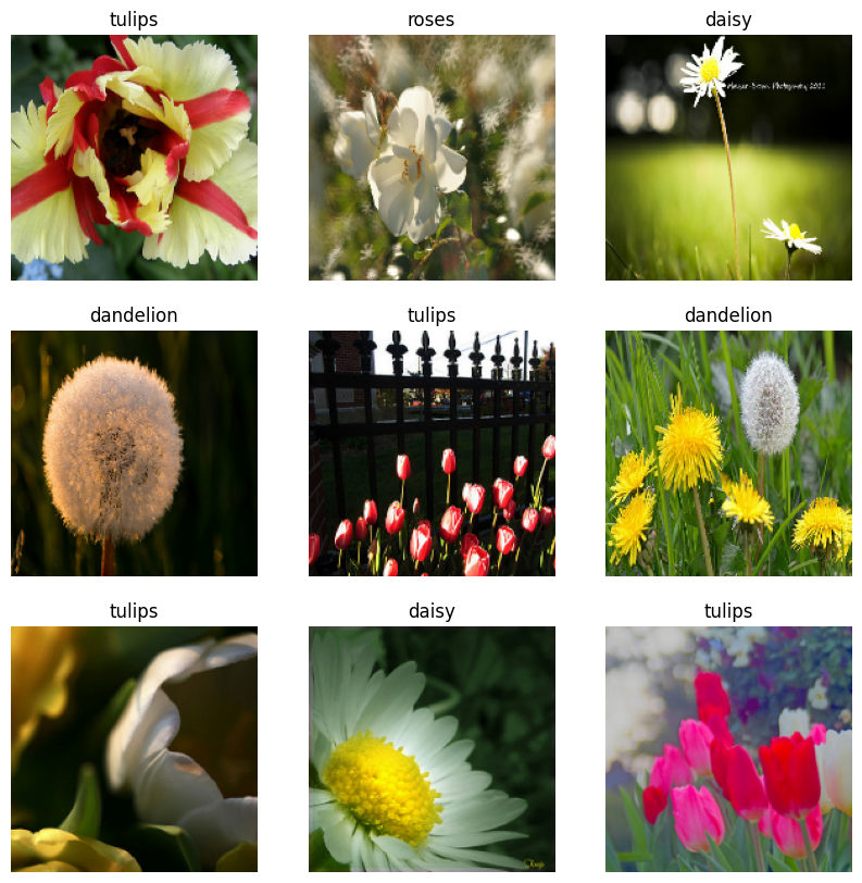
Visualize the data
You can visualize this dataset similarly to the one you created previously:
image_batch, label_batch = next(iter(train_ds))

plt.figure(figsize=(10, 10))
for i in range(9):
  ax = plt.subplot(3, 3, i + 1)
  plt.imshow(image_batch[i].numpy().astype("uint8"))
  label = label_batch[i]
  plt.title(class_names[label])
  plt.axis("off")
2024-08-16 07:35:56.791290: W tensorflow/core/kernels/data/cache_dataset_ops.cc:913] The calling iterator did not fully read the dataset being cached. In order to avoid unexpected truncation of the dataset, the partially cached contents of the dataset will be discarded. This can happen if you have an input pipeline similar to `dataset.cache().take(k).repeat()`. You should use `dataset.take(k).cache().repeat()` instead.
Continue training the model
You have now manually built a similar tf.data.Dataset to the one created by tf.keras.utils.image_dataset_from_directory above. You can continue training the model with it. As before, you will train for just a few epochs to keep the running time short.
model.fit(
  train_ds,
  validation_data=val_ds,
  epochs=3
)
Epoch 1/3
92/92 ━━━━━━━━━━━━━━━━━━━━ 6s 48ms/step - accuracy: 0.7026 - loss: 0.7613 - val_accuracy: 0.7057 - val_loss: 0.7631
Epoch 2/3
92/92 ━━━━━━━━━━━━━━━━━━━━ 2s 24ms/step - accuracy: 0.7659 - loss: 0.6259 - val_accuracy: 0.7139 - val_loss: 0.7349
Epoch 3/3
92/92 ━━━━━━━━━━━━━━━━━━━━ 2s 23ms/step - accuracy: 0.8536 - loss: 0.4182 - val_accuracy: 0.7330 - val_loss: 0.7181
<keras.src.callbacks.history.History at 0x7f85641dbf40>
Using TensorFlow Datasets
So far, this tutorial has focused on loading data off disk. You can also find a dataset to use by exploring the large catalog of easy-to-download datasets at TensorFlow Datasets.
As you have previously loaded the Flowers dataset off disk, let's now import it with TensorFlow Datasets.
Download the Flowers dataset using TensorFlow Datasets:
(train_ds, val_ds, test_ds), metadata = tfds.load(
    'tf_flowers',
    split=['train[:80%]', 'train[80%:90%]', 'train[90%:]'],
    with_info=True,
    as_supervised=True,
)
The flowers dataset has five classes:
num_classes = metadata.features['label'].num_classes
print(num_classes)
5
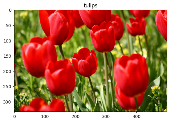
Retrieve an image from the dataset:
get_label_name = metadata.features['label'].int2str

image, label = next(iter(train_ds))
_ = plt.imshow(image)
_ = plt.title(get_label_name(label))
2024-08-16 07:36:09.400520: W tensorflow/core/kernels/data/cache_dataset_ops.cc:913] The calling iterator did not fully read the dataset being cached. In order to avoid unexpected truncation of the dataset, the partially cached contents of the dataset will be discarded. This can happen if you have an input pipeline similar to `dataset.cache().take(k).repeat()`. You should use `dataset.take(k).cache().repeat()` instead.
As before, remember to batch, shuffle, and configure the training, validation, and test sets for performance:
train_ds = configure_for_performance(train_ds)
val_ds = configure_for_performance(val_ds)
test_ds = configure_for_performance(test_ds)
You can find a complete example of working with the Flowers dataset and TensorFlow Datasets by visiting the Data augmentation tutorial.
Next steps
This tutorial showed two ways of loading images off disk. First, you learned how to load and preprocess an image dataset using Keras preprocessing layers and utilities. Next, you learned how to write an input pipeline from scratch using tf.data. Finally, you learned how to download a dataset from TensorFlow Datasets.
For your next steps:
- You can learn how to add data augmentation.
- To learn more about
tf.data, you can visit the tf.data: Build TensorFlow input pipelines guide.