
|
|
|
 View source on GitHub View source on GitHub
|
|
This tutorial demonstrates how to classify a highly imbalanced dataset in which the number of examples in one class greatly outnumbers the examples in another. You will work with the Credit Card Fraud Detection dataset hosted on Kaggle. The aim is to detect a mere 492 fraudulent transactions from 284,807 transactions in total. You will use Keras to define the model and class weights to help the model learn from the imbalanced data. .
This tutorial contains complete code to:
- Load a CSV file using Pandas.
- Create train, validation, and test sets.
- Define and train a model using Keras (including setting class weights).
- Evaluate the model using various metrics (including precision and recall).
- Select a threshold for a probabilistic classifier to get a deterministic classifier.
- Try and compare with class weighted modelling and oversampling.
Setup
import tensorflow as tf
from tensorflow import keras

import os
import tempfile

import matplotlib as mpl
import matplotlib.pyplot as plt
import numpy as np
import pandas as pd
import seaborn as sns

import sklearn
from sklearn.metrics import confusion_matrix
from sklearn.model_selection import train_test_split
from sklearn.preprocessing import StandardScaler
2024-08-20 01:23:52.305388: E external/local_xla/xla/stream_executor/cuda/cuda_fft.cc:485] Unable to register cuFFT factory: Attempting to register factory for plugin cuFFT when one has already been registered
2024-08-20 01:23:52.326935: E external/local_xla/xla/stream_executor/cuda/cuda_dnn.cc:8454] Unable to register cuDNN factory: Attempting to register factory for plugin cuDNN when one has already been registered
2024-08-20 01:23:52.333533: E external/local_xla/xla/stream_executor/cuda/cuda_blas.cc:1452] Unable to register cuBLAS factory: Attempting to register factory for plugin cuBLAS when one has already been registered
mpl.rcParams['figure.figsize'] = (12, 10)
colors = plt.rcParams['axes.prop_cycle'].by_key()['color']
Data processing and exploration
Download the Kaggle Credit Card Fraud data set
Pandas is a Python library with many helpful utilities for loading and working with structured data. It can be used to download CSVs into a Pandas DataFrame.
file = tf.keras.utils
raw_df = pd.read_csv('https://storage.googleapis.com/download.tensorflow.org/data/creditcard.csv')
raw_df.head()
raw_df[['Time', 'V1', 'V2', 'V3', 'V4', 'V5', 'V26', 'V27', 'V28', 'Amount', 'Class']].describe()
Examine the class label imbalance
Let's look at the dataset imbalance:
neg, pos = np.bincount(raw_df['Class'])
total = neg + pos
print('Examples:\n    Total: {}\n    Positive: {} ({:.2f}% of total)\n'.format(
    total, pos, 100 * pos / total))
Examples:
    Total: 284807
    Positive: 492 (0.17% of total)
This shows the small fraction of positive samples.
Clean, split and normalize the data
The raw data has a few issues. First the Time and Amount columns are too variable to use directly. Drop the Time column (since it's not clear what it means) and take the log of the Amount column to reduce its range.
cleaned_df = raw_df.copy()

# You don't want the `Time` column.
cleaned_df.pop('Time')

# The `Amount` column covers a huge range. Convert to log-space.
eps = 0.001 # 0 => 0.1¢
cleaned_df['Log Amount'] = np.log(cleaned_df.pop('Amount')+eps)
Split the dataset into train, validation, and test sets. The validation set is used during the model fitting to evaluate the loss and any metrics, however the model is not fit with this data. The test set is completely unused during the training phase and is only used at the end to evaluate how well the model generalizes to new data. This is especially important with imbalanced datasets where overfitting is a significant concern from the lack of training data.
# Use a utility from sklearn to split and shuffle your dataset.
train_df, test_df = train_test_split(cleaned_df, test_size=0.2)
train_df, val_df = train_test_split(train_df, test_size=0.2)

# Form np arrays of labels and features.
train_labels = np.array(train_df.pop('Class')).reshape(-1, 1)
bool_train_labels = train_labels[:, 0] != 0
val_labels = np.array(val_df.pop('Class')).reshape(-1, 1)
test_labels = np.array(test_df.pop('Class')).reshape(-1, 1)

train_features = np.array(train_df)
val_features = np.array(val_df)
test_features = np.array(test_df)
We check whether the distribution of the classes in the three sets is about the same or not.
print(f'Average class probability in training set:   {train_labels.mean():.4f}')
print(f'Average class probability in validation set: {val_labels.mean():.4f}')
print(f'Average class probability in test set:       {test_labels.mean():.4f}')
Average class probability in training set:   0.0017
Average class probability in validation set: 0.0018
Average class probability in test set:       0.0018
Given the small number of positive labels, this seems about right.
Normalize the input features using the sklearn StandardScaler. This will set the mean to 0 and standard deviation to 1.
scaler = StandardScaler()
train_features = scaler.fit_transform(train_features)

val_features = scaler.transform(val_features)
test_features = scaler.transform(test_features)

train_features = np.clip(train_features, -5, 5)
val_features = np.clip(val_features, -5, 5)
test_features = np.clip(test_features, -5, 5)


print('Training labels shape:', train_labels.shape)
print('Validation labels shape:', val_labels.shape)
print('Test labels shape:', test_labels.shape)

print('Training features shape:', train_features.shape)
print('Validation features shape:', val_features.shape)
print('Test features shape:', test_features.shape)
Training labels shape: (182276, 1)
Validation labels shape: (45569, 1)
Test labels shape: (56962, 1)
Training features shape: (182276, 29)
Validation features shape: (45569, 29)
Test features shape: (56962, 29)
Look at the data distribution
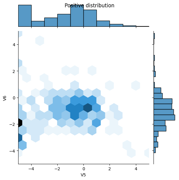
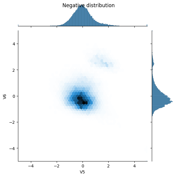
Next compare the distributions of the positive and negative examples over a few features. Good questions to ask yourself at this point are:
- Do these distributions make sense?
- Yes. You've normalized the input and these are mostly concentrated in the
+/- 2range.
- Yes. You've normalized the input and these are mostly concentrated in the
- Can you see the difference between the distributions?
- Yes the positive examples contain a much higher rate of extreme values.
pos_df = pd.DataFrame(train_features[ bool_train_labels], columns=train_df.columns)
neg_df = pd.DataFrame(train_features[~bool_train_labels], columns=train_df.columns)

sns.jointplot(x=pos_df['V5'], y=pos_df['V6'],
              kind='hex', xlim=(-5,5), ylim=(-5,5))
plt.suptitle("Positive distribution")

sns.jointplot(x=neg_df['V5'], y=neg_df['V6'],
              kind='hex', xlim=(-5,5), ylim=(-5,5))
_ = plt.suptitle("Negative distribution")
Define the model and metrics
Define a function that creates a simple neural network with a densly connected hidden layer, a dropout layer to reduce overfitting, and an output sigmoid layer that returns the probability of a transaction being fraudulent:
METRICS = [
      keras.metrics.BinaryCrossentropy(name='cross entropy'),  # same as model's loss
      keras.metrics.MeanSquaredError(name='Brier score'),
      keras.metrics.TruePositives(name='tp'),
      keras.metrics.FalsePositives(name='fp'),
      keras.metrics.TrueNegatives(name='tn'),
      keras.metrics.FalseNegatives(name='fn'),
      keras.metrics.BinaryAccuracy(name='accuracy'),
      keras.metrics.Precision(name='precision'),
      keras.metrics.Recall(name='recall'),
      keras.metrics.AUC(name='auc'),
      keras.metrics.AUC(name='prc', curve='PR'), # precision-recall curve
]

def make_model(metrics=METRICS, output_bias=None):
  if output_bias is not None:
    output_bias = tf.keras.initializers.Constant(output_bias)
  model = keras.Sequential([
      keras.layers.Dense(
          16, activation='relu',
          input_shape=(train_features.shape[-1],)),
      keras.layers.Dropout(0.5),
      keras.layers.Dense(1, activation='sigmoid',
                         bias_initializer=output_bias),
  ])

  model.compile(
      optimizer=keras.optimizers.Adam(learning_rate=1e-3),
      loss=keras.losses.BinaryCrossentropy(),
      metrics=metrics)

  return model
WARNING: All log messages before absl::InitializeLog() is called are written to STDERR
I0000 00:00:1724117041.170464    9349 cuda_executor.cc:1015] successful NUMA node read from SysFS had negative value (-1), but there must be at least one NUMA node, so returning NUMA node zero. See more at https://github.com/torvalds/linux/blob/v6.0/Documentation/ABI/testing/sysfs-bus-pci#L344-L355
I0000 00:00:1724117041.173954    9349 cuda_executor.cc:1015] successful NUMA node read from SysFS had negative value (-1), but there must be at least one NUMA node, so returning NUMA node zero. See more at https://github.com/torvalds/linux/blob/v6.0/Documentation/ABI/testing/sysfs-bus-pci#L344-L355
I0000 00:00:1724117041.177520    9349 cuda_executor.cc:1015] successful NUMA node read from SysFS had negative value (-1), but there must be at least one NUMA node, so returning NUMA node zero. See more at https://github.com/torvalds/linux/blob/v6.0/Documentation/ABI/testing/sysfs-bus-pci#L344-L355
I0000 00:00:1724117041.181109    9349 cuda_executor.cc:1015] successful NUMA node read from SysFS had negative value (-1), but there must be at least one NUMA node, so returning NUMA node zero. See more at https://github.com/torvalds/linux/blob/v6.0/Documentation/ABI/testing/sysfs-bus-pci#L344-L355
I0000 00:00:1724117041.192229    9349 cuda_executor.cc:1015] successful NUMA node read from SysFS had negative value (-1), but there must be at least one NUMA node, so returning NUMA node zero. See more at https://github.com/torvalds/linux/blob/v6.0/Documentation/ABI/testing/sysfs-bus-pci#L344-L355
I0000 00:00:1724117041.195501    9349 cuda_executor.cc:1015] successful NUMA node read from SysFS had negative value (-1), but there must be at least one NUMA node, so returning NUMA node zero. See more at https://github.com/torvalds/linux/blob/v6.0/Documentation/ABI/testing/sysfs-bus-pci#L344-L355
I0000 00:00:1724117041.198855    9349 cuda_executor.cc:1015] successful NUMA node read from SysFS had negative value (-1), but there must be at least one NUMA node, so returning NUMA node zero. See more at https://github.com/torvalds/linux/blob/v6.0/Documentation/ABI/testing/sysfs-bus-pci#L344-L355
I0000 00:00:1724117041.202289    9349 cuda_executor.cc:1015] successful NUMA node read from SysFS had negative value (-1), but there must be at least one NUMA node, so returning NUMA node zero. See more at https://github.com/torvalds/linux/blob/v6.0/Documentation/ABI/testing/sysfs-bus-pci#L344-L355
I0000 00:00:1724117041.205917    9349 cuda_executor.cc:1015] successful NUMA node read from SysFS had negative value (-1), but there must be at least one NUMA node, so returning NUMA node zero. See more at https://github.com/torvalds/linux/blob/v6.0/Documentation/ABI/testing/sysfs-bus-pci#L344-L355
I0000 00:00:1724117041.209120    9349 cuda_executor.cc:1015] successful NUMA node read from SysFS had negative value (-1), but there must be at least one NUMA node, so returning NUMA node zero. See more at https://github.com/torvalds/linux/blob/v6.0/Documentation/ABI/testing/sysfs-bus-pci#L344-L355
I0000 00:00:1724117041.212551    9349 cuda_executor.cc:1015] successful NUMA node read from SysFS had negative value (-1), but there must be at least one NUMA node, so returning NUMA node zero. See more at https://github.com/torvalds/linux/blob/v6.0/Documentation/ABI/testing/sysfs-bus-pci#L344-L355
I0000 00:00:1724117041.215957    9349 cuda_executor.cc:1015] successful NUMA node read from SysFS had negative value (-1), but there must be at least one NUMA node, so returning NUMA node zero. See more at https://github.com/torvalds/linux/blob/v6.0/Documentation/ABI/testing/sysfs-bus-pci#L344-L355
I0000 00:00:1724117042.481641    9349 cuda_executor.cc:1015] successful NUMA node read from SysFS had negative value (-1), but there must be at least one NUMA node, so returning NUMA node zero. See more at https://github.com/torvalds/linux/blob/v6.0/Documentation/ABI/testing/sysfs-bus-pci#L344-L355
I0000 00:00:1724117042.483772    9349 cuda_executor.cc:1015] successful NUMA node read from SysFS had negative value (-1), but there must be at least one NUMA node, so returning NUMA node zero. See more at https://github.com/torvalds/linux/blob/v6.0/Documentation/ABI/testing/sysfs-bus-pci#L344-L355
I0000 00:00:1724117042.485797    9349 cuda_executor.cc:1015] successful NUMA node read from SysFS had negative value (-1), but there must be at least one NUMA node, so returning NUMA node zero. See more at https://github.com/torvalds/linux/blob/v6.0/Documentation/ABI/testing/sysfs-bus-pci#L344-L355
I0000 00:00:1724117042.487790    9349 cuda_executor.cc:1015] successful NUMA node read from SysFS had negative value (-1), but there must be at least one NUMA node, so returning NUMA node zero. See more at https://github.com/torvalds/linux/blob/v6.0/Documentation/ABI/testing/sysfs-bus-pci#L344-L355
I0000 00:00:1724117042.489919    9349 cuda_executor.cc:1015] successful NUMA node read from SysFS had negative value (-1), but there must be at least one NUMA node, so returning NUMA node zero. See more at https://github.com/torvalds/linux/blob/v6.0/Documentation/ABI/testing/sysfs-bus-pci#L344-L355
I0000 00:00:1724117042.491898    9349 cuda_executor.cc:1015] successful NUMA node read from SysFS had negative value (-1), but there must be at least one NUMA node, so returning NUMA node zero. See more at https://github.com/torvalds/linux/blob/v6.0/Documentation/ABI/testing/sysfs-bus-pci#L344-L355
I0000 00:00:1724117042.493821    9349 cuda_executor.cc:1015] successful NUMA node read from SysFS had negative value (-1), but there must be at least one NUMA node, so returning NUMA node zero. See more at https://github.com/torvalds/linux/blob/v6.0/Documentation/ABI/testing/sysfs-bus-pci#L344-L355
I0000 00:00:1724117042.495734    9349 cuda_executor.cc:1015] successful NUMA node read from SysFS had negative value (-1), but there must be at least one NUMA node, so returning NUMA node zero. See more at https://github.com/torvalds/linux/blob/v6.0/Documentation/ABI/testing/sysfs-bus-pci#L344-L355
I0000 00:00:1724117042.497770    9349 cuda_executor.cc:1015] successful NUMA node read from SysFS had negative value (-1), but there must be at least one NUMA node, so returning NUMA node zero. See more at https://github.com/torvalds/linux/blob/v6.0/Documentation/ABI/testing/sysfs-bus-pci#L344-L355
I0000 00:00:1724117042.499729    9349 cuda_executor.cc:1015] successful NUMA node read from SysFS had negative value (-1), but there must be at least one NUMA node, so returning NUMA node zero. See more at https://github.com/torvalds/linux/blob/v6.0/Documentation/ABI/testing/sysfs-bus-pci#L344-L355
I0000 00:00:1724117042.501678    9349 cuda_executor.cc:1015] successful NUMA node read from SysFS had negative value (-1), but there must be at least one NUMA node, so returning NUMA node zero. See more at https://github.com/torvalds/linux/blob/v6.0/Documentation/ABI/testing/sysfs-bus-pci#L344-L355
I0000 00:00:1724117042.503579    9349 cuda_executor.cc:1015] successful NUMA node read from SysFS had negative value (-1), but there must be at least one NUMA node, so returning NUMA node zero. See more at https://github.com/torvalds/linux/blob/v6.0/Documentation/ABI/testing/sysfs-bus-pci#L344-L355
I0000 00:00:1724117042.543692    9349 cuda_executor.cc:1015] successful NUMA node read from SysFS had negative value (-1), but there must be at least one NUMA node, so returning NUMA node zero. See more at https://github.com/torvalds/linux/blob/v6.0/Documentation/ABI/testing/sysfs-bus-pci#L344-L355
I0000 00:00:1724117042.545712    9349 cuda_executor.cc:1015] successful NUMA node read from SysFS had negative value (-1), but there must be at least one NUMA node, so returning NUMA node zero. See more at https://github.com/torvalds/linux/blob/v6.0/Documentation/ABI/testing/sysfs-bus-pci#L344-L355
I0000 00:00:1724117042.547685    9349 cuda_executor.cc:1015] successful NUMA node read from SysFS had negative value (-1), but there must be at least one NUMA node, so returning NUMA node zero. See more at https://github.com/torvalds/linux/blob/v6.0/Documentation/ABI/testing/sysfs-bus-pci#L344-L355
I0000 00:00:1724117042.549729    9349 cuda_executor.cc:1015] successful NUMA node read from SysFS had negative value (-1), but there must be at least one NUMA node, so returning NUMA node zero. See more at https://github.com/torvalds/linux/blob/v6.0/Documentation/ABI/testing/sysfs-bus-pci#L344-L355
I0000 00:00:1724117042.551904    9349 cuda_executor.cc:1015] successful NUMA node read from SysFS had negative value (-1), but there must be at least one NUMA node, so returning NUMA node zero. See more at https://github.com/torvalds/linux/blob/v6.0/Documentation/ABI/testing/sysfs-bus-pci#L344-L355
I0000 00:00:1724117042.553845    9349 cuda_executor.cc:1015] successful NUMA node read from SysFS had negative value (-1), but there must be at least one NUMA node, so returning NUMA node zero. See more at https://github.com/torvalds/linux/blob/v6.0/Documentation/ABI/testing/sysfs-bus-pci#L344-L355
I0000 00:00:1724117042.555812    9349 cuda_executor.cc:1015] successful NUMA node read from SysFS had negative value (-1), but there must be at least one NUMA node, so returning NUMA node zero. See more at https://github.com/torvalds/linux/blob/v6.0/Documentation/ABI/testing/sysfs-bus-pci#L344-L355
I0000 00:00:1724117042.557712    9349 cuda_executor.cc:1015] successful NUMA node read from SysFS had negative value (-1), but there must be at least one NUMA node, so returning NUMA node zero. See more at https://github.com/torvalds/linux/blob/v6.0/Documentation/ABI/testing/sysfs-bus-pci#L344-L355
I0000 00:00:1724117042.559788    9349 cuda_executor.cc:1015] successful NUMA node read from SysFS had negative value (-1), but there must be at least one NUMA node, so returning NUMA node zero. See more at https://github.com/torvalds/linux/blob/v6.0/Documentation/ABI/testing/sysfs-bus-pci#L344-L355
I0000 00:00:1724117042.563396    9349 cuda_executor.cc:1015] successful NUMA node read from SysFS had negative value (-1), but there must be at least one NUMA node, so returning NUMA node zero. See more at https://github.com/torvalds/linux/blob/v6.0/Documentation/ABI/testing/sysfs-bus-pci#L344-L355
I0000 00:00:1724117042.565786    9349 cuda_executor.cc:1015] successful NUMA node read from SysFS had negative value (-1), but there must be at least one NUMA node, so returning NUMA node zero. See more at https://github.com/torvalds/linux/blob/v6.0/Documentation/ABI/testing/sysfs-bus-pci#L344-L355
I0000 00:00:1724117042.568056    9349 cuda_executor.cc:1015] successful NUMA node read from SysFS had negative value (-1), but there must be at least one NUMA node, so returning NUMA node zero. See more at https://github.com/torvalds/linux/blob/v6.0/Documentation/ABI/testing/sysfs-bus-pci#L344-L355
Understanding useful metrics
Notice that there are a few metrics defined above that can be computed by the model that will be helpful when evaluating the performance. These can be divided into three groups.
Metrics for probability predictions
As we train our network with the cross entropy as a loss function, it is fully capable of predicting class probabilities, i.e., it is a probabilistic classifier. Good metrics to assess probabilistic predictions are, in fact, proper scoring rules. Their key property is that predicting the true probability is optimal. We give two well-known examples:
- cross entropy also known as log loss
- Mean squared error also known as the Brier score
Metrics for deterministic 0/1 predictions
In the end, one often wants to predict a class label, 0 or 1, no fraud or fraud. This is called a deterministic classifier. To get a label prediction from our probabilistic classifier, one needs to choose a probability threshold \(t\). The default is to predict label 1 (fraud) if the predicted probability is larger than \(t=50\%\) and all the following metrics implicitly use this default.
- False negatives and false positives are samples that were incorrectly classified
- True negatives and true positives are samples that were correctly classified
- Accuracy is the percentage of examples correctly classified > \(\frac{\text{true samples} }{\text{total samples} }\)
- Precision is the percentage of predicted positives that were correctly classified > \(\frac{\text{true positives} }{\text{true positives + false positives} }\)
- Recall is the percentage of actual positives that were correctly classified > \(\frac{\text{true positives} }{\text{true positives + false negatives} }\)
Other metrices
The following metrics take into account all possible choices of thresholds \(t\).
- AUC refers to the Area Under the Curve of a Receiver Operating Characteristic curve (ROC-AUC). This metric is equal to the probability that a classifier will rank a random positive sample higher than a random negative sample.
- AUPRC refers to Area Under the Curve of the Precision-Recall Curve. This metric computes precision-recall pairs for different probability thresholds.
Read more:
- Strictly Proper Scoring Rules, Prediction, and Estimation
- True vs. False and Positive vs. Negative
- Accuracy
- Precision and Recall
- ROC-AUC
- Relationship between Precision-Recall and ROC Curves
Baseline model
Build the model
Now create and train your model using the function that was defined earlier. Notice that the model is fit using a larger than default batch size of 2048, this is important to ensure that each batch has a decent chance of containing a few positive samples. If the batch size was too small, they would likely have no fraudulent transactions to learn from.
EPOCHS = 100
BATCH_SIZE = 2048

def early_stopping():
 return tf.keras.callbacks.EarlyStopping(
    monitor='val_prc',
    verbose=1,
    patience=10,
    mode='max',
    restore_best_weights=True)
model = make_model()
model.summary()
/tmpfs/src/tf_docs_env/lib/python3.9/site-packages/keras/src/layers/core/dense.py:87: UserWarning: Do not pass an `input_shape`/`input_dim` argument to a layer. When using Sequential models, prefer using an `Input(shape)` object as the first layer in the model instead.
  super().__init__(activity_regularizer=activity_regularizer, **kwargs)
Test run the model:
model.predict(train_features[:10])
WARNING: All log messages before absl::InitializeLog() is called are written to STDERR
I0000 00:00:1724117043.823774    9549 service.cc:146] XLA service 0x7fea68004b00 initialized for platform CUDA (this does not guarantee that XLA will be used). Devices:
I0000 00:00:1724117043.823800    9549 service.cc:154]   StreamExecutor device (0): Tesla T4, Compute Capability 7.5
I0000 00:00:1724117043.823804    9549 service.cc:154]   StreamExecutor device (1): Tesla T4, Compute Capability 7.5
I0000 00:00:1724117043.823807    9549 service.cc:154]   StreamExecutor device (2): Tesla T4, Compute Capability 7.5
I0000 00:00:1724117043.823810    9549 service.cc:154]   StreamExecutor device (3): Tesla T4, Compute Capability 7.5
1/1 ━━━━━━━━━━━━━━━━━━━━ 0s 400ms/step
I0000 00:00:1724117044.138972    9549 device_compiler.h:188] Compiled cluster using XLA!  This line is logged at most once for the lifetime of the process.
array([[0.84266186],
       [0.7813171 ],
       [0.6577562 ],
       [0.31665987],
       [0.7259872 ],
       [0.75527847],
       [0.8158303 ],
       [0.79921526],
       [0.5311201 ],
       [0.5076145 ]], dtype=float32)
Optional: Set the correct initial bias.
These initial guesses are not great. You know the dataset is imbalanced. Set the output layer's bias to reflect that, see A Recipe for Training Neural Networks: "init well". This can help with initial convergence.
With the default bias initialization the loss should be about math.log(2) = 0.69314
results = model.evaluate(train_features, train_labels, batch_size=BATCH_SIZE, verbose=0)
print("Loss: {:0.4f}".format(results[0]))
Loss: 1.3086
The correct bias to set can be derived from:
\[ p_0 = pos/(pos + neg) = 1/(1+e^{-b_0}) \]
\[ b_0 = -log_e(1/p_0 - 1) \]
\[ b_0 = log_e(pos/neg)\]
initial_bias = np.log([pos/neg])
initial_bias
array([-6.35935934])
Set that as the initial bias, and the model will give much more reasonable initial guesses.
It should be near: pos/total = 0.0018
model = make_model(output_bias=initial_bias)
model.predict(train_features[:10])
1/1 ━━━━━━━━━━━━━━━━━━━━ 0s 129ms/step
array([[0.00307125],
       [0.00107507],
       [0.00133634],
       [0.00349519],
       [0.00385559],
       [0.00109737],
       [0.00313226],
       [0.00399533],
       [0.00180062],
       [0.00645342]], dtype=float32)
With this initialization the initial loss should be approximately:
\[-p_0log(p_0)-(1-p_0)log(1-p_0) = 0.01317\]
results = model.evaluate(train_features, train_labels, batch_size=BATCH_SIZE, verbose=0)
print("Loss: {:0.4f}".format(results[0]))
Loss: 0.0121
This initial loss is about 50 times less than it would have been with naive initialization.
This way the model doesn't need to spend the first few epochs just learning that positive examples are unlikely. It also makes it easier to read plots of the loss during training.
Checkpoint the initial weights
To make the various training runs more comparable, keep this initial model's weights in a checkpoint file, and load them into each model before training:
initial_weights = os.path.join(tempfile.mkdtemp(), 'initial.weights.h5')
model.save_weights(initial_weights)
Confirm that the bias fix helps
Before moving on, confirm quick that the careful bias initialization actually helped.
Train the model for 20 epochs, with and without this careful initialization, and compare the losses:
model = make_model()
model.load_weights(initial_weights)
model.layers[-1].bias.assign([0.0])
zero_bias_history = model.fit(
    train_features,
    train_labels,
    batch_size=BATCH_SIZE,
    epochs=20,
    validation_data=(val_features, val_labels),
    verbose=0)
model = make_model()
model.load_weights(initial_weights)
careful_bias_history = model.fit(
    train_features,
    train_labels,
    batch_size=BATCH_SIZE,
    epochs=20,
    validation_data=(val_features, val_labels),
    verbose=0)
def plot_loss(history, label, n):
  # Use a log scale on y-axis to show the wide range of values.
  plt.semilogy(history.epoch, history.history['loss'],
               color=colors[n], label='Train ' + label)
  plt.semilogy(history.epoch, history.history['val_loss'],
               color=colors[n], label='Val ' + label,
               linestyle="--")
  plt.xlabel('Epoch')
  plt.ylabel('Loss')
  plt.legend()
plot_loss(zero_bias_history, "Zero Bias", 0)
plot_loss(careful_bias_history, "Careful Bias", 1)
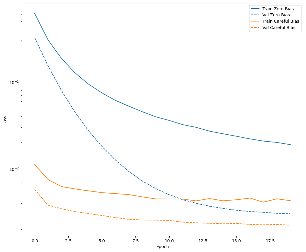
The above figure makes it clear: In terms of validation loss, on this problem, this careful initialization gives a clear advantage.
Train the model
model = make_model()
model.load_weights(initial_weights)
baseline_history = model.fit(
    train_features,
    train_labels,
    batch_size=BATCH_SIZE,
    epochs=EPOCHS,
    callbacks=[early_stopping()],
    validation_data=(val_features, val_labels))
Epoch 1/100
90/90 ━━━━━━━━━━━━━━━━━━━━ 7s 44ms/step - Brier score: 0.0013 - accuracy: 0.9986 - auc: 0.8236 - cross entropy: 0.0082 - fn: 158.8681 - fp: 50.0989 - loss: 0.0123 - prc: 0.4019 - precision: 0.6206 - recall: 0.3733 - tn: 139423.9375 - tp: 76.6703 - val_Brier score: 0.0011 - val_accuracy: 0.9984 - val_auc: 0.9384 - val_cross entropy: 0.0054 - val_fn: 70.0000 - val_fp: 1.0000 - val_loss: 0.0054 - val_prc: 0.7641 - val_precision: 0.9231 - val_recall: 0.1463 - val_tn: 45486.0000 - val_tp: 12.0000
Epoch 2/100
90/90 ━━━━━━━━━━━━━━━━━━━━ 0s 3ms/step - Brier score: 0.0011 - accuracy: 0.9988 - auc: 0.8707 - cross entropy: 0.0073 - fn: 96.2308 - fp: 15.1319 - loss: 0.0073 - prc: 0.4775 - precision: 0.8256 - recall: 0.4258 - tn: 93963.4297 - tp: 65.7802 - val_Brier score: 6.3164e-04 - val_accuracy: 0.9993 - val_auc: 0.9327 - val_cross entropy: 0.0039 - val_fn: 28.0000 - val_fp: 6.0000 - val_loss: 0.0039 - val_prc: 0.7800 - val_precision: 0.9000 - val_recall: 0.6585 - val_tn: 45481.0000 - val_tp: 54.0000
Epoch 3/100
90/90 ━━━━━━━━━━━━━━━━━━━━ 0s 4ms/step - Brier score: 0.0010 - accuracy: 0.9988 - auc: 0.8568 - cross entropy: 0.0064 - fn: 96.9670 - fp: 22.6703 - loss: 0.0064 - prc: 0.4659 - precision: 0.6843 - recall: 0.3704 - tn: 93960.5859 - tp: 60.3517 - val_Brier score: 5.2946e-04 - val_accuracy: 0.9994 - val_auc: 0.9327 - val_cross entropy: 0.0034 - val_fn: 22.0000 - val_fp: 7.0000 - val_loss: 0.0034 - val_prc: 0.8030 - val_precision: 0.8955 - val_recall: 0.7317 - val_tn: 45480.0000 - val_tp: 60.0000
Epoch 4/100
90/90 ━━━━━━━━━━━━━━━━━━━━ 0s 3ms/step - Brier score: 8.3760e-04 - accuracy: 0.9990 - auc: 0.9158 - cross entropy: 0.0052 - fn: 78.3736 - fp: 16.5714 - loss: 0.0052 - prc: 0.5847 - precision: 0.7786 - recall: 0.4360 - tn: 93971.8984 - tp: 73.7253 - val_Brier score: 5.1657e-04 - val_accuracy: 0.9994 - val_auc: 0.9328 - val_cross entropy: 0.0032 - val_fn: 20.0000 - val_fp: 7.0000 - val_loss: 0.0032 - val_prc: 0.8076 - val_precision: 0.8986 - val_recall: 0.7561 - val_tn: 45480.0000 - val_tp: 62.0000
Epoch 5/100
90/90 ━━━━━━━━━━━━━━━━━━━━ 0s 4ms/step - Brier score: 9.0654e-04 - accuracy: 0.9989 - auc: 0.8996 - cross entropy: 0.0054 - fn: 79.9890 - fp: 17.5714 - loss: 0.0054 - prc: 0.6563 - precision: 0.8161 - recall: 0.4906 - tn: 93961.6562 - tp: 81.3516 - val_Brier score: 4.8831e-04 - val_accuracy: 0.9995 - val_auc: 0.9328 - val_cross entropy: 0.0030 - val_fn: 18.0000 - val_fp: 7.0000 - val_loss: 0.0030 - val_prc: 0.8190 - val_precision: 0.9014 - val_recall: 0.7805 - val_tn: 45480.0000 - val_tp: 64.0000
Epoch 6/100
90/90 ━━━━━━━━━━━━━━━━━━━━ 0s 3ms/step - Brier score: 9.5687e-04 - accuracy: 0.9989 - auc: 0.8888 - cross entropy: 0.0057 - fn: 80.5934 - fp: 20.6374 - loss: 0.0057 - prc: 0.5832 - precision: 0.7764 - recall: 0.4924 - tn: 93959.9766 - tp: 79.3626 - val_Brier score: 4.8348e-04 - val_accuracy: 0.9994 - val_auc: 0.9327 - val_cross entropy: 0.0029 - val_fn: 19.0000 - val_fp: 7.0000 - val_loss: 0.0029 - val_prc: 0.8328 - val_precision: 0.9000 - val_recall: 0.7683 - val_tn: 45480.0000 - val_tp: 63.0000
Epoch 7/100
90/90 ━━━━━━━━━━━━━━━━━━━━ 0s 3ms/step - Brier score: 9.6310e-04 - accuracy: 0.9989 - auc: 0.9151 - cross entropy: 0.0054 - fn: 79.7912 - fp: 19.9341 - loss: 0.0054 - prc: 0.6522 - precision: 0.7985 - recall: 0.5236 - tn: 93953.0469 - tp: 87.8022 - val_Brier score: 4.6162e-04 - val_accuracy: 0.9995 - val_auc: 0.9449 - val_cross entropy: 0.0028 - val_fn: 16.0000 - val_fp: 8.0000 - val_loss: 0.0028 - val_prc: 0.8431 - val_precision: 0.8919 - val_recall: 0.8049 - val_tn: 45479.0000 - val_tp: 66.0000
Epoch 8/100
90/90 ━━━━━━━━━━━━━━━━━━━━ 0s 3ms/step - Brier score: 8.9193e-04 - accuracy: 0.9990 - auc: 0.8859 - cross entropy: 0.0054 - fn: 72.3516 - fp: 18.9670 - loss: 0.0054 - prc: 0.6052 - precision: 0.8055 - recall: 0.5336 - tn: 93962.6172 - tp: 86.6374 - val_Brier score: 4.4717e-04 - val_accuracy: 0.9995 - val_auc: 0.9509 - val_cross entropy: 0.0027 - val_fn: 16.0000 - val_fp: 8.0000 - val_loss: 0.0027 - val_prc: 0.8545 - val_precision: 0.8919 - val_recall: 0.8049 - val_tn: 45479.0000 - val_tp: 66.0000
Epoch 9/100
90/90 ━━━━━━━━━━━━━━━━━━━━ 0s 3ms/step - Brier score: 8.3613e-04 - accuracy: 0.9990 - auc: 0.8997 - cross entropy: 0.0049 - fn: 73.0000 - fp: 19.3956 - loss: 0.0049 - prc: 0.6382 - precision: 0.8158 - recall: 0.5571 - tn: 93956.5312 - tp: 91.6484 - val_Brier score: 4.3421e-04 - val_accuracy: 0.9995 - val_auc: 0.9571 - val_cross entropy: 0.0025 - val_fn: 16.0000 - val_fp: 8.0000 - val_loss: 0.0025 - val_prc: 0.8708 - val_precision: 0.8919 - val_recall: 0.8049 - val_tn: 45479.0000 - val_tp: 66.0000
Epoch 10/100
90/90 ━━━━━━━━━━━━━━━━━━━━ 0s 3ms/step - Brier score: 8.2062e-04 - accuracy: 0.9991 - auc: 0.9295 - cross entropy: 0.0047 - fn: 73.4615 - fp: 14.4176 - loss: 0.0047 - prc: 0.6825 - precision: 0.8762 - recall: 0.5505 - tn: 93960.9688 - tp: 91.7253 - val_Brier score: 4.3984e-04 - val_accuracy: 0.9995 - val_auc: 0.9571 - val_cross entropy: 0.0025 - val_fn: 16.0000 - val_fp: 8.0000 - val_loss: 0.0025 - val_prc: 0.8678 - val_precision: 0.8919 - val_recall: 0.8049 - val_tn: 45479.0000 - val_tp: 66.0000
Epoch 11/100
90/90 ━━━━━━━━━━━━━━━━━━━━ 0s 3ms/step - Brier score: 7.9813e-04 - accuracy: 0.9991 - auc: 0.9156 - cross entropy: 0.0044 - fn: 72.3407 - fp: 18.0659 - loss: 0.0044 - prc: 0.6653 - precision: 0.8269 - recall: 0.5163 - tn: 93971.7344 - tp: 78.4286 - val_Brier score: 4.2948e-04 - val_accuracy: 0.9995 - val_auc: 0.9631 - val_cross entropy: 0.0025 - val_fn: 16.0000 - val_fp: 8.0000 - val_loss: 0.0025 - val_prc: 0.8749 - val_precision: 0.8919 - val_recall: 0.8049 - val_tn: 45479.0000 - val_tp: 66.0000
Epoch 12/100
90/90 ━━━━━━━━━━━━━━━━━━━━ 0s 3ms/step - Brier score: 7.9645e-04 - accuracy: 0.9990 - auc: 0.8946 - cross entropy: 0.0046 - fn: 67.5824 - fp: 19.9231 - loss: 0.0046 - prc: 0.6488 - precision: 0.7907 - recall: 0.5660 - tn: 93966.6719 - tp: 86.3956 - val_Brier score: 4.2749e-04 - val_accuracy: 0.9995 - val_auc: 0.9631 - val_cross entropy: 0.0025 - val_fn: 13.0000 - val_fp: 8.0000 - val_loss: 0.0025 - val_prc: 0.8747 - val_precision: 0.8961 - val_recall: 0.8415 - val_tn: 45479.0000 - val_tp: 69.0000
Epoch 13/100
90/90 ━━━━━━━━━━━━━━━━━━━━ 0s 3ms/step - Brier score: 7.9827e-04 - accuracy: 0.9990 - auc: 0.9186 - cross entropy: 0.0047 - fn: 67.0220 - fp: 22.9341 - loss: 0.0047 - prc: 0.6959 - precision: 0.8234 - recall: 0.5924 - tn: 93951.3984 - tp: 99.2198 - val_Brier score: 4.1913e-04 - val_accuracy: 0.9995 - val_auc: 0.9631 - val_cross entropy: 0.0024 - val_fn: 14.0000 - val_fp: 8.0000 - val_loss: 0.0024 - val_prc: 0.8769 - val_precision: 0.8947 - val_recall: 0.8293 - val_tn: 45479.0000 - val_tp: 68.0000
Epoch 14/100
90/90 ━━━━━━━━━━━━━━━━━━━━ 0s 4ms/step - Brier score: 6.9193e-04 - accuracy: 0.9992 - auc: 0.8996 - cross entropy: 0.0043 - fn: 60.7692 - fp: 15.8462 - loss: 0.0043 - prc: 0.7059 - precision: 0.8820 - recall: 0.6140 - tn: 93964.6172 - tp: 99.3407 - val_Brier score: 4.0537e-04 - val_accuracy: 0.9995 - val_auc: 0.9571 - val_cross entropy: 0.0024 - val_fn: 14.0000 - val_fp: 8.0000 - val_loss: 0.0024 - val_prc: 0.8751 - val_precision: 0.8947 - val_recall: 0.8293 - val_tn: 45479.0000 - val_tp: 68.0000
Epoch 15/100
90/90 ━━━━━━━━━━━━━━━━━━━━ 0s 4ms/step - Brier score: 8.7191e-04 - accuracy: 0.9990 - auc: 0.9083 - cross entropy: 0.0048 - fn: 73.3297 - fp: 16.7253 - loss: 0.0048 - prc: 0.6461 - precision: 0.8193 - recall: 0.4967 - tn: 93966.0078 - tp: 84.5055 - val_Brier score: 4.0166e-04 - val_accuracy: 0.9995 - val_auc: 0.9631 - val_cross entropy: 0.0023 - val_fn: 14.0000 - val_fp: 8.0000 - val_loss: 0.0023 - val_prc: 0.8796 - val_precision: 0.8947 - val_recall: 0.8293 - val_tn: 45479.0000 - val_tp: 68.0000
Epoch 16/100
90/90 ━━━━━━━━━━━━━━━━━━━━ 0s 3ms/step - Brier score: 7.7092e-04 - accuracy: 0.9991 - auc: 0.9261 - cross entropy: 0.0042 - fn: 65.2308 - fp: 18.3187 - loss: 0.0042 - prc: 0.7057 - precision: 0.8384 - recall: 0.6026 - tn: 93959.4844 - tp: 97.5385 - val_Brier score: 3.9099e-04 - val_accuracy: 0.9995 - val_auc: 0.9631 - val_cross entropy: 0.0023 - val_fn: 14.0000 - val_fp: 8.0000 - val_loss: 0.0023 - val_prc: 0.8793 - val_precision: 0.8947 - val_recall: 0.8293 - val_tn: 45479.0000 - val_tp: 68.0000
Epoch 17/100
90/90 ━━━━━━━━━━━━━━━━━━━━ 0s 3ms/step - Brier score: 6.7751e-04 - accuracy: 0.9992 - auc: 0.9493 - cross entropy: 0.0036 - fn: 60.1648 - fp: 19.0440 - loss: 0.0036 - prc: 0.7219 - precision: 0.8393 - recall: 0.6479 - tn: 93965.7891 - tp: 95.5714 - val_Brier score: 3.9969e-04 - val_accuracy: 0.9995 - val_auc: 0.9631 - val_cross entropy: 0.0023 - val_fn: 13.0000 - val_fp: 8.0000 - val_loss: 0.0023 - val_prc: 0.8798 - val_precision: 0.8961 - val_recall: 0.8415 - val_tn: 45479.0000 - val_tp: 69.0000
Epoch 18/100
90/90 ━━━━━━━━━━━━━━━━━━━━ 0s 3ms/step - Brier score: 6.7281e-04 - accuracy: 0.9992 - auc: 0.9265 - cross entropy: 0.0038 - fn: 56.6483 - fp: 21.4066 - loss: 0.0038 - prc: 0.7349 - precision: 0.8293 - recall: 0.6590 - tn: 93963.6016 - tp: 98.9121 - val_Brier score: 3.8850e-04 - val_accuracy: 0.9995 - val_auc: 0.9631 - val_cross entropy: 0.0023 - val_fn: 14.0000 - val_fp: 8.0000 - val_loss: 0.0023 - val_prc: 0.8806 - val_precision: 0.8947 - val_recall: 0.8293 - val_tn: 45479.0000 - val_tp: 68.0000
Epoch 19/100
90/90 ━━━━━━━━━━━━━━━━━━━━ 0s 3ms/step - Brier score: 8.2819e-04 - accuracy: 0.9991 - auc: 0.9152 - cross entropy: 0.0045 - fn: 68.9670 - fp: 16.4615 - loss: 0.0045 - prc: 0.7070 - precision: 0.8723 - recall: 0.5674 - tn: 93961.1875 - tp: 93.9560 - val_Brier score: 3.7945e-04 - val_accuracy: 0.9996 - val_auc: 0.9632 - val_cross entropy: 0.0022 - val_fn: 15.0000 - val_fp: 4.0000 - val_loss: 0.0022 - val_prc: 0.8846 - val_precision: 0.9437 - val_recall: 0.8171 - val_tn: 45483.0000 - val_tp: 67.0000
Epoch 20/100
90/90 ━━━━━━━━━━━━━━━━━━━━ 0s 3ms/step - Brier score: 7.3339e-04 - accuracy: 0.9991 - auc: 0.9177 - cross entropy: 0.0040 - fn: 69.4066 - fp: 15.1868 - loss: 0.0040 - prc: 0.7302 - precision: 0.8563 - recall: 0.5912 - tn: 93962.6797 - tp: 93.2967 - val_Brier score: 3.9398e-04 - val_accuracy: 0.9996 - val_auc: 0.9631 - val_cross entropy: 0.0023 - val_fn: 12.0000 - val_fp: 8.0000 - val_loss: 0.0023 - val_prc: 0.8820 - val_precision: 0.8974 - val_recall: 0.8537 - val_tn: 45479.0000 - val_tp: 70.0000
Epoch 21/100
90/90 ━━━━━━━━━━━━━━━━━━━━ 0s 3ms/step - Brier score: 6.4973e-04 - accuracy: 0.9992 - auc: 0.9275 - cross entropy: 0.0037 - fn: 58.8681 - fp: 16.9231 - loss: 0.0037 - prc: 0.7428 - precision: 0.8653 - recall: 0.6408 - tn: 93966.9141 - tp: 97.8681 - val_Brier score: 3.7917e-04 - val_accuracy: 0.9996 - val_auc: 0.9631 - val_cross entropy: 0.0022 - val_fn: 13.0000 - val_fp: 6.0000 - val_loss: 0.0022 - val_prc: 0.8842 - val_precision: 0.9200 - val_recall: 0.8415 - val_tn: 45481.0000 - val_tp: 69.0000
Epoch 22/100
90/90 ━━━━━━━━━━━━━━━━━━━━ 0s 3ms/step - Brier score: 7.8078e-04 - accuracy: 0.9991 - auc: 0.9217 - cross entropy: 0.0043 - fn: 65.3407 - fp: 17.4835 - loss: 0.0043 - prc: 0.7030 - precision: 0.8490 - recall: 0.5930 - tn: 93957.4062 - tp: 100.3407 - val_Brier score: 3.6988e-04 - val_accuracy: 0.9996 - val_auc: 0.9632 - val_cross entropy: 0.0022 - val_fn: 15.0000 - val_fp: 4.0000 - val_loss: 0.0022 - val_prc: 0.8860 - val_precision: 0.9437 - val_recall: 0.8171 - val_tn: 45483.0000 - val_tp: 67.0000
Epoch 23/100
90/90 ━━━━━━━━━━━━━━━━━━━━ 0s 3ms/step - Brier score: 6.5680e-04 - accuracy: 0.9992 - auc: 0.9284 - cross entropy: 0.0037 - fn: 59.4396 - fp: 16.5934 - loss: 0.0037 - prc: 0.7232 - precision: 0.8467 - recall: 0.6442 - tn: 93967.9141 - tp: 96.6264 - val_Brier score: 3.8501e-04 - val_accuracy: 0.9996 - val_auc: 0.9632 - val_cross entropy: 0.0022 - val_fn: 12.0000 - val_fp: 8.0000 - val_loss: 0.0022 - val_prc: 0.8874 - val_precision: 0.8974 - val_recall: 0.8537 - val_tn: 45479.0000 - val_tp: 70.0000
Epoch 24/100
90/90 ━━━━━━━━━━━━━━━━━━━━ 0s 3ms/step - Brier score: 7.6319e-04 - accuracy: 0.9991 - auc: 0.9350 - cross entropy: 0.0042 - fn: 62.4835 - fp: 18.8681 - loss: 0.0042 - prc: 0.7144 - precision: 0.8168 - recall: 0.6266 - tn: 93958.2656 - tp: 100.9560 - val_Brier score: 3.7177e-04 - val_accuracy: 0.9996 - val_auc: 0.9571 - val_cross entropy: 0.0022 - val_fn: 13.0000 - val_fp: 4.0000 - val_loss: 0.0022 - val_prc: 0.8853 - val_precision: 0.9452 - val_recall: 0.8415 - val_tn: 45483.0000 - val_tp: 69.0000
Epoch 25/100
90/90 ━━━━━━━━━━━━━━━━━━━━ 0s 3ms/step - Brier score: 7.7663e-04 - accuracy: 0.9991 - auc: 0.9317 - cross entropy: 0.0041 - fn: 64.8681 - fp: 16.8901 - loss: 0.0041 - prc: 0.7062 - precision: 0.8374 - recall: 0.5877 - tn: 93961.2734 - tp: 97.5385 - val_Brier score: 3.6719e-04 - val_accuracy: 0.9996 - val_auc: 0.9571 - val_cross entropy: 0.0022 - val_fn: 16.0000 - val_fp: 4.0000 - val_loss: 0.0022 - val_prc: 0.8856 - val_precision: 0.9429 - val_recall: 0.8049 - val_tn: 45483.0000 - val_tp: 66.0000
Epoch 26/100
90/90 ━━━━━━━━━━━━━━━━━━━━ 0s 3ms/step - Brier score: 7.6326e-04 - accuracy: 0.9991 - auc: 0.9250 - cross entropy: 0.0041 - fn: 68.6813 - fp: 16.3297 - loss: 0.0041 - prc: 0.7517 - precision: 0.8644 - recall: 0.6002 - tn: 93955.5312 - tp: 100.0330 - val_Brier score: 3.8389e-04 - val_accuracy: 0.9996 - val_auc: 0.9571 - val_cross entropy: 0.0022 - val_fn: 12.0000 - val_fp: 8.0000 - val_loss: 0.0022 - val_prc: 0.8845 - val_precision: 0.8974 - val_recall: 0.8537 - val_tn: 45479.0000 - val_tp: 70.0000
Epoch 27/100
90/90 ━━━━━━━━━━━━━━━━━━━━ 0s 3ms/step - Brier score: 7.8576e-04 - accuracy: 0.9991 - auc: 0.9288 - cross entropy: 0.0042 - fn: 61.5165 - fp: 18.7802 - loss: 0.0042 - prc: 0.6859 - precision: 0.8108 - recall: 0.5962 - tn: 93959.4844 - tp: 100.7912 - val_Brier score: 3.6900e-04 - val_accuracy: 0.9996 - val_auc: 0.9632 - val_cross entropy: 0.0021 - val_fn: 12.0000 - val_fp: 6.0000 - val_loss: 0.0021 - val_prc: 0.8899 - val_precision: 0.9211 - val_recall: 0.8537 - val_tn: 45481.0000 - val_tp: 70.0000
Epoch 28/100
90/90 ━━━━━━━━━━━━━━━━━━━━ 0s 3ms/step - Brier score: 8.3276e-04 - accuracy: 0.9991 - auc: 0.9218 - cross entropy: 0.0044 - fn: 65.2527 - fp: 19.2308 - loss: 0.0044 - prc: 0.6487 - precision: 0.7912 - recall: 0.5671 - tn: 93963.1953 - tp: 92.8901 - val_Brier score: 3.6730e-04 - val_accuracy: 0.9996 - val_auc: 0.9571 - val_cross entropy: 0.0022 - val_fn: 12.0000 - val_fp: 5.0000 - val_loss: 0.0022 - val_prc: 0.8855 - val_precision: 0.9333 - val_recall: 0.8537 - val_tn: 45482.0000 - val_tp: 70.0000
Epoch 29/100
90/90 ━━━━━━━━━━━━━━━━━━━━ 0s 3ms/step - Brier score: 6.6513e-04 - accuracy: 0.9992 - auc: 0.9247 - cross entropy: 0.0036 - fn: 61.8352 - fp: 14.6923 - loss: 0.0036 - prc: 0.7626 - precision: 0.8972 - recall: 0.6181 - tn: 93964.9375 - tp: 99.1099 - val_Brier score: 3.6506e-04 - val_accuracy: 0.9996 - val_auc: 0.9571 - val_cross entropy: 0.0021 - val_fn: 12.0000 - val_fp: 5.0000 - val_loss: 0.0021 - val_prc: 0.8872 - val_precision: 0.9333 - val_recall: 0.8537 - val_tn: 45482.0000 - val_tp: 70.0000
Epoch 30/100
90/90 ━━━━━━━━━━━━━━━━━━━━ 0s 3ms/step - Brier score: 7.1007e-04 - accuracy: 0.9991 - auc: 0.9455 - cross entropy: 0.0036 - fn: 60.5385 - fp: 16.3956 - loss: 0.0036 - prc: 0.7654 - precision: 0.8556 - recall: 0.6277 - tn: 93963.3984 - tp: 100.2418 - val_Brier score: 3.6817e-04 - val_accuracy: 0.9996 - val_auc: 0.9571 - val_cross entropy: 0.0021 - val_fn: 12.0000 - val_fp: 6.0000 - val_loss: 0.0021 - val_prc: 0.8868 - val_precision: 0.9211 - val_recall: 0.8537 - val_tn: 45481.0000 - val_tp: 70.0000
Epoch 31/100
90/90 ━━━━━━━━━━━━━━━━━━━━ 0s 3ms/step - Brier score: 7.0085e-04 - accuracy: 0.9991 - auc: 0.9130 - cross entropy: 0.0039 - fn: 63.7363 - fp: 20.1429 - loss: 0.0039 - prc: 0.7108 - precision: 0.8159 - recall: 0.5851 - tn: 93967.3516 - tp: 89.3407 - val_Brier score: 3.6721e-04 - val_accuracy: 0.9996 - val_auc: 0.9571 - val_cross entropy: 0.0021 - val_fn: 12.0000 - val_fp: 6.0000 - val_loss: 0.0021 - val_prc: 0.8871 - val_precision: 0.9211 - val_recall: 0.8537 - val_tn: 45481.0000 - val_tp: 70.0000
Epoch 32/100
90/90 ━━━━━━━━━━━━━━━━━━━━ 0s 3ms/step - Brier score: 7.2889e-04 - accuracy: 0.9992 - auc: 0.9260 - cross entropy: 0.0042 - fn: 64.7473 - fp: 17.0000 - loss: 0.0042 - prc: 0.6922 - precision: 0.8590 - recall: 0.6338 - tn: 93959.4297 - tp: 99.3956 - val_Brier score: 3.6700e-04 - val_accuracy: 0.9996 - val_auc: 0.9571 - val_cross entropy: 0.0022 - val_fn: 12.0000 - val_fp: 6.0000 - val_loss: 0.0022 - val_prc: 0.8861 - val_precision: 0.9211 - val_recall: 0.8537 - val_tn: 45481.0000 - val_tp: 70.0000
Epoch 33/100
90/90 ━━━━━━━━━━━━━━━━━━━━ 0s 3ms/step - Brier score: 7.6838e-04 - accuracy: 0.9991 - auc: 0.9147 - cross entropy: 0.0043 - fn: 62.1758 - fp: 19.4615 - loss: 0.0043 - prc: 0.7076 - precision: 0.8379 - recall: 0.6039 - tn: 93964.6172 - tp: 94.3187 - val_Brier score: 3.5868e-04 - val_accuracy: 0.9996 - val_auc: 0.9571 - val_cross entropy: 0.0021 - val_fn: 15.0000 - val_fp: 4.0000 - val_loss: 0.0021 - val_prc: 0.8888 - val_precision: 0.9437 - val_recall: 0.8171 - val_tn: 45483.0000 - val_tp: 67.0000
Epoch 34/100
90/90 ━━━━━━━━━━━━━━━━━━━━ 0s 3ms/step - Brier score: 7.1733e-04 - accuracy: 0.9992 - auc: 0.9340 - cross entropy: 0.0038 - fn: 56.5934 - fp: 16.9560 - loss: 0.0038 - prc: 0.7449 - precision: 0.8692 - recall: 0.6213 - tn: 93963.1562 - tp: 103.8681 - val_Brier score: 3.5923e-04 - val_accuracy: 0.9996 - val_auc: 0.9571 - val_cross entropy: 0.0021 - val_fn: 15.0000 - val_fp: 4.0000 - val_loss: 0.0021 - val_prc: 0.8886 - val_precision: 0.9437 - val_recall: 0.8171 - val_tn: 45483.0000 - val_tp: 67.0000
Epoch 35/100
90/90 ━━━━━━━━━━━━━━━━━━━━ 0s 4ms/step - Brier score: 7.7370e-04 - accuracy: 0.9991 - auc: 0.9391 - cross entropy: 0.0040 - fn: 65.4835 - fp: 16.2308 - loss: 0.0040 - prc: 0.7310 - precision: 0.8463 - recall: 0.5861 - tn: 93961.7578 - tp: 97.0989 - val_Brier score: 3.6408e-04 - val_accuracy: 0.9996 - val_auc: 0.9632 - val_cross entropy: 0.0021 - val_fn: 12.0000 - val_fp: 5.0000 - val_loss: 0.0021 - val_prc: 0.8937 - val_precision: 0.9333 - val_recall: 0.8537 - val_tn: 45482.0000 - val_tp: 70.0000
Epoch 36/100
90/90 ━━━━━━━━━━━━━━━━━━━━ 0s 3ms/step - Brier score: 6.7652e-04 - accuracy: 0.9992 - auc: 0.9293 - cross entropy: 0.0038 - fn: 59.1758 - fp: 15.4066 - loss: 0.0038 - prc: 0.7030 - precision: 0.8639 - recall: 0.6167 - tn: 93971.2969 - tp: 94.6923 - val_Brier score: 3.7391e-04 - val_accuracy: 0.9996 - val_auc: 0.9632 - val_cross entropy: 0.0022 - val_fn: 12.0000 - val_fp: 6.0000 - val_loss: 0.0022 - val_prc: 0.8934 - val_precision: 0.9211 - val_recall: 0.8537 - val_tn: 45481.0000 - val_tp: 70.0000
Epoch 37/100
90/90 ━━━━━━━━━━━━━━━━━━━━ 0s 3ms/step - Brier score: 7.3074e-04 - accuracy: 0.9992 - auc: 0.9428 - cross entropy: 0.0037 - fn: 60.7802 - fp: 17.3626 - loss: 0.0037 - prc: 0.7377 - precision: 0.8461 - recall: 0.6337 - tn: 93962.8438 - tp: 99.5824 - val_Brier score: 3.6460e-04 - val_accuracy: 0.9996 - val_auc: 0.9571 - val_cross entropy: 0.0021 - val_fn: 12.0000 - val_fp: 5.0000 - val_loss: 0.0021 - val_prc: 0.8902 - val_precision: 0.9333 - val_recall: 0.8537 - val_tn: 45482.0000 - val_tp: 70.0000
Epoch 38/100
90/90 ━━━━━━━━━━━━━━━━━━━━ 0s 3ms/step - Brier score: 6.6683e-04 - accuracy: 0.9993 - auc: 0.9190 - cross entropy: 0.0037 - fn: 52.7912 - fp: 14.1868 - loss: 0.0037 - prc: 0.7344 - precision: 0.8774 - recall: 0.6506 - tn: 93971.1953 - tp: 102.3956 - val_Brier score: 3.6012e-04 - val_accuracy: 0.9996 - val_auc: 0.9571 - val_cross entropy: 0.0021 - val_fn: 12.0000 - val_fp: 5.0000 - val_loss: 0.0021 - val_prc: 0.8892 - val_precision: 0.9333 - val_recall: 0.8537 - val_tn: 45482.0000 - val_tp: 70.0000
Epoch 39/100
90/90 ━━━━━━━━━━━━━━━━━━━━ 0s 3ms/step - Brier score: 6.7595e-04 - accuracy: 0.9992 - auc: 0.9244 - cross entropy: 0.0036 - fn: 59.9890 - fp: 15.4176 - loss: 0.0036 - prc: 0.7161 - precision: 0.8446 - recall: 0.5989 - tn: 93972.8906 - tp: 92.2747 - val_Brier score: 3.6358e-04 - val_accuracy: 0.9996 - val_auc: 0.9571 - val_cross entropy: 0.0021 - val_fn: 12.0000 - val_fp: 5.0000 - val_loss: 0.0021 - val_prc: 0.8890 - val_precision: 0.9333 - val_recall: 0.8537 - val_tn: 45482.0000 - val_tp: 70.0000
Epoch 40/100
90/90 ━━━━━━━━━━━━━━━━━━━━ 0s 4ms/step - Brier score: 6.4591e-04 - accuracy: 0.9992 - auc: 0.9358 - cross entropy: 0.0036 - fn: 59.4506 - fp: 16.2747 - loss: 0.0036 - prc: 0.7248 - precision: 0.8518 - recall: 0.6376 - tn: 93967.5078 - tp: 97.3407 - val_Brier score: 3.5726e-04 - val_accuracy: 0.9996 - val_auc: 0.9632 - val_cross entropy: 0.0021 - val_fn: 14.0000 - val_fp: 4.0000 - val_loss: 0.0021 - val_prc: 0.8938 - val_precision: 0.9444 - val_recall: 0.8293 - val_tn: 45483.0000 - val_tp: 68.0000
Epoch 41/100
90/90 ━━━━━━━━━━━━━━━━━━━━ 0s 4ms/step - Brier score: 6.5670e-04 - accuracy: 0.9993 - auc: 0.9301 - cross entropy: 0.0036 - fn: 54.7582 - fp: 16.5494 - loss: 0.0036 - prc: 0.7288 - precision: 0.8547 - recall: 0.6463 - tn: 93973.3281 - tp: 95.9341 - val_Brier score: 3.5593e-04 - val_accuracy: 0.9996 - val_auc: 0.9632 - val_cross entropy: 0.0021 - val_fn: 12.0000 - val_fp: 4.0000 - val_loss: 0.0021 - val_prc: 0.8933 - val_precision: 0.9459 - val_recall: 0.8537 - val_tn: 45483.0000 - val_tp: 70.0000
Epoch 42/100
90/90 ━━━━━━━━━━━━━━━━━━━━ 0s 4ms/step - Brier score: 7.4028e-04 - accuracy: 0.9992 - auc: 0.9187 - cross entropy: 0.0040 - fn: 61.0769 - fp: 15.6593 - loss: 0.0040 - prc: 0.7178 - precision: 0.8634 - recall: 0.6371 - tn: 93964.6172 - tp: 99.2198 - val_Brier score: 3.5573e-04 - val_accuracy: 0.9996 - val_auc: 0.9632 - val_cross entropy: 0.0021 - val_fn: 15.0000 - val_fp: 3.0000 - val_loss: 0.0021 - val_prc: 0.8955 - val_precision: 0.9571 - val_recall: 0.8171 - val_tn: 45484.0000 - val_tp: 67.0000
Epoch 43/100
90/90 ━━━━━━━━━━━━━━━━━━━━ 0s 4ms/step - Brier score: 7.4173e-04 - accuracy: 0.9991 - auc: 0.9276 - cross entropy: 0.0039 - fn: 67.1099 - fp: 13.5165 - loss: 0.0039 - prc: 0.7369 - precision: 0.8910 - recall: 0.5853 - tn: 93963.0469 - tp: 96.9011 - val_Brier score: 3.5516e-04 - val_accuracy: 0.9996 - val_auc: 0.9632 - val_cross entropy: 0.0021 - val_fn: 15.0000 - val_fp: 3.0000 - val_loss: 0.0021 - val_prc: 0.8967 - val_precision: 0.9571 - val_recall: 0.8171 - val_tn: 45484.0000 - val_tp: 67.0000
Epoch 44/100
90/90 ━━━━━━━━━━━━━━━━━━━━ 0s 4ms/step - Brier score: 6.8514e-04 - accuracy: 0.9992 - auc: 0.9083 - cross entropy: 0.0041 - fn: 61.3626 - fp: 14.4176 - loss: 0.0041 - prc: 0.6952 - precision: 0.8665 - recall: 0.6305 - tn: 93966.5938 - tp: 98.1978 - val_Brier score: 3.5625e-04 - val_accuracy: 0.9996 - val_auc: 0.9632 - val_cross entropy: 0.0021 - val_fn: 14.0000 - val_fp: 4.0000 - val_loss: 0.0021 - val_prc: 0.8940 - val_precision: 0.9444 - val_recall: 0.8293 - val_tn: 45483.0000 - val_tp: 68.0000
Epoch 45/100
90/90 ━━━━━━━━━━━━━━━━━━━━ 0s 3ms/step - Brier score: 6.5736e-04 - accuracy: 0.9993 - auc: 0.9347 - cross entropy: 0.0035 - fn: 53.7363 - fp: 17.3407 - loss: 0.0035 - prc: 0.7572 - precision: 0.8641 - recall: 0.6611 - tn: 93965.4609 - tp: 104.0330 - val_Brier score: 3.5624e-04 - val_accuracy: 0.9996 - val_auc: 0.9693 - val_cross entropy: 0.0021 - val_fn: 12.0000 - val_fp: 4.0000 - val_loss: 0.0021 - val_prc: 0.8999 - val_precision: 0.9459 - val_recall: 0.8537 - val_tn: 45483.0000 - val_tp: 70.0000
Epoch 46/100
90/90 ━━━━━━━━━━━━━━━━━━━━ 0s 4ms/step - Brier score: 6.4475e-04 - accuracy: 0.9992 - auc: 0.9327 - cross entropy: 0.0034 - fn: 59.7473 - fp: 16.5824 - loss: 0.0034 - prc: 0.7666 - precision: 0.8494 - recall: 0.6148 - tn: 93969.7031 - tp: 94.5385 - val_Brier score: 3.5600e-04 - val_accuracy: 0.9996 - val_auc: 0.9632 - val_cross entropy: 0.0021 - val_fn: 14.0000 - val_fp: 5.0000 - val_loss: 0.0021 - val_prc: 0.8953 - val_precision: 0.9315 - val_recall: 0.8293 - val_tn: 45482.0000 - val_tp: 68.0000
Epoch 47/100
90/90 ━━━━━━━━━━━━━━━━━━━━ 0s 4ms/step - Brier score: 6.4711e-04 - accuracy: 0.9992 - auc: 0.9535 - cross entropy: 0.0034 - fn: 56.6044 - fp: 15.2637 - loss: 0.0034 - prc: 0.7703 - precision: 0.8783 - recall: 0.6687 - tn: 93959.1797 - tp: 109.5275 - val_Brier score: 3.5447e-04 - val_accuracy: 0.9996 - val_auc: 0.9632 - val_cross entropy: 0.0021 - val_fn: 14.0000 - val_fp: 5.0000 - val_loss: 0.0021 - val_prc: 0.8957 - val_precision: 0.9315 - val_recall: 0.8293 - val_tn: 45482.0000 - val_tp: 68.0000
Epoch 48/100
90/90 ━━━━━━━━━━━━━━━━━━━━ 0s 4ms/step - Brier score: 7.0048e-04 - accuracy: 0.9992 - auc: 0.9278 - cross entropy: 0.0035 - fn: 62.0110 - fp: 13.0659 - loss: 0.0035 - prc: 0.7176 - precision: 0.8421 - recall: 0.5699 - tn: 93974.2891 - tp: 91.2088 - val_Brier score: 3.5628e-04 - val_accuracy: 0.9996 - val_auc: 0.9571 - val_cross entropy: 0.0021 - val_fn: 12.0000 - val_fp: 5.0000 - val_loss: 0.0021 - val_prc: 0.8904 - val_precision: 0.9333 - val_recall: 0.8537 - val_tn: 45482.0000 - val_tp: 70.0000
Epoch 49/100
90/90 ━━━━━━━━━━━━━━━━━━━━ 0s 4ms/step - Brier score: 6.9120e-04 - accuracy: 0.9992 - auc: 0.9443 - cross entropy: 0.0036 - fn: 63.6813 - fp: 18.6593 - loss: 0.0036 - prc: 0.7408 - precision: 0.8440 - recall: 0.5999 - tn: 93963.7656 - tp: 94.4615 - val_Brier score: 3.5756e-04 - val_accuracy: 0.9996 - val_auc: 0.9571 - val_cross entropy: 0.0021 - val_fn: 12.0000 - val_fp: 5.0000 - val_loss: 0.0021 - val_prc: 0.8908 - val_precision: 0.9333 - val_recall: 0.8537 - val_tn: 45482.0000 - val_tp: 70.0000
Epoch 50/100
90/90 ━━━━━━━━━━━━━━━━━━━━ 0s 4ms/step - Brier score: 7.3006e-04 - accuracy: 0.9992 - auc: 0.9119 - cross entropy: 0.0041 - fn: 58.7473 - fp: 15.9670 - loss: 0.0041 - prc: 0.7054 - precision: 0.8526 - recall: 0.6254 - tn: 93961.4062 - tp: 104.4505 - val_Brier score: 3.5366e-04 - val_accuracy: 0.9996 - val_auc: 0.9571 - val_cross entropy: 0.0021 - val_fn: 15.0000 - val_fp: 4.0000 - val_loss: 0.0021 - val_prc: 0.8914 - val_precision: 0.9437 - val_recall: 0.8171 - val_tn: 45483.0000 - val_tp: 67.0000
Epoch 51/100
90/90 ━━━━━━━━━━━━━━━━━━━━ 0s 4ms/step - Brier score: 6.7601e-04 - accuracy: 0.9992 - auc: 0.9166 - cross entropy: 0.0040 - fn: 56.8681 - fp: 12.8901 - loss: 0.0040 - prc: 0.7306 - precision: 0.9066 - recall: 0.5950 - tn: 93974.1016 - tp: 96.7143 - val_Brier score: 3.5455e-04 - val_accuracy: 0.9996 - val_auc: 0.9632 - val_cross entropy: 0.0021 - val_fn: 12.0000 - val_fp: 5.0000 - val_loss: 0.0021 - val_prc: 0.8962 - val_precision: 0.9333 - val_recall: 0.8537 - val_tn: 45482.0000 - val_tp: 70.0000
Epoch 52/100
90/90 ━━━━━━━━━━━━━━━━━━━━ 0s 3ms/step - Brier score: 6.8761e-04 - accuracy: 0.9992 - auc: 0.9491 - cross entropy: 0.0036 - fn: 57.3626 - fp: 16.6703 - loss: 0.0036 - prc: 0.7558 - precision: 0.8728 - recall: 0.6633 - tn: 93960.0781 - tp: 106.4615 - val_Brier score: 3.5794e-04 - val_accuracy: 0.9996 - val_auc: 0.9510 - val_cross entropy: 0.0021 - val_fn: 12.0000 - val_fp: 5.0000 - val_loss: 0.0021 - val_prc: 0.8856 - val_precision: 0.9333 - val_recall: 0.8537 - val_tn: 45482.0000 - val_tp: 70.0000
Epoch 53/100
90/90 ━━━━━━━━━━━━━━━━━━━━ 0s 4ms/step - Brier score: 6.7372e-04 - accuracy: 0.9992 - auc: 0.9337 - cross entropy: 0.0039 - fn: 57.6483 - fp: 16.1758 - loss: 0.0039 - prc: 0.7352 - precision: 0.8740 - recall: 0.6468 - tn: 93962.3203 - tp: 104.4286 - val_Brier score: 3.5337e-04 - val_accuracy: 0.9996 - val_auc: 0.9510 - val_cross entropy: 0.0021 - val_fn: 15.0000 - val_fp: 4.0000 - val_loss: 0.0021 - val_prc: 0.8867 - val_precision: 0.9437 - val_recall: 0.8171 - val_tn: 45483.0000 - val_tp: 67.0000
Epoch 54/100
90/90 ━━━━━━━━━━━━━━━━━━━━ 0s 4ms/step - Brier score: 6.7745e-04 - accuracy: 0.9992 - auc: 0.9296 - cross entropy: 0.0036 - fn: 57.5275 - fp: 14.4725 - loss: 0.0036 - prc: 0.7534 - precision: 0.8939 - recall: 0.6348 - tn: 93965.9453 - tp: 102.6264 - val_Brier score: 3.5481e-04 - val_accuracy: 0.9996 - val_auc: 0.9571 - val_cross entropy: 0.0021 - val_fn: 14.0000 - val_fp: 4.0000 - val_loss: 0.0021 - val_prc: 0.8912 - val_precision: 0.9444 - val_recall: 0.8293 - val_tn: 45483.0000 - val_tp: 68.0000
Epoch 55/100
90/90 ━━━━━━━━━━━━━━━━━━━━ 0s 3ms/step - Brier score: 7.0387e-04 - accuracy: 0.9992 - auc: 0.9224 - cross entropy: 0.0038 - fn: 64.3626 - fp: 13.1429 - loss: 0.0038 - prc: 0.7406 - precision: 0.8846 - recall: 0.6024 - tn: 93966.8203 - tp: 96.2418 - val_Brier score: 3.6211e-04 - val_accuracy: 0.9996 - val_auc: 0.9632 - val_cross entropy: 0.0021 - val_fn: 12.0000 - val_fp: 5.0000 - val_loss: 0.0021 - val_prc: 0.8954 - val_precision: 0.9333 - val_recall: 0.8537 - val_tn: 45482.0000 - val_tp: 70.0000
Epoch 55: early stopping
Restoring model weights from the end of the best epoch: 45.
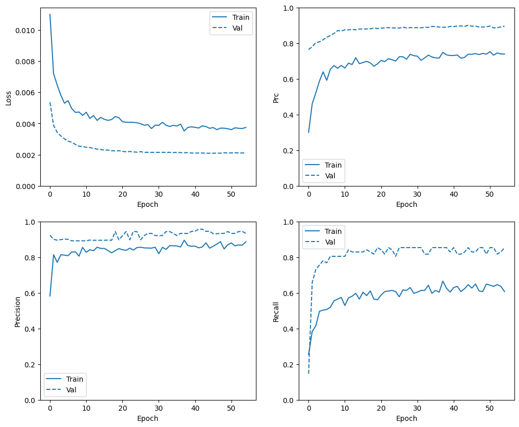
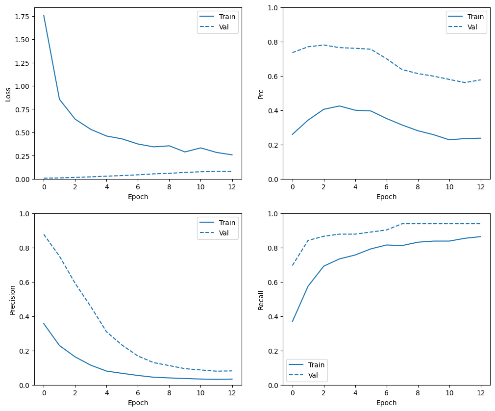
Check training history
In this section, you will produce plots of your model's accuracy and loss on the training and validation set. These are useful to check for overfitting, which you can learn more about in the Overfit and underfit tutorial.
Additionally, you can produce these plots for any of the metrics you created above. False negatives are included as an example.
def plot_metrics(history):
  metrics = ['loss', 'prc', 'precision', 'recall']
  for n, metric in enumerate(metrics):
    name = metric.replace("_"," ").capitalize()
    plt.subplot(2,2,n+1)
    plt.plot(history.epoch, history.history[metric], color=colors[0], label='Train')
    plt.plot(history.epoch, history.history['val_'+metric],
             color=colors[0], linestyle="--", label='Val')
    plt.xlabel('Epoch')
    plt.ylabel(name)
    if metric == 'loss':
      plt.ylim([0, plt.ylim()[1]])
    elif metric == 'auc':
      plt.ylim([0.8,1])
    else:
      plt.ylim([0,1])

    plt.legend()
plot_metrics(baseline_history)
Evaluate metrics
You can use a confusion matrix to summarize the actual vs. predicted labels, where the X axis is the predicted label and the Y axis is the actual label:
train_predictions_baseline = model.predict(train_features, batch_size=BATCH_SIZE)
test_predictions_baseline = model.predict(test_features, batch_size=BATCH_SIZE)
90/90 ━━━━━━━━━━━━━━━━━━━━ 0s 2ms/step
28/28 ━━━━━━━━━━━━━━━━━━━━ 0s 6ms/step
def plot_cm(labels, predictions, threshold=0.5):
  cm = confusion_matrix(labels, predictions > threshold)
  plt.figure(figsize=(5,5))
  sns.heatmap(cm, annot=True, fmt="d")
  plt.title('Confusion matrix @{:.2f}'.format(threshold))
  plt.ylabel('Actual label')
  plt.xlabel('Predicted label')

  print('Legitimate Transactions Detected (True Negatives): ', cm[0][0])
  print('Legitimate Transactions Incorrectly Detected (False Positives): ', cm[0][1])
  print('Fraudulent Transactions Missed (False Negatives): ', cm[1][0])
  print('Fraudulent Transactions Detected (True Positives): ', cm[1][1])
  print('Total Fraudulent Transactions: ', np.sum(cm[1]))
Evaluate your model on the test dataset and display the results for the metrics you created above:
baseline_results = model.evaluate(test_features, test_labels,
                                  batch_size=BATCH_SIZE, verbose=0)
for name, value in zip(model.metrics_names, baseline_results):
  print(name, ': ', value)
print()

plot_cm(test_labels, test_predictions_baseline)
loss :  0.002663512947037816
compile_metrics :  0.002663512947037816

Legitimate Transactions Detected (True Negatives):  56854
Legitimate Transactions Incorrectly Detected (False Positives):  6
Fraudulent Transactions Missed (False Negatives):  21
Fraudulent Transactions Detected (True Positives):  81
Total Fraudulent Transactions:  102

If the model had predicted everything perfectly (impossible with true randomness), this would be a diagonal matrix where values off the main diagonal, indicating incorrect predictions, would be zero. In this case, the matrix shows that you have relatively few false positives, meaning that there were relatively few legitimate transactions that were incorrectly flagged.
Changing the threshold
The default threshold of \(t=50\%\) corresponds to equal costs of false negatives and false positives. In the case of fraud detection, however, you would likely associate higher costs to false negatives than to false positives. This trade off may be preferable because false negatives would allow fraudulent transactions to go through, whereas false positives may cause an email to be sent to a customer to ask them to verify their card activity.
By decreasing the threshold, we attribute higher cost to false negatives, thereby increasing missed transactions at the price of more false positives. We test thresholds at 10% and at 1%.
plot_cm(test_labels, test_predictions_baseline, threshold=0.1)
plot_cm(test_labels, test_predictions_baseline, threshold=0.01)
Legitimate Transactions Detected (True Negatives):  56848
Legitimate Transactions Incorrectly Detected (False Positives):  12
Fraudulent Transactions Missed (False Negatives):  17
Fraudulent Transactions Detected (True Positives):  85
Total Fraudulent Transactions:  102
Legitimate Transactions Detected (True Negatives):  56789
Legitimate Transactions Incorrectly Detected (False Positives):  71
Fraudulent Transactions Missed (False Negatives):  13
Fraudulent Transactions Detected (True Positives):  89
Total Fraudulent Transactions:  102


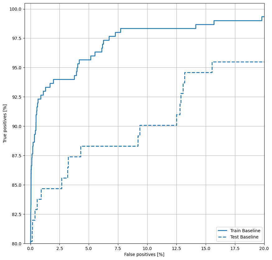
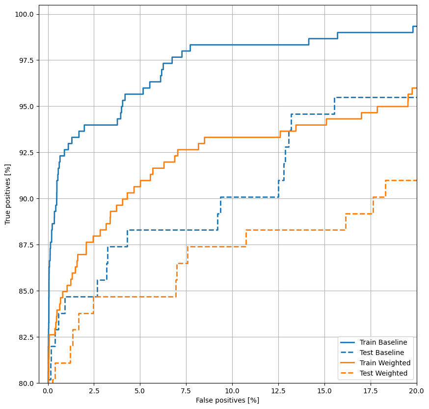
Plot the ROC
Now plot the ROC. This plot is useful because it shows, at a glance, the range of performance the model can reach by tuning the output threshold over its full range (0 to 1). So each point corresponds to a single value of the threshold.
def plot_roc(name, labels, predictions, **kwargs):
  fp, tp, _ = sklearn.metrics.roc_curve(labels, predictions)

  plt.plot(100*fp, 100*tp, label=name, linewidth=2, **kwargs)
  plt.xlabel('False positives [%]')
  plt.ylabel('True positives [%]')
  plt.xlim([-0.5,20])
  plt.ylim([80,100.5])
  plt.grid(True)
  ax = plt.gca()
  ax.set_aspect('equal')
plot_roc("Train Baseline", train_labels, train_predictions_baseline, color=colors[0])
plot_roc("Test Baseline", test_labels, test_predictions_baseline, color=colors[0], linestyle='--')
plt.legend(loc='lower right');
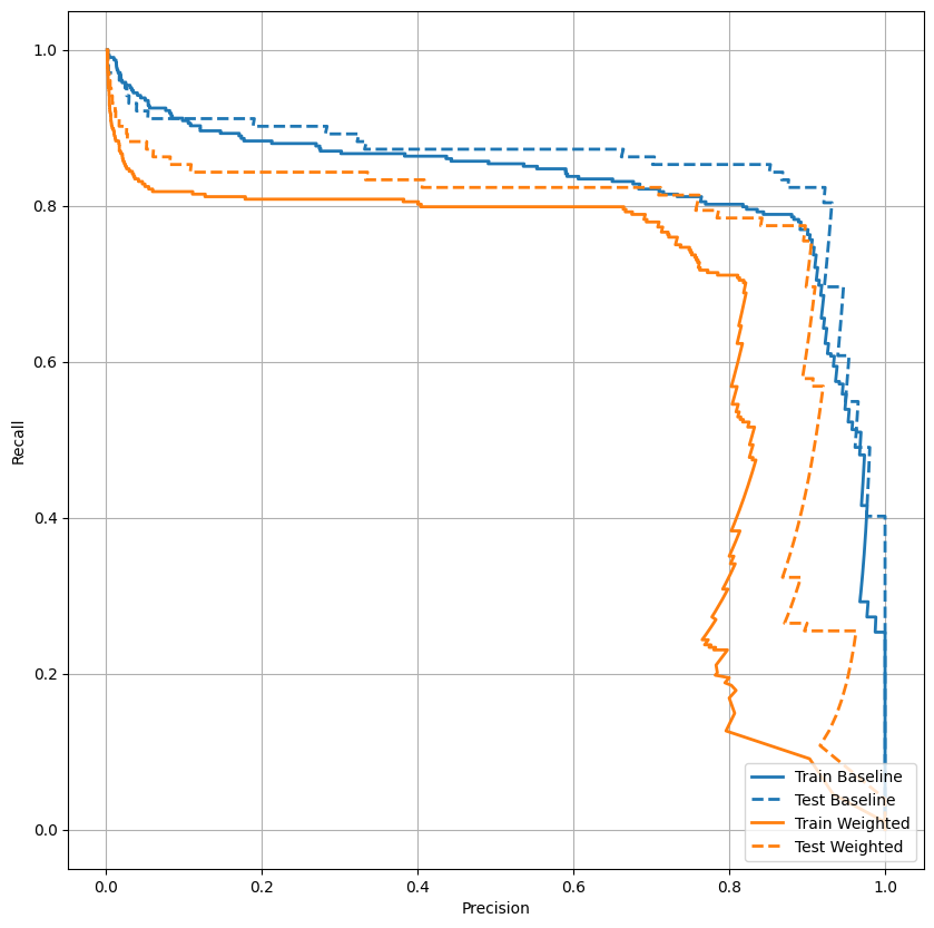
Plot the PRC
Now plot the AUPRC. Area under the interpolated precision-recall curve, obtained by plotting (recall, precision) points for different values of the classification threshold. Depending on how it's calculated, PR AUC may be equivalent to the average precision of the model.
def plot_prc(name, labels, predictions, **kwargs):
    precision, recall, _ = sklearn.metrics.precision_recall_curve(labels, predictions)

    plt.plot(precision, recall, label=name, linewidth=2, **kwargs)
    plt.xlabel('Precision')
    plt.ylabel('Recall')
    plt.grid(True)
    ax = plt.gca()
    ax.set_aspect('equal')
plot_prc("Train Baseline", train_labels, train_predictions_baseline, color=colors[0])
plot_prc("Test Baseline", test_labels, test_predictions_baseline, color=colors[0], linestyle='--')
plt.legend(loc='lower right');
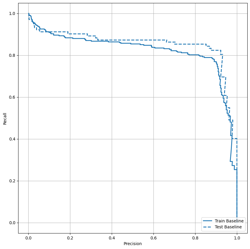
It looks like the precision is relatively high, but the recall and the area under the ROC curve (AUC) aren't as high as you might like. Classifiers often face challenges when trying to maximize both precision and recall, which is especially true when working with imbalanced datasets. It is important to consider the costs of different types of errors in the context of the problem you care about. In this example, a false negative (a fraudulent transaction is missed) may have a financial cost, while a false positive (a transaction is incorrectly flagged as fraudulent) may decrease user happiness.
Class weights
Calculate class weights
The goal is to identify fraudulent transactions, but you don't have very many of those positive samples to work with, so you would want to have the classifier heavily weight the few examples that are available. You can do this by passing Keras weights for each class through a parameter. These will cause the model to "pay more attention" to examples from an under-represented class. Note, however, that this does not increase in any way the amount of information of your dataset. In the end, using class weights is more or less equivalent to changing the output bias or to changing the threshold. Let's see how it works out.
# Scaling by total/2 helps keep the loss to a similar magnitude.
# The sum of the weights of all examples stays the same.
weight_for_0 = (1 / neg) * (total / 2.0)
weight_for_1 = (1 / pos) * (total / 2.0)

class_weight = {0: weight_for_0, 1: weight_for_1}

print('Weight for class 0: {:.2f}'.format(weight_for_0))
print('Weight for class 1: {:.2f}'.format(weight_for_1))
Weight for class 0: 0.50
Weight for class 1: 289.44
Train a model with class weights
Now try re-training and evaluating the model with class weights to see how that affects the predictions.
weighted_model = make_model()
weighted_model.load_weights(initial_weights)

weighted_history = weighted_model.fit(
    train_features,
    train_labels,
    batch_size=BATCH_SIZE,
    epochs=EPOCHS,
    callbacks=[early_stopping()],
    validation_data=(val_features, val_labels),
    # The class weights go here
    class_weight=class_weight)
Epoch 1/100
/tmpfs/src/tf_docs_env/lib/python3.9/site-packages/keras/src/layers/core/dense.py:87: UserWarning: Do not pass an `input_shape`/`input_dim` argument to a layer. When using Sequential models, prefer using an `Input(shape)` object as the first layer in the model instead.
  super().__init__(activity_regularizer=activity_regularizer, **kwargs)
90/90 ━━━━━━━━━━━━━━━━━━━━ 8s 47ms/step - Brier score: 0.0015 - accuracy: 0.9983 - auc: 0.8391 - cross entropy: 0.0094 - fn: 156.5934 - fp: 118.4505 - loss: 2.0900 - prc: 0.3940 - precision: 0.5288 - recall: 0.4313 - tn: 150723.1719 - tp: 104.3516 - val_Brier score: 6.9626e-04 - val_accuracy: 0.9993 - val_auc: 0.9530 - val_cross entropy: 0.0072 - val_fn: 25.0000 - val_fp: 8.0000 - val_loss: 0.0072 - val_prc: 0.7354 - val_precision: 0.8769 - val_recall: 0.6951 - val_tn: 45479.0000 - val_tp: 57.0000
Epoch 2/100
90/90 ━━━━━━━━━━━━━━━━━━━━ 0s 3ms/step - Brier score: 0.0034 - accuracy: 0.9963 - auc: 0.8909 - cross entropy: 0.0196 - fn: 77.0110 - fp: 278.7912 - loss: 1.0765 - prc: 0.3266 - precision: 0.2644 - recall: 0.5273 - tn: 93691.4688 - tp: 93.2967 - val_Brier score: 9.0370e-04 - val_accuracy: 0.9992 - val_auc: 0.9600 - val_cross entropy: 0.0106 - val_fn: 13.0000 - val_fp: 23.0000 - val_loss: 0.0106 - val_prc: 0.7694 - val_precision: 0.7500 - val_recall: 0.8415 - val_tn: 45464.0000 - val_tp: 69.0000
Epoch 3/100
90/90 ━━━━━━━━━━━━━━━━━━━━ 0s 3ms/step - Brier score: 0.0052 - accuracy: 0.9943 - auc: 0.9018 - cross entropy: 0.0280 - fn: 56.4945 - fp: 508.4615 - loss: 0.7222 - prc: 0.3978 - precision: 0.1789 - recall: 0.6450 - tn: 93469.3984 - tp: 106.2198 - val_Brier score: 0.0016 - val_accuracy: 0.9987 - val_auc: 0.9681 - val_cross entropy: 0.0158 - val_fn: 11.0000 - val_fp: 49.0000 - val_loss: 0.0158 - val_prc: 0.7802 - val_precision: 0.5917 - val_recall: 0.8659 - val_tn: 45438.0000 - val_tp: 71.0000
Epoch 4/100
90/90 ━━━━━━━━━━━━━━━━━━━━ 0s 3ms/step - Brier score: 0.0082 - accuracy: 0.9907 - auc: 0.8985 - cross entropy: 0.0412 - fn: 46.3956 - fp: 854.7033 - loss: 0.6114 - prc: 0.3998 - precision: 0.1116 - recall: 0.6828 - tn: 93128.9766 - tp: 110.4945 - val_Brier score: 0.0025 - val_accuracy: 0.9979 - val_auc: 0.9732 - val_cross entropy: 0.0218 - val_fn: 10.0000 - val_fp: 86.0000 - val_loss: 0.0218 - val_prc: 0.7647 - val_precision: 0.4557 - val_recall: 0.8780 - val_tn: 45401.0000 - val_tp: 72.0000
Epoch 5/100
90/90 ━━━━━━━━━━━━━━━━━━━━ 0s 3ms/step - Brier score: 0.0118 - accuracy: 0.9862 - auc: 0.9054 - cross entropy: 0.0546 - fn: 46.5934 - fp: 1299.8242 - loss: 0.6663 - prc: 0.4400 - precision: 0.0955 - recall: 0.7156 - tn: 92670.6953 - tp: 123.4615 - val_Brier score: 0.0040 - val_accuracy: 0.9962 - val_auc: 0.9780 - val_cross entropy: 0.0291 - val_fn: 10.0000 - val_fp: 161.0000 - val_loss: 0.0291 - val_prc: 0.7608 - val_precision: 0.3090 - val_recall: 0.8780 - val_tn: 45326.0000 - val_tp: 72.0000
Epoch 6/100
90/90 ━━━━━━━━━━━━━━━━━━━━ 0s 3ms/step - Brier score: 0.0152 - accuracy: 0.9821 - auc: 0.9291 - cross entropy: 0.0687 - fn: 33.1978 - fp: 1695.3627 - loss: 0.4118 - prc: 0.4045 - precision: 0.0694 - recall: 0.7888 - tn: 92289.2891 - tp: 122.7253 - val_Brier score: 0.0054 - val_accuracy: 0.9945 - val_auc: 0.9816 - val_cross entropy: 0.0356 - val_fn: 9.0000 - val_fp: 243.0000 - val_loss: 0.0356 - val_prc: 0.7555 - val_precision: 0.2310 - val_recall: 0.8902 - val_tn: 45244.0000 - val_tp: 73.0000
Epoch 7/100
90/90 ━━━━━━━━━━━━━━━━━━━━ 0s 3ms/step - Brier score: 0.0187 - accuracy: 0.9773 - auc: 0.9501 - cross entropy: 0.0816 - fn: 28.1758 - fp: 2161.0769 - loss: 0.3649 - prc: 0.4001 - precision: 0.0667 - recall: 0.8385 - tn: 91815.3203 - tp: 136.0000 - val_Brier score: 0.0073 - val_accuracy: 0.9918 - val_auc: 0.9819 - val_cross entropy: 0.0436 - val_fn: 8.0000 - val_fp: 366.0000 - val_loss: 0.0436 - val_prc: 0.6999 - val_precision: 0.1682 - val_recall: 0.9024 - val_tn: 45121.0000 - val_tp: 74.0000
Epoch 8/100
90/90 ━━━━━━━━━━━━━━━━━━━━ 0s 3ms/step - Brier score: 0.0230 - accuracy: 0.9717 - auc: 0.9505 - cross entropy: 0.0985 - fn: 30.5714 - fp: 2692.1978 - loss: 0.3364 - prc: 0.3086 - precision: 0.0454 - recall: 0.7986 - tn: 91290.4062 - tp: 127.3956 - val_Brier score: 0.0100 - val_accuracy: 0.9885 - val_auc: 0.9839 - val_cross entropy: 0.0538 - val_fn: 5.0000 - val_fp: 517.0000 - val_loss: 0.0538 - val_prc: 0.6362 - val_precision: 0.1296 - val_recall: 0.9390 - val_tn: 44970.0000 - val_tp: 77.0000
Epoch 9/100
90/90 ━━━━━━━━━━━━━━━━━━━━ 0s 3ms/step - Brier score: 0.0271 - accuracy: 0.9663 - auc: 0.9128 - cross entropy: 0.1138 - fn: 24.7473 - fp: 3137.8132 - loss: 0.4094 - prc: 0.2688 - precision: 0.0387 - recall: 0.8191 - tn: 90844.3438 - tp: 133.6703 - val_Brier score: 0.0114 - val_accuracy: 0.9865 - val_auc: 0.9853 - val_cross entropy: 0.0596 - val_fn: 5.0000 - val_fp: 609.0000 - val_loss: 0.0596 - val_prc: 0.6135 - val_precision: 0.1122 - val_recall: 0.9390 - val_tn: 44878.0000 - val_tp: 77.0000
Epoch 10/100
90/90 ━━━━━━━━━━━━━━━━━━━━ 0s 3ms/step - Brier score: 0.0289 - accuracy: 0.9642 - auc: 0.9704 - cross entropy: 0.1220 - fn: 24.0220 - fp: 3374.6594 - loss: 0.2304 - prc: 0.2944 - precision: 0.0412 - recall: 0.8665 - tn: 90603.2422 - tp: 138.6483 - val_Brier score: 0.0141 - val_accuracy: 0.9837 - val_auc: 0.9858 - val_cross entropy: 0.0697 - val_fn: 5.0000 - val_fp: 739.0000 - val_loss: 0.0697 - val_prc: 0.5984 - val_precision: 0.0944 - val_recall: 0.9390 - val_tn: 44748.0000 - val_tp: 77.0000
Epoch 11/100
90/90 ━━━━━━━━━━━━━━━━━━━━ 0s 4ms/step - Brier score: 0.0328 - accuracy: 0.9600 - auc: 0.9554 - cross entropy: 0.1394 - fn: 23.0989 - fp: 3730.7913 - loss: 0.2830 - prc: 0.2281 - precision: 0.0347 - recall: 0.8658 - tn: 90250.4062 - tp: 136.2747 - val_Brier score: 0.0158 - val_accuracy: 0.9821 - val_auc: 0.9870 - val_cross entropy: 0.0765 - val_fn: 5.0000 - val_fp: 809.0000 - val_loss: 0.0765 - val_prc: 0.5793 - val_precision: 0.0869 - val_recall: 0.9390 - val_tn: 44678.0000 - val_tp: 77.0000
Epoch 12/100
90/90 ━━━━━━━━━━━━━━━━━━━━ 0s 3ms/step - Brier score: 0.0348 - accuracy: 0.9565 - auc: 0.9489 - cross entropy: 0.1457 - fn: 25.3846 - fp: 4104.4395 - loss: 0.3314 - prc: 0.2346 - precision: 0.0340 - recall: 0.8358 - tn: 89873.6172 - tp: 137.1319 - val_Brier score: 0.0170 - val_accuracy: 0.9804 - val_auc: 0.9875 - val_cross entropy: 0.0810 - val_fn: 5.0000 - val_fp: 888.0000 - val_loss: 0.0810 - val_prc: 0.5611 - val_precision: 0.0798 - val_recall: 0.9390 - val_tn: 44599.0000 - val_tp: 77.0000
Epoch 13/100
90/90 ━━━━━━━━━━━━━━━━━━━━ 0s 3ms/step - Brier score: 0.0341 - accuracy: 0.9579 - auc: 0.9679 - cross entropy: 0.1440 - fn: 17.4615 - fp: 3938.6704 - loss: 0.2195 - prc: 0.2564 - precision: 0.0337 - recall: 0.8983 - tn: 90044.4609 - tp: 139.9780 - val_Brier score: 0.0166 - val_accuracy: 0.9808 - val_auc: 0.9879 - val_cross entropy: 0.0798 - val_fn: 5.0000 - val_fp: 868.0000 - val_loss: 0.0798 - val_prc: 0.5770 - val_precision: 0.0815 - val_recall: 0.9390 - val_tn: 44619.0000 - val_tp: 77.0000
Epoch 13: early stopping
Restoring model weights from the end of the best epoch: 3.
Check training history
plot_metrics(weighted_history)
Evaluate metrics
train_predictions_weighted = weighted_model.predict(train_features, batch_size=BATCH_SIZE)
test_predictions_weighted = weighted_model.predict(test_features, batch_size=BATCH_SIZE)
90/90 ━━━━━━━━━━━━━━━━━━━━ 0s 2ms/step
28/28 ━━━━━━━━━━━━━━━━━━━━ 0s 3ms/step
weighted_results = weighted_model.evaluate(test_features, test_labels,
                                           batch_size=BATCH_SIZE, verbose=0)
for name, value in zip(weighted_model.metrics_names, weighted_results):
  print(name, ': ', value)
print()

plot_cm(test_labels, test_predictions_weighted)
loss :  0.014986301772296429
compile_metrics :  0.014986301772296429

Legitimate Transactions Detected (True Negatives):  56817
Legitimate Transactions Incorrectly Detected (False Positives):  43
Fraudulent Transactions Missed (False Negatives):  18
Fraudulent Transactions Detected (True Positives):  84
Total Fraudulent Transactions:  102
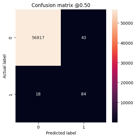
Here you can see that with class weights the accuracy and precision are lower because there are more false positives, but conversely the recall and AUC are higher because the model also found more true positives. Despite having lower accuracy, this model has higher recall (and identifies more fraudulent transactions than the baseline model at threshold 50%). Of course, there is a cost to both types of error (you wouldn't want to bug users by flagging too many legitimate transactions as fraudulent, either). Carefully consider the trade-offs between these different types of errors for your application.
Compared to the baseline model with changed threshold, the class weighted model is clearly inferior. The superiority of the baseline model is further confirmed by the lower test loss value (cross entropy and mean squared error) and additionally can be seen by plotting the ROC curves of both models together.
Plot the ROC
plot_roc("Train Baseline", train_labels, train_predictions_baseline, color=colors[0])
plot_roc("Test Baseline", test_labels, test_predictions_baseline, color=colors[0], linestyle='--')

plot_roc("Train Weighted", train_labels, train_predictions_weighted, color=colors[1])
plot_roc("Test Weighted", test_labels, test_predictions_weighted, color=colors[1], linestyle='--')


plt.legend(loc='lower right');
Plot the PRC
plot_prc("Train Baseline", train_labels, train_predictions_baseline, color=colors[0])
plot_prc("Test Baseline", test_labels, test_predictions_baseline, color=colors[0], linestyle='--')

plot_prc("Train Weighted", train_labels, train_predictions_weighted, color=colors[1])
plot_prc("Test Weighted", test_labels, test_predictions_weighted, color=colors[1], linestyle='--')


plt.legend(loc='lower right');
Oversampling
Oversample the minority class
A related approach would be to resample the dataset by oversampling the minority class.
pos_features = train_features[bool_train_labels]
neg_features = train_features[~bool_train_labels]

pos_labels = train_labels[bool_train_labels]
neg_labels = train_labels[~bool_train_labels]
Using NumPy
You can balance the dataset manually by choosing the right number of random indices from the positive examples:
ids = np.arange(len(pos_features))
choices = np.random.choice(ids, len(neg_features))

res_pos_features = pos_features[choices]
res_pos_labels = pos_labels[choices]

res_pos_features.shape
(181968, 29)
resampled_features = np.concatenate([res_pos_features, neg_features], axis=0)
resampled_labels = np.concatenate([res_pos_labels, neg_labels], axis=0)

order = np.arange(len(resampled_labels))
np.random.shuffle(order)
resampled_features = resampled_features[order]
resampled_labels = resampled_labels[order]

resampled_features.shape
(363936, 29)
Using tf.data
If you're using tf.data the easiest way to produce balanced examples is to start with a positive and a negative dataset, and merge them. See the tf.data guide for more examples.
BUFFER_SIZE = 100000

def make_ds(features, labels):
  ds = tf.data.Dataset.from_tensor_slices((features, labels))#.cache()
  ds = ds.shuffle(BUFFER_SIZE).repeat()
  return ds

pos_ds = make_ds(pos_features, pos_labels)
neg_ds = make_ds(neg_features, neg_labels)
Each dataset provides (feature, label) pairs:
for features, label in pos_ds.take(1):
  print("Features:\n", features.numpy())
  print()
  print("Label: ", label.numpy())
Features:
 [-5.          5.         -5.          5.         -5.         -1.79067376
 -5.          0.8091474  -5.         -5.          5.         -5.
  0.77844233 -5.         -0.38533935 -5.         -5.         -5.
  0.8008565   1.2865953  -3.24913168  1.43279414  1.794716   -1.72782919
 -0.20834708  1.3608197   5.         -4.32439607 -1.45407944]

Label:  [1]
Merge the two together using tf.data.Dataset.sample_from_datasets:
resampled_ds = tf.data.Dataset.sample_from_datasets([pos_ds, neg_ds], weights=[0.5, 0.5])
resampled_ds = resampled_ds.batch(BATCH_SIZE).prefetch(2)
for features, label in resampled_ds.take(1):
  print(label.numpy().mean())
0.509765625
To use this dataset, you'll need the number of steps per epoch.
The definition of "epoch" in this case is less clear. Say it's the number of batches required to see each negative example once:
resampled_steps_per_epoch = int(np.ceil(2.0*neg/BATCH_SIZE))
resampled_steps_per_epoch
278
Train on the oversampled data
Now try training the model with the resampled data set instead of using class weights to see how these methods compare.
resampled_model = make_model()
resampled_model.load_weights(initial_weights)

# Reset the bias to zero, since this dataset is balanced.
output_layer = resampled_model.layers[-1]
output_layer.bias.assign([0])

val_ds = tf.data.Dataset.from_tensor_slices((val_features, val_labels)).cache()
val_ds = val_ds.batch(BATCH_SIZE).prefetch(2)

resampled_history = resampled_model.fit(
    resampled_ds,
    epochs=EPOCHS,
    steps_per_epoch=resampled_steps_per_epoch,
    callbacks=[early_stopping()],
    validation_data=val_ds)
Epoch 1/100
/tmpfs/src/tf_docs_env/lib/python3.9/site-packages/keras/src/layers/core/dense.py:87: UserWarning: Do not pass an `input_shape`/`input_dim` argument to a layer. When using Sequential models, prefer using an `Input(shape)` object as the first layer in the model instead.
  super().__init__(activity_regularizer=activity_regularizer, **kwargs)
278/278 ━━━━━━━━━━━━━━━━━━━━ 12s 31ms/step - Brier score: 0.1245 - accuracy: 0.8089 - auc: 0.9116 - cross entropy: 0.3704 - fn: 21849.0215 - fp: 43724.1445 - loss: 0.5056 - prc: 0.8758 - precision: 0.7006 - recall: 0.8258 - tn: 156348.1719 - tp: 121753.3125 - val_Brier score: 0.0452 - val_accuracy: 0.9760 - val_auc: 0.9818 - val_cross entropy: 0.2065 - val_fn: 5.0000 - val_fp: 1090.0000 - val_loss: 0.2065 - val_prc: 0.7920 - val_precision: 0.0660 - val_recall: 0.9390 - val_tn: 44397.0000 - val_tp: 77.0000
Epoch 2/100
278/278 ━━━━━━━━━━━━━━━━━━━━ 6s 20ms/step - Brier score: 0.0657 - accuracy: 0.9145 - auc: 0.9696 - cross entropy: 0.2174 - fn: 14814.5234 - fp: 8897.6309 - loss: 0.2174 - prc: 0.9758 - precision: 0.9314 - recall: 0.8944 - tn: 134824.6719 - tp: 128175.8359 - val_Brier score: 0.0228 - val_accuracy: 0.9804 - val_auc: 0.9865 - val_cross entropy: 0.1128 - val_fn: 5.0000 - val_fp: 889.0000 - val_loss: 0.1128 - val_prc: 0.7845 - val_precision: 0.0797 - val_recall: 0.9390 - val_tn: 44598.0000 - val_tp: 77.0000
Epoch 3/100
278/278 ━━━━━━━━━━━━━━━━━━━━ 5s 20ms/step - Brier score: 0.0490 - accuracy: 0.9361 - auc: 0.9830 - cross entropy: 0.1641 - fn: 11955.5195 - fp: 5989.6235 - loss: 0.1641 - prc: 0.9854 - precision: 0.9555 - recall: 0.9149 - tn: 137332.3906 - tp: 131435.1250 - val_Brier score: 0.0187 - val_accuracy: 0.9810 - val_auc: 0.9886 - val_cross entropy: 0.0874 - val_fn: 5.0000 - val_fp: 859.0000 - val_loss: 0.0874 - val_prc: 0.7531 - val_precision: 0.0823 - val_recall: 0.9390 - val_tn: 44628.0000 - val_tp: 77.0000
Epoch 4/100
278/278 ━━━━━━━━━━━━━━━━━━━━ 5s 20ms/step - Brier score: 0.0411 - accuracy: 0.9458 - auc: 0.9885 - cross entropy: 0.1383 - fn: 10325.6631 - fp: 5057.5518 - loss: 0.1383 - prc: 0.9897 - precision: 0.9629 - recall: 0.9276 - tn: 137999.7344 - tp: 133329.7031 - val_Brier score: 0.0166 - val_accuracy: 0.9824 - val_auc: 0.9891 - val_cross entropy: 0.0745 - val_fn: 4.0000 - val_fp: 798.0000 - val_loss: 0.0745 - val_prc: 0.7324 - val_precision: 0.0890 - val_recall: 0.9512 - val_tn: 44689.0000 - val_tp: 78.0000
Epoch 5/100
278/278 ━━━━━━━━━━━━━━━━━━━━ 6s 20ms/step - Brier score: 0.0367 - accuracy: 0.9510 - auc: 0.9911 - cross entropy: 0.1236 - fn: 9388.8965 - fp: 4577.5771 - loss: 0.1236 - prc: 0.9917 - precision: 0.9670 - recall: 0.9341 - tn: 138489.5000 - tp: 134256.6875 - val_Brier score: 0.0148 - val_accuracy: 0.9843 - val_auc: 0.9893 - val_cross entropy: 0.0651 - val_fn: 4.0000 - val_fp: 713.0000 - val_loss: 0.0651 - val_prc: 0.7189 - val_precision: 0.0986 - val_recall: 0.9512 - val_tn: 44774.0000 - val_tp: 78.0000
Epoch 6/100
278/278 ━━━━━━━━━━━━━━━━━━━━ 6s 20ms/step - Brier score: 0.0334 - accuracy: 0.9560 - auc: 0.9929 - cross entropy: 0.1122 - fn: 8318.0391 - fp: 4205.3477 - loss: 0.1122 - prc: 0.9931 - precision: 0.9697 - recall: 0.9413 - tn: 139183.0000 - tp: 135006.2656 - val_Brier score: 0.0135 - val_accuracy: 0.9854 - val_auc: 0.9864 - val_cross entropy: 0.0582 - val_fn: 4.0000 - val_fp: 660.0000 - val_loss: 0.0582 - val_prc: 0.7222 - val_precision: 0.1057 - val_recall: 0.9512 - val_tn: 44827.0000 - val_tp: 78.0000
Epoch 7/100
278/278 ━━━━━━━━━━━━━━━━━━━━ 6s 20ms/step - Brier score: 0.0312 - accuracy: 0.9590 - auc: 0.9939 - cross entropy: 0.1051 - fn: 7740.6382 - fp: 3971.9570 - loss: 0.1051 - prc: 0.9939 - precision: 0.9714 - recall: 0.9456 - tn: 139666.8906 - tp: 135333.1719 - val_Brier score: 0.0125 - val_accuracy: 0.9862 - val_auc: 0.9868 - val_cross entropy: 0.0532 - val_fn: 4.0000 - val_fp: 624.0000 - val_loss: 0.0532 - val_prc: 0.7229 - val_precision: 0.1111 - val_recall: 0.9512 - val_tn: 44863.0000 - val_tp: 78.0000
Epoch 8/100
278/278 ━━━━━━━━━━━━━━━━━━━━ 5s 20ms/step - Brier score: 0.0293 - accuracy: 0.9615 - auc: 0.9947 - cross entropy: 0.0993 - fn: 7248.0288 - fp: 3764.0574 - loss: 0.0993 - prc: 0.9946 - precision: 0.9732 - recall: 0.9491 - tn: 139646.4844 - tp: 136054.0938 - val_Brier score: 0.0117 - val_accuracy: 0.9867 - val_auc: 0.9866 - val_cross entropy: 0.0492 - val_fn: 4.0000 - val_fp: 603.0000 - val_loss: 0.0492 - val_prc: 0.7255 - val_precision: 0.1145 - val_recall: 0.9512 - val_tn: 44884.0000 - val_tp: 78.0000
Epoch 9/100
278/278 ━━━━━━━━━━━━━━━━━━━━ 6s 20ms/step - Brier score: 0.0281 - accuracy: 0.9629 - auc: 0.9952 - cross entropy: 0.0951 - fn: 6918.7705 - fp: 3617.4875 - loss: 0.0951 - prc: 0.9950 - precision: 0.9739 - recall: 0.9514 - tn: 139603.3438 - tp: 136573.0625 - val_Brier score: 0.0106 - val_accuracy: 0.9879 - val_auc: 0.9863 - val_cross entropy: 0.0447 - val_fn: 4.0000 - val_fp: 549.0000 - val_loss: 0.0447 - val_prc: 0.7313 - val_precision: 0.1244 - val_recall: 0.9512 - val_tn: 44938.0000 - val_tp: 78.0000
Epoch 10/100
278/278 ━━━━━━━━━━━━━━━━━━━━ 5s 20ms/step - Brier score: 0.0265 - accuracy: 0.9656 - auc: 0.9957 - cross entropy: 0.0896 - fn: 6298.8350 - fp: 3530.5591 - loss: 0.0896 - prc: 0.9955 - precision: 0.9750 - recall: 0.9559 - tn: 139705.2344 - tp: 137178.0312 - val_Brier score: 0.0099 - val_accuracy: 0.9886 - val_auc: 0.9820 - val_cross entropy: 0.0413 - val_fn: 4.0000 - val_fp: 515.0000 - val_loss: 0.0413 - val_prc: 0.7090 - val_precision: 0.1315 - val_recall: 0.9512 - val_tn: 44972.0000 - val_tp: 78.0000
Epoch 11/100
278/278 ━━━━━━━━━━━━━━━━━━━━ 6s 20ms/step - Brier score: 0.0253 - accuracy: 0.9677 - auc: 0.9960 - cross entropy: 0.0857 - fn: 5916.1006 - fp: 3355.8567 - loss: 0.0857 - prc: 0.9957 - precision: 0.9764 - recall: 0.9585 - tn: 140246.7344 - tp: 137193.9531 - val_Brier score: 0.0093 - val_accuracy: 0.9894 - val_auc: 0.9822 - val_cross entropy: 0.0385 - val_fn: 5.0000 - val_fp: 476.0000 - val_loss: 0.0385 - val_prc: 0.7162 - val_precision: 0.1392 - val_recall: 0.9390 - val_tn: 45011.0000 - val_tp: 77.0000
Epoch 11: early stopping
Restoring model weights from the end of the best epoch: 1.
If the training process were considering the whole dataset on each gradient update, this oversampling would be basically identical to the class weighting.
But when training the model batch-wise, as you did here, the oversampled data provides a smoother gradient signal: Instead of each positive example being shown in one batch with a large weight, they're shown in many different batches each time with a small weight.
This smoother gradient signal makes it easier to train the model.
Check training history
Note that the distributions of metrics will be different here, because the training data has a totally different distribution from the validation and test data.
plot_metrics(resampled_history)
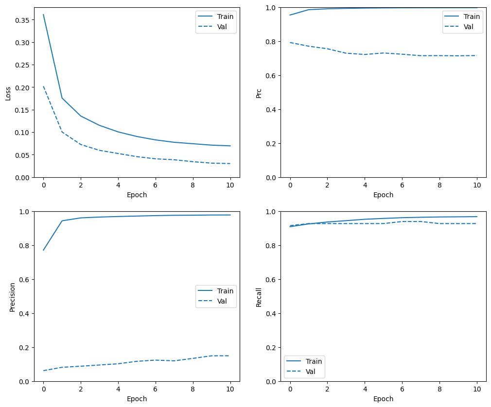
Re-train
Because training is easier on the balanced data, the above training procedure may overfit quickly.
So break up the epochs to give the tf.keras.callbacks.EarlyStopping finer control over when to stop training.
resampled_model = make_model()
resampled_model.load_weights(initial_weights)

# Reset the bias to zero, since this dataset is balanced.
output_layer = resampled_model.layers[-1]
output_layer.bias.assign([0])

resampled_history = resampled_model.fit(
    resampled_ds,
    # These are not real epochs
    steps_per_epoch=20,
    epochs=10*EPOCHS,
    callbacks=[early_stopping()],
    validation_data=(val_ds))
Epoch 1/1000
20/20 ━━━━━━━━━━━━━━━━━━━━ 6s 146ms/step - Brier score: 0.0854 - accuracy: 0.8656 - auc: 0.9253 - cross entropy: 0.2545 - fn: 3317.8572 - fp: 6401.5239 - loss: 0.7612 - prc: 0.6796 - precision: 0.5317 - recall: 0.6887 - tn: 50418.2383 - tp: 7861.8569 - val_Brier score: 0.2768 - val_accuracy: 0.4990 - val_auc: 0.9432 - val_cross entropy: 0.7582 - val_fn: 3.0000 - val_fp: 22829.0000 - val_loss: 0.7582 - val_prc: 0.3111 - val_precision: 0.0034 - val_recall: 0.9634 - val_tn: 22658.0000 - val_tp: 79.0000
Epoch 2/1000
20/20 ━━━━━━━━━━━━━━━━━━━━ 1s 28ms/step - Brier score: 0.1998 - accuracy: 0.6788 - auc: 0.8035 - cross entropy: 0.5771 - fn: 1924.4762 - fp: 5174.4287 - loss: 0.5771 - prc: 0.8480 - precision: 0.6421 - recall: 0.8240 - tn: 5957.5239 - tp: 9374.0479 - val_Brier score: 0.2384 - val_accuracy: 0.6159 - val_auc: 0.9514 - val_cross entropy: 0.6743 - val_fn: 3.0000 - val_fp: 17501.0000 - val_loss: 0.6743 - val_prc: 0.6435 - val_precision: 0.0045 - val_recall: 0.9634 - val_tn: 27986.0000 - val_tp: 79.0000
Epoch 3/1000
20/20 ━━━━━━━━━━━━━━━━━━━━ 1s 28ms/step - Brier score: 0.1759 - accuracy: 0.7240 - auc: 0.8564 - cross entropy: 0.5143 - fn: 1575.7620 - fp: 4516.0952 - loss: 0.5143 - prc: 0.8870 - precision: 0.6754 - recall: 0.8579 - tn: 6751.8569 - tp: 9586.7617 - val_Brier score: 0.2005 - val_accuracy: 0.7314 - val_auc: 0.9561 - val_cross entropy: 0.5917 - val_fn: 4.0000 - val_fp: 12234.0000 - val_loss: 0.5917 - val_prc: 0.7039 - val_precision: 0.0063 - val_recall: 0.9512 - val_tn: 33253.0000 - val_tp: 78.0000
Epoch 4/1000
20/20 ━━━━━━━━━━━━━━━━━━━━ 1s 28ms/step - Brier score: 0.1528 - accuracy: 0.7666 - auc: 0.8872 - cross entropy: 0.4537 - fn: 1515.7620 - fp: 3679.7620 - loss: 0.4537 - prc: 0.9127 - precision: 0.7236 - recall: 0.8662 - tn: 7503.4761 - tp: 9731.4766 - val_Brier score: 0.1704 - val_accuracy: 0.8147 - val_auc: 0.9601 - val_cross entropy: 0.5256 - val_fn: 5.0000 - val_fp: 8439.0000 - val_loss: 0.5256 - val_prc: 0.7351 - val_precision: 0.0090 - val_recall: 0.9390 - val_tn: 37048.0000 - val_tp: 77.0000
Epoch 5/1000
20/20 ━━━━━━━━━━━━━━━━━━━━ 0s 26ms/step - Brier score: 0.1399 - accuracy: 0.7916 - auc: 0.9011 - cross entropy: 0.4172 - fn: 1509.0476 - fp: 3090.4285 - loss: 0.4172 - prc: 0.9263 - precision: 0.7574 - recall: 0.8647 - tn: 8035.0000 - tp: 9796.0000 - val_Brier score: 0.1466 - val_accuracy: 0.8680 - val_auc: 0.9637 - val_cross entropy: 0.4722 - val_fn: 5.0000 - val_fp: 6008.0000 - val_loss: 0.4722 - val_prc: 0.7597 - val_precision: 0.0127 - val_recall: 0.9390 - val_tn: 39479.0000 - val_tp: 77.0000
Epoch 6/1000
20/20 ━━━━━━━━━━━━━━━━━━━━ 0s 24ms/step - Brier score: 0.1283 - accuracy: 0.8136 - auc: 0.9144 - cross entropy: 0.3884 - fn: 1419.9048 - fp: 2720.1904 - loss: 0.3884 - prc: 0.9374 - precision: 0.7837 - recall: 0.8757 - tn: 8316.5713 - tp: 9973.8096 - val_Brier score: 0.1263 - val_accuracy: 0.9040 - val_auc: 0.9668 - val_cross entropy: 0.4258 - val_fn: 5.0000 - val_fp: 4368.0000 - val_loss: 0.4258 - val_prc: 0.7771 - val_precision: 0.0173 - val_recall: 0.9390 - val_tn: 41119.0000 - val_tp: 77.0000
Epoch 7/1000
20/20 ━━━━━━━━━━━━━━━━━━━━ 0s 24ms/step - Brier score: 0.1164 - accuracy: 0.8351 - auc: 0.9278 - cross entropy: 0.3575 - fn: 1410.5238 - fp: 2263.9524 - loss: 0.3575 - prc: 0.9460 - precision: 0.8105 - recall: 0.8749 - tn: 8921.5713 - tp: 9834.4287 - val_Brier score: 0.1079 - val_accuracy: 0.9311 - val_auc: 0.9695 - val_cross entropy: 0.3819 - val_fn: 5.0000 - val_fp: 3136.0000 - val_loss: 0.3819 - val_prc: 0.7823 - val_precision: 0.0240 - val_recall: 0.9390 - val_tn: 42351.0000 - val_tp: 77.0000
Epoch 8/1000
20/20 ━━━━━━━━━━━━━━━━━━━━ 0s 24ms/step - Brier score: 0.1081 - accuracy: 0.8470 - auc: 0.9345 - cross entropy: 0.3353 - fn: 1414.0952 - fp: 1964.7620 - loss: 0.3353 - prc: 0.9508 - precision: 0.8286 - recall: 0.8740 - tn: 9261.8096 - tp: 9789.8096 - val_Brier score: 0.0926 - val_accuracy: 0.9487 - val_auc: 0.9721 - val_cross entropy: 0.3441 - val_fn: 5.0000 - val_fp: 2334.0000 - val_loss: 0.3441 - val_prc: 0.7887 - val_precision: 0.0319 - val_recall: 0.9390 - val_tn: 43153.0000 - val_tp: 77.0000
Epoch 9/1000
20/20 ━━━━━━━━━━━━━━━━━━━━ 0s 24ms/step - Brier score: 0.0994 - accuracy: 0.8665 - auc: 0.9419 - cross entropy: 0.3134 - fn: 1385.7142 - fp: 1594.3810 - loss: 0.3134 - prc: 0.9564 - precision: 0.8608 - recall: 0.8769 - tn: 9544.9521 - tp: 9905.4287 - val_Brier score: 0.0800 - val_accuracy: 0.9605 - val_auc: 0.9745 - val_cross entropy: 0.3111 - val_fn: 5.0000 - val_fp: 1794.0000 - val_loss: 0.3111 - val_prc: 0.7932 - val_precision: 0.0412 - val_recall: 0.9390 - val_tn: 43693.0000 - val_tp: 77.0000
Epoch 10/1000
20/20 ━━━━━━━━━━━━━━━━━━━━ 0s 23ms/step - Brier score: 0.0932 - accuracy: 0.8743 - auc: 0.9474 - cross entropy: 0.2961 - fn: 1371.6190 - fp: 1409.3810 - loss: 0.2961 - prc: 0.9602 - precision: 0.8727 - recall: 0.8781 - tn: 9730.0000 - tp: 9919.4766 - val_Brier score: 0.0703 - val_accuracy: 0.9667 - val_auc: 0.9773 - val_cross entropy: 0.2844 - val_fn: 5.0000 - val_fp: 1514.0000 - val_loss: 0.2844 - val_prc: 0.7895 - val_precision: 0.0484 - val_recall: 0.9390 - val_tn: 43973.0000 - val_tp: 77.0000
Epoch 11/1000
20/20 ━━━━━━━━━━━━━━━━━━━━ 0s 24ms/step - Brier score: 0.0877 - accuracy: 0.8832 - auc: 0.9520 - cross entropy: 0.2804 - fn: 1342.0000 - fp: 1251.1904 - loss: 0.2804 - prc: 0.9637 - precision: 0.8863 - recall: 0.8798 - tn: 9908.1904 - tp: 9929.0957 - val_Brier score: 0.0620 - val_accuracy: 0.9704 - val_auc: 0.9792 - val_cross entropy: 0.2602 - val_fn: 5.0000 - val_fp: 1345.0000 - val_loss: 0.2602 - val_prc: 0.7840 - val_precision: 0.0541 - val_recall: 0.9390 - val_tn: 44142.0000 - val_tp: 77.0000
Epoch 12/1000
20/20 ━━━━━━━━━━━━━━━━━━━━ 0s 24ms/step - Brier score: 0.0821 - accuracy: 0.8911 - auc: 0.9562 - cross entropy: 0.2644 - fn: 1335.1904 - fp: 1104.5238 - loss: 0.2644 - prc: 0.9665 - precision: 0.8995 - recall: 0.8808 - tn: 10111.1426 - tp: 9879.6191 - val_Brier score: 0.0550 - val_accuracy: 0.9731 - val_auc: 0.9809 - val_cross entropy: 0.2388 - val_fn: 5.0000 - val_fp: 1223.0000 - val_loss: 0.2388 - val_prc: 0.7881 - val_precision: 0.0592 - val_recall: 0.9390 - val_tn: 44264.0000 - val_tp: 77.0000
Epoch 13/1000
20/20 ━━━━━━━━━━━━━━━━━━━━ 0s 24ms/step - Brier score: 0.0786 - accuracy: 0.8973 - auc: 0.9590 - cross entropy: 0.2559 - fn: 1280.6190 - fp: 1007.5714 - loss: 0.2559 - prc: 0.9681 - precision: 0.9063 - recall: 0.8853 - tn: 10273.3809 - tp: 9868.9043 - val_Brier score: 0.0492 - val_accuracy: 0.9750 - val_auc: 0.9816 - val_cross entropy: 0.2201 - val_fn: 5.0000 - val_fp: 1134.0000 - val_loss: 0.2201 - val_prc: 0.7912 - val_precision: 0.0636 - val_recall: 0.9390 - val_tn: 44353.0000 - val_tp: 77.0000
Epoch 14/1000
20/20 ━━━━━━━━━━━━━━━━━━━━ 0s 25ms/step - Brier score: 0.0739 - accuracy: 0.9064 - auc: 0.9633 - cross entropy: 0.2422 - fn: 1233.4762 - fp: 868.5238 - loss: 0.2422 - prc: 0.9717 - precision: 0.9194 - recall: 0.8912 - tn: 10317.9043 - tp: 10010.5713 - val_Brier score: 0.0447 - val_accuracy: 0.9759 - val_auc: 0.9824 - val_cross entropy: 0.2045 - val_fn: 5.0000 - val_fp: 1091.0000 - val_loss: 0.2045 - val_prc: 0.7934 - val_precision: 0.0659 - val_recall: 0.9390 - val_tn: 44396.0000 - val_tp: 77.0000
Epoch 15/1000
20/20 ━━━━━━━━━━━━━━━━━━━━ 0s 24ms/step - Brier score: 0.0731 - accuracy: 0.9042 - auc: 0.9633 - cross entropy: 0.2390 - fn: 1247.2380 - fp: 881.2381 - loss: 0.2390 - prc: 0.9713 - precision: 0.9170 - recall: 0.8877 - tn: 10373.6191 - tp: 9928.3809 - val_Brier score: 0.0412 - val_accuracy: 0.9767 - val_auc: 0.9828 - val_cross entropy: 0.1919 - val_fn: 5.0000 - val_fp: 1059.0000 - val_loss: 0.1919 - val_prc: 0.7955 - val_precision: 0.0678 - val_recall: 0.9390 - val_tn: 44428.0000 - val_tp: 77.0000
Epoch 16/1000
20/20 ━━━━━━━━━━━━━━━━━━━━ 0s 26ms/step - Brier score: 0.0697 - accuracy: 0.9079 - auc: 0.9666 - cross entropy: 0.2300 - fn: 1205.6666 - fp: 856.9524 - loss: 0.2300 - prc: 0.9736 - precision: 0.9208 - recall: 0.8926 - tn: 10364.8574 - tp: 10003.0000 - val_Brier score: 0.0380 - val_accuracy: 0.9775 - val_auc: 0.9833 - val_cross entropy: 0.1800 - val_fn: 5.0000 - val_fp: 1019.0000 - val_loss: 0.1800 - val_prc: 0.7976 - val_precision: 0.0703 - val_recall: 0.9390 - val_tn: 44468.0000 - val_tp: 77.0000
Epoch 17/1000
20/20 ━━━━━━━━━━━━━━━━━━━━ 0s 26ms/step - Brier score: 0.0670 - accuracy: 0.9130 - auc: 0.9688 - cross entropy: 0.2209 - fn: 1197.1428 - fp: 747.4286 - loss: 0.2209 - prc: 0.9753 - precision: 0.9295 - recall: 0.8943 - tn: 10411.0479 - tp: 10074.8574 - val_Brier score: 0.0358 - val_accuracy: 0.9777 - val_auc: 0.9836 - val_cross entropy: 0.1710 - val_fn: 5.0000 - val_fp: 1013.0000 - val_loss: 0.1710 - val_prc: 0.7976 - val_precision: 0.0706 - val_recall: 0.9390 - val_tn: 44474.0000 - val_tp: 77.0000
Epoch 18/1000
20/20 ━━━━━━━━━━━━━━━━━━━━ 0s 26ms/step - Brier score: 0.0657 - accuracy: 0.9141 - auc: 0.9687 - cross entropy: 0.2163 - fn: 1195.1904 - fp: 714.6190 - loss: 0.2163 - prc: 0.9755 - precision: 0.9331 - recall: 0.8919 - tn: 10524.4766 - tp: 9996.1904 - val_Brier score: 0.0340 - val_accuracy: 0.9775 - val_auc: 0.9838 - val_cross entropy: 0.1632 - val_fn: 5.0000 - val_fp: 1022.0000 - val_loss: 0.1632 - val_prc: 0.7981 - val_precision: 0.0701 - val_recall: 0.9390 - val_tn: 44465.0000 - val_tp: 77.0000
Epoch 19/1000
20/20 ━━━━━━━━━━━━━━━━━━━━ 1s 27ms/step - Brier score: 0.0623 - accuracy: 0.9184 - auc: 0.9721 - cross entropy: 0.2066 - fn: 1152.6190 - fp: 673.1905 - loss: 0.2066 - prc: 0.9779 - precision: 0.9370 - recall: 0.8960 - tn: 10617.4287 - tp: 9987.2383 - val_Brier score: 0.0321 - val_accuracy: 0.9777 - val_auc: 0.9842 - val_cross entropy: 0.1556 - val_fn: 5.0000 - val_fp: 1011.0000 - val_loss: 0.1556 - val_prc: 0.7999 - val_precision: 0.0708 - val_recall: 0.9390 - val_tn: 44476.0000 - val_tp: 77.0000
Epoch 20/1000
20/20 ━━━━━━━━━━━━━━━━━━━━ 0s 26ms/step - Brier score: 0.0618 - accuracy: 0.9184 - auc: 0.9728 - cross entropy: 0.2065 - fn: 1139.0952 - fp: 684.5238 - loss: 0.2065 - prc: 0.9777 - precision: 0.9362 - recall: 0.8974 - tn: 10583.5234 - tp: 10023.3330 - val_Brier score: 0.0304 - val_accuracy: 0.9782 - val_auc: 0.9845 - val_cross entropy: 0.1483 - val_fn: 5.0000 - val_fp: 990.0000 - val_loss: 0.1483 - val_prc: 0.8002 - val_precision: 0.0722 - val_recall: 0.9390 - val_tn: 44497.0000 - val_tp: 77.0000
Epoch 21/1000
20/20 ━━━━━━━━━━━━━━━━━━━━ 1s 27ms/step - Brier score: 0.0593 - accuracy: 0.9230 - auc: 0.9749 - cross entropy: 0.1981 - fn: 1089.2380 - fp: 639.9524 - loss: 0.1981 - prc: 0.9791 - precision: 0.9398 - recall: 0.9014 - tn: 10744.6670 - tp: 9956.6191 - val_Brier score: 0.0289 - val_accuracy: 0.9789 - val_auc: 0.9849 - val_cross entropy: 0.1419 - val_fn: 5.0000 - val_fp: 958.0000 - val_loss: 0.1419 - val_prc: 0.8002 - val_precision: 0.0744 - val_recall: 0.9390 - val_tn: 44529.0000 - val_tp: 77.0000
Epoch 22/1000
20/20 ━━━━━━━━━━━━━━━━━━━━ 1s 26ms/step - Brier score: 0.0589 - accuracy: 0.9240 - auc: 0.9752 - cross entropy: 0.1983 - fn: 1054.1904 - fp: 632.2857 - loss: 0.1983 - prc: 0.9794 - precision: 0.9395 - recall: 0.9059 - tn: 10657.0000 - tp: 10087.0000 - val_Brier score: 0.0276 - val_accuracy: 0.9795 - val_auc: 0.9855 - val_cross entropy: 0.1360 - val_fn: 5.0000 - val_fp: 928.0000 - val_loss: 0.1360 - val_prc: 0.8008 - val_precision: 0.0766 - val_recall: 0.9390 - val_tn: 44559.0000 - val_tp: 77.0000
Epoch 23/1000
20/20 ━━━━━━━━━━━━━━━━━━━━ 1s 28ms/step - Brier score: 0.0573 - accuracy: 0.9267 - auc: 0.9764 - cross entropy: 0.1905 - fn: 1066.1428 - fp: 581.2381 - loss: 0.1905 - prc: 0.9805 - precision: 0.9449 - recall: 0.9055 - tn: 10638.0479 - tp: 10145.0479 - val_Brier score: 0.0266 - val_accuracy: 0.9798 - val_auc: 0.9857 - val_cross entropy: 0.1311 - val_fn: 5.0000 - val_fp: 914.0000 - val_loss: 0.1311 - val_prc: 0.8010 - val_precision: 0.0777 - val_recall: 0.9390 - val_tn: 44573.0000 - val_tp: 77.0000
Epoch 24/1000
20/20 ━━━━━━━━━━━━━━━━━━━━ 1s 27ms/step - Brier score: 0.0564 - accuracy: 0.9264 - auc: 0.9770 - cross entropy: 0.1879 - fn: 1040.5238 - fp: 611.6667 - loss: 0.1879 - prc: 0.9811 - precision: 0.9431 - recall: 0.9072 - tn: 10623.2861 - tp: 10155.0000 - val_Brier score: 0.0255 - val_accuracy: 0.9802 - val_auc: 0.9862 - val_cross entropy: 0.1263 - val_fn: 5.0000 - val_fp: 895.0000 - val_loss: 0.1263 - val_prc: 0.7927 - val_precision: 0.0792 - val_recall: 0.9390 - val_tn: 44592.0000 - val_tp: 77.0000
Epoch 25/1000
20/20 ━━━━━━━━━━━━━━━━━━━━ 1s 29ms/step - Brier score: 0.0543 - accuracy: 0.9297 - auc: 0.9786 - cross entropy: 0.1820 - fn: 1029.3810 - fp: 555.0000 - loss: 0.1820 - prc: 0.9819 - precision: 0.9481 - recall: 0.9075 - tn: 10767.4287 - tp: 10078.6670 - val_Brier score: 0.0245 - val_accuracy: 0.9804 - val_auc: 0.9864 - val_cross entropy: 0.1217 - val_fn: 5.0000 - val_fp: 887.0000 - val_loss: 0.1217 - val_prc: 0.7928 - val_precision: 0.0799 - val_recall: 0.9390 - val_tn: 44600.0000 - val_tp: 77.0000
Epoch 26/1000
20/20 ━━━━━━━━━━━━━━━━━━━━ 1s 27ms/step - Brier score: 0.0540 - accuracy: 0.9308 - auc: 0.9790 - cross entropy: 0.1803 - fn: 1024.8572 - fp: 514.5714 - loss: 0.1803 - prc: 0.9827 - precision: 0.9510 - recall: 0.9082 - tn: 10685.9043 - tp: 10205.1426 - val_Brier score: 0.0237 - val_accuracy: 0.9807 - val_auc: 0.9864 - val_cross entropy: 0.1180 - val_fn: 5.0000 - val_fp: 874.0000 - val_loss: 0.1180 - val_prc: 0.7845 - val_precision: 0.0810 - val_recall: 0.9390 - val_tn: 44613.0000 - val_tp: 77.0000
Epoch 27/1000
20/20 ━━━━━━━━━━━━━━━━━━━━ 1s 26ms/step - Brier score: 0.0528 - accuracy: 0.9310 - auc: 0.9801 - cross entropy: 0.1770 - fn: 1002.4762 - fp: 533.0952 - loss: 0.1770 - prc: 0.9832 - precision: 0.9501 - recall: 0.9103 - tn: 10691.4766 - tp: 10203.4287 - val_Brier score: 0.0230 - val_accuracy: 0.9811 - val_auc: 0.9867 - val_cross entropy: 0.1144 - val_fn: 5.0000 - val_fp: 858.0000 - val_loss: 0.1144 - val_prc: 0.7843 - val_precision: 0.0824 - val_recall: 0.9390 - val_tn: 44629.0000 - val_tp: 77.0000
Epoch 28/1000
20/20 ━━━━━━━━━━━━━━━━━━━━ 1s 26ms/step - Brier score: 0.0530 - accuracy: 0.9300 - auc: 0.9802 - cross entropy: 0.1762 - fn: 992.1905 - fp: 547.8095 - loss: 0.1762 - prc: 0.9832 - precision: 0.9467 - recall: 0.9107 - tn: 10725.5234 - tp: 10164.9521 - val_Brier score: 0.0222 - val_accuracy: 0.9815 - val_auc: 0.9870 - val_cross entropy: 0.1106 - val_fn: 5.0000 - val_fp: 839.0000 - val_loss: 0.1106 - val_prc: 0.7847 - val_precision: 0.0841 - val_recall: 0.9390 - val_tn: 44648.0000 - val_tp: 77.0000
Epoch 29/1000
20/20 ━━━━━━━━━━━━━━━━━━━━ 0s 24ms/step - Brier score: 0.0503 - accuracy: 0.9352 - auc: 0.9820 - cross entropy: 0.1677 - fn: 971.4762 - fp: 486.4762 - loss: 0.1677 - prc: 0.9849 - precision: 0.9542 - recall: 0.9146 - tn: 10711.7617 - tp: 10260.7617 - val_Brier score: 0.0219 - val_accuracy: 0.9813 - val_auc: 0.9866 - val_cross entropy: 0.1085 - val_fn: 5.0000 - val_fp: 846.0000 - val_loss: 0.1085 - val_prc: 0.7853 - val_precision: 0.0834 - val_recall: 0.9390 - val_tn: 44641.0000 - val_tp: 77.0000
Epoch 30/1000
20/20 ━━━━━━━━━━━━━━━━━━━━ 0s 24ms/step - Brier score: 0.0503 - accuracy: 0.9357 - auc: 0.9817 - cross entropy: 0.1684 - fn: 944.7143 - fp: 492.0000 - loss: 0.1684 - prc: 0.9845 - precision: 0.9541 - recall: 0.9152 - tn: 10743.7139 - tp: 10250.0479 - val_Brier score: 0.0214 - val_accuracy: 0.9813 - val_auc: 0.9868 - val_cross entropy: 0.1059 - val_fn: 5.0000 - val_fp: 849.0000 - val_loss: 0.1059 - val_prc: 0.7861 - val_precision: 0.0832 - val_recall: 0.9390 - val_tn: 44638.0000 - val_tp: 77.0000
Epoch 31/1000
20/20 ━━━━━━━━━━━━━━━━━━━━ 0s 24ms/step - Brier score: 0.0491 - accuracy: 0.9375 - auc: 0.9828 - cross entropy: 0.1663 - fn: 953.2381 - fp: 452.3810 - loss: 0.1663 - prc: 0.9852 - precision: 0.9581 - recall: 0.9148 - tn: 10786.8096 - tp: 10238.0479 - val_Brier score: 0.0209 - val_accuracy: 0.9814 - val_auc: 0.9870 - val_cross entropy: 0.1031 - val_fn: 5.0000 - val_fp: 844.0000 - val_loss: 0.1031 - val_prc: 0.7774 - val_precision: 0.0836 - val_recall: 0.9390 - val_tn: 44643.0000 - val_tp: 77.0000
Epoch 32/1000
20/20 ━━━━━━━━━━━━━━━━━━━━ 0s 25ms/step - Brier score: 0.0487 - accuracy: 0.9377 - auc: 0.9836 - cross entropy: 0.1640 - fn: 953.1905 - fp: 451.4286 - loss: 0.1640 - prc: 0.9856 - precision: 0.9572 - recall: 0.9150 - tn: 10828.9043 - tp: 10196.9521 - val_Brier score: 0.0206 - val_accuracy: 0.9813 - val_auc: 0.9872 - val_cross entropy: 0.1010 - val_fn: 5.0000 - val_fp: 849.0000 - val_loss: 0.1010 - val_prc: 0.7774 - val_precision: 0.0832 - val_recall: 0.9390 - val_tn: 44638.0000 - val_tp: 77.0000
Epoch 33/1000
20/20 ━━━━━━━━━━━━━━━━━━━━ 0s 25ms/step - Brier score: 0.0479 - accuracy: 0.9378 - auc: 0.9836 - cross entropy: 0.1604 - fn: 931.0476 - fp: 467.4762 - loss: 0.1604 - prc: 0.9863 - precision: 0.9565 - recall: 0.9177 - tn: 10702.9521 - tp: 10329.0000 - val_Brier score: 0.0203 - val_accuracy: 0.9813 - val_auc: 0.9874 - val_cross entropy: 0.0994 - val_fn: 5.0000 - val_fp: 849.0000 - val_loss: 0.0994 - val_prc: 0.7777 - val_precision: 0.0832 - val_recall: 0.9390 - val_tn: 44638.0000 - val_tp: 77.0000
Epoch 33: early stopping
Restoring model weights from the end of the best epoch: 23.
Re-check training history
plot_metrics(resampled_history)
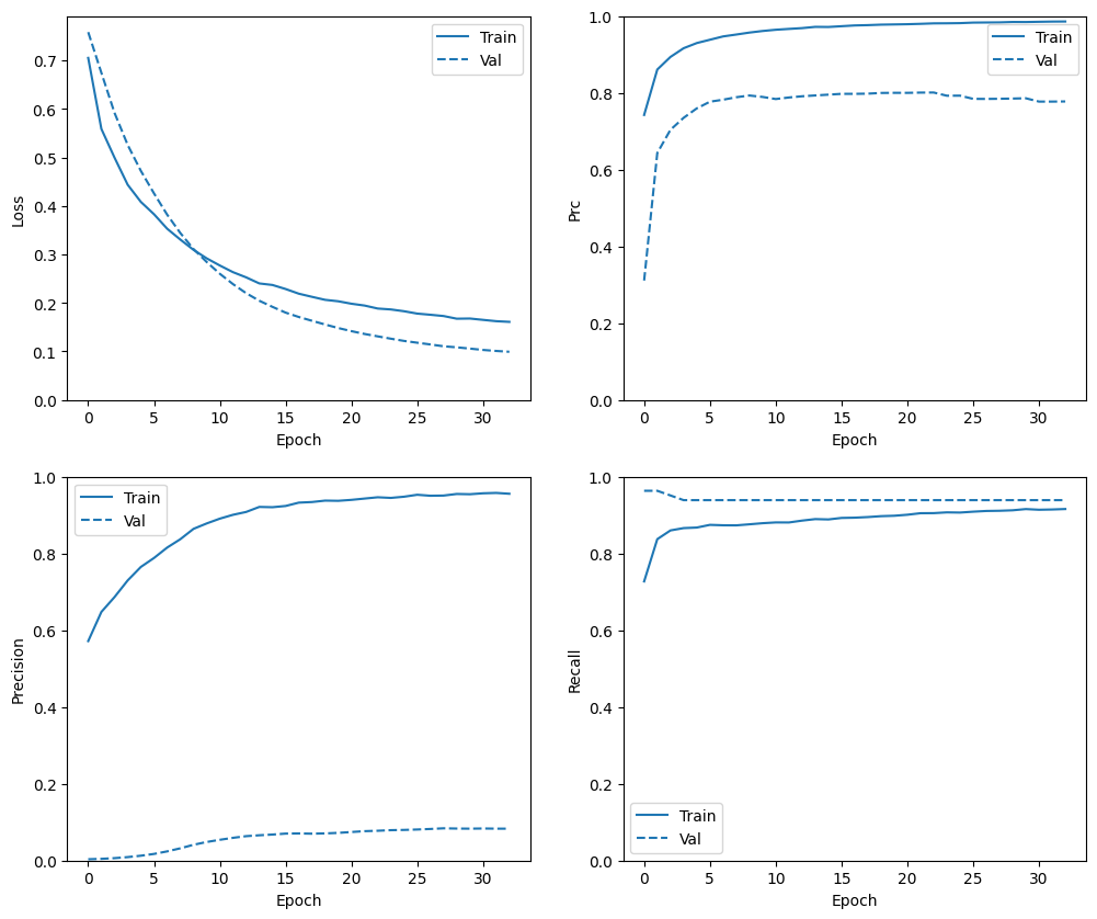
Evaluate metrics
train_predictions_resampled = resampled_model.predict(train_features, batch_size=BATCH_SIZE)
test_predictions_resampled = resampled_model.predict(test_features, batch_size=BATCH_SIZE)
90/90 ━━━━━━━━━━━━━━━━━━━━ 0s 2ms/step
28/28 ━━━━━━━━━━━━━━━━━━━━ 0s 3ms/step
resampled_results = resampled_model.evaluate(test_features, test_labels,
                                             batch_size=BATCH_SIZE, verbose=0)
for name, value in zip(resampled_model.metrics_names, resampled_results):
  print(name, ': ', value)
print()
plot_cm(test_labels, test_predictions_resampled)
loss :  0.129319429397583
compile_metrics :  0.129319429397583

Legitimate Transactions Detected (True Negatives):  55717
Legitimate Transactions Incorrectly Detected (False Positives):  1143
Fraudulent Transactions Missed (False Negatives):  9
Fraudulent Transactions Detected (True Positives):  93
Total Fraudulent Transactions:  102

Plot the ROC
plot_roc("Train Baseline", train_labels, train_predictions_baseline, color=colors[0])
plot_roc("Test Baseline", test_labels, test_predictions_baseline, color=colors[0], linestyle='--')
plot_roc("Train Weighted", train_labels, train_predictions_weighted, color=colors[1])
plot_roc("Test Weighted", test_labels, test_predictions_weighted, color=colors[1], linestyle='--')
plot_roc("Train Resampled", train_labels, train_predictions_resampled, color=colors[2])
plot_roc("Test Resampled", test_labels, test_predictions_resampled, color=colors[2], linestyle='--')
plt.legend(loc='lower right');
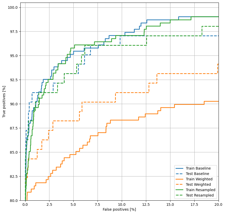
Plot the AUPRC
plot_prc("Train Baseline", train_labels, train_predictions_baseline, color=colors[0])
plot_prc("Test Baseline", test_labels, test_predictions_baseline, color=colors[0], linestyle='--')

plot_prc("Train Weighted", train_labels, train_predictions_weighted, color=colors[1])
plot_prc("Test Weighted", test_labels, test_predictions_weighted, color=colors[1], linestyle='--')

plot_prc("Train Resampled", train_labels, train_predictions_resampled, color=colors[2])
plot_prc("Test Resampled", test_labels, test_predictions_resampled, color=colors[2], linestyle='--')
plt.legend(loc='lower right');
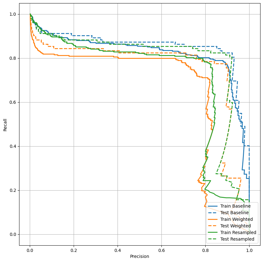
Applying this tutorial to your problem
Imbalanced data classification is an inherently difficult task since there are so few samples to learn from. You should always start with the data first and do your best to collect as many samples as possible and give substantial thought to what features may be relevant so the model can get the most out of your minority class. At some point your model may struggle to improve and yield the results you want, so it is important to keep in mind the context of your problem and the trade offs between different types of errors.