Transfer learning for video classification with MoViNet

View on TensorFlow.org

Run in Google Colab

View source on GitHub

Download notebook

MoViNets (Mobile Video Networks) provide a family of efficient video classification models, supporting inference on streaming video. In this tutorial, you will use a pre-trained MoViNet model to classify videos, specifically for an action recognition task, from the UCF101 dataset. A pre-trained model is a saved network that was previously trained on a larger dataset. You can find more details about MoViNets in the MoViNets: Mobile Video Networks for Efficient Video Recognition paper by Kondratyuk, D. et al. (2021). In this tutorial, you will:

• Learn how to download a pre-trained MoViNet model
• Create a new model using a pre-trained model with a new classifier by freezing the convolutional base of the MoViNet model
• Replace the classifier head with the number of labels of a new dataset
• Perform transfer learning on the UCF101 dataset

The model downloaded in this tutorial is from official/projects/movinet. This repository contains a collection of MoViNet models that TF Hub uses in the TensorFlow 2 SavedModel format.

This transfer learning tutorial is the third part in a series of TensorFlow video tutorials. Here are the other three tutorials:

• Load video data: This tutorial explains much of the code used in this document; in particular, how to preprocess and load data through the FrameGenerator class is explained in more detail.
• Build a 3D CNN model for video classification. Note that this tutorial uses a (2+1)D CNN that decomposes the spatial and temporal aspects of 3D data; if you are using volumetric data such as an MRI scan, consider using a 3D CNN instead of a (2+1)D CNN.
• MoViNet for streaming action recognition: Get familiar with the MoViNet models that are available on TF Hub.

Setup

Begin by installing and importing some necessary libraries, including: remotezip to inspect the contents of a ZIP file, tqdm to use a progress bar, OpenCV to process video files (ensure that opencv-python and opencv-python-headless are the same version), and TensorFlow models (tf-models-official) to download the pre-trained MoViNet model. The TensorFlow models package are a collection of models that use TensorFlow’s high-level APIs.

pip install remotezip tqdm opencv-python==4.5.2.52 opencv-python-headless==4.5.2.52 tf-models-official

import tqdm
import random
import pathlib
import itertools
import collections

import cv2
import numpy as np
import remotezip as rz
import seaborn as sns
import matplotlib.pyplot as plt

import keras
import tensorflow as tf
import tensorflow_hub as hub
from tensorflow.keras import layers
from tensorflow.keras.optimizers import Adam
from tensorflow.keras.losses import SparseCategoricalCrossentropy

# Import the MoViNet model from TensorFlow Models (tf-models-official) for the MoViNet model
from official.projects.movinet.modeling import movinet
from official.projects.movinet.modeling import movinet_model

2023-10-27 04:37:58.081880: E tensorflow/compiler/xla/stream_executor/cuda/cuda_dnn.cc:9342] Unable to register cuDNN factory: Attempting to register factory for plugin cuDNN when one has already been registered
2023-10-27 04:37:58.081941: E tensorflow/compiler/xla/stream_executor/cuda/cuda_fft.cc:609] Unable to register cuFFT factory: Attempting to register factory for plugin cuFFT when one has already been registered
2023-10-27 04:37:58.082006: E tensorflow/compiler/xla/stream_executor/cuda/cuda_blas.cc:1518] Unable to register cuBLAS factory: Attempting to register factory for plugin cuBLAS when one has already been registered

Load data

The hidden cell below defines helper functions to download a slice of data from the UCF-101 dataset, and load it into a tf.data.Dataset. The Loading video data tutorial provides a detailed walkthrough of this code.

The FrameGenerator class at the end of the hidden block is the most important utility here. It creates an iterable object that can feed data into the TensorFlow data pipeline. Specifically, this class contains a Python generator that loads the video frames along with its encoded label. The generator (__call__) function yields the frame array produced by frames_from_video_file and a one-hot encoded vector of the label associated with the set of frames.

def list_files_per_class(zip_url):
  """
    List the files in each class of the dataset given the zip URL.

    Args:
      zip_url: URL from which the files can be unzipped. 

    Return:
      files: List of files in each of the classes.
  """
  files = []
  with rz.RemoteZip(URL) as zip:
    for zip_info in zip.infolist():
      files.append(zip_info.filename)
  return files

def get_class(fname):
  """
    Retrieve the name of the class given a filename.

    Args:
      fname: Name of the file in the UCF101 dataset.

    Return:
      Class that the file belongs to.
  """
  return fname.split('_')[-3]

def get_files_per_class(files):
  """
    Retrieve the files that belong to each class. 

    Args:
      files: List of files in the dataset.

    Return:
      Dictionary of class names (key) and files (values).
  """
  files_for_class = collections.defaultdict(list)
  for fname in files:
    class_name = get_class(fname)
    files_for_class[class_name].append(fname)
  return files_for_class

def download_from_zip(zip_url, to_dir, file_names):
  """
    Download the contents of the zip file from the zip URL.

    Args:
      zip_url: Zip URL containing data.
      to_dir: Directory to download data to.
      file_names: Names of files to download.
  """
  with rz.RemoteZip(zip_url) as zip:
    for fn in tqdm.tqdm(file_names):
      class_name = get_class(fn)
      zip.extract(fn, str(to_dir / class_name))
      unzipped_file = to_dir / class_name / fn

      fn = pathlib.Path(fn).parts[-1]
      output_file = to_dir / class_name / fn
      unzipped_file.rename(output_file,)

def split_class_lists(files_for_class, count):
  """
    Returns the list of files belonging to a subset of data as well as the remainder of
    files that need to be downloaded.

    Args:
      files_for_class: Files belonging to a particular class of data.
      count: Number of files to download.

    Return:
      split_files: Files belonging to the subset of data.
      remainder: Dictionary of the remainder of files that need to be downloaded.
  """
  split_files = []
  remainder = {}
  for cls in files_for_class:
    split_files.extend(files_for_class[cls][:count])
    remainder[cls] = files_for_class[cls][count:]
  return split_files, remainder

def download_ufc_101_subset(zip_url, num_classes, splits, download_dir):
  """
    Download a subset of the UFC101 dataset and split them into various parts, such as
    training, validation, and test. 

    Args:
      zip_url: Zip URL containing data.
      num_classes: Number of labels.
      splits: Dictionary specifying the training, validation, test, etc. (key) division of data 
              (value is number of files per split).
      download_dir: Directory to download data to.

    Return:
      dir: Posix path of the resulting directories containing the splits of data.
  """
  files = list_files_per_class(zip_url)
  for f in files:
    tokens = f.split('/')
    if len(tokens) <= 2:
      files.remove(f) # Remove that item from the list if it does not have a filename

  files_for_class = get_files_per_class(files)

  classes = list(files_for_class.keys())[:num_classes]

  for cls in classes:
    new_files_for_class = files_for_class[cls]
    random.shuffle(new_files_for_class)
    files_for_class[cls] = new_files_for_class

  # Only use the number of classes you want in the dictionary
  files_for_class = {x: files_for_class[x] for x in list(files_for_class)[:num_classes]}

  dirs = {}
  for split_name, split_count in splits.items():
    print(split_name, ":")
    split_dir = download_dir / split_name
    split_files, files_for_class = split_class_lists(files_for_class, split_count)
    download_from_zip(zip_url, split_dir, split_files)
    dirs[split_name] = split_dir

  return dirs

def format_frames(frame, output_size):
  """
    Pad and resize an image from a video.

    Args:
      frame: Image that needs to resized and padded. 
      output_size: Pixel size of the output frame image.

    Return:
      Formatted frame with padding of specified output size.
  """
  frame = tf.image.convert_image_dtype(frame, tf.float32)
  frame = tf.image.resize_with_pad(frame, *output_size)
  return frame

def frames_from_video_file(video_path, n_frames, output_size = (224,224), frame_step = 15):
  """
    Creates frames from each video file present for each category.

    Args:
      video_path: File path to the video.
      n_frames: Number of frames to be created per video file.
      output_size: Pixel size of the output frame image.

    Return:
      An NumPy array of frames in the shape of (n_frames, height, width, channels).
  """
  # Read each video frame by frame
  result = []
  src = cv2.VideoCapture(str(video_path))  

  video_length = src.get(cv2.CAP_PROP_FRAME_COUNT)

  need_length = 1 + (n_frames - 1) * frame_step

  if need_length > video_length:
    start = 0
  else:
    max_start = video_length - need_length
    start = random.randint(0, max_start + 1)

  src.set(cv2.CAP_PROP_POS_FRAMES, start)
  # ret is a boolean indicating whether read was successful, frame is the image itself
  ret, frame = src.read()
  result.append(format_frames(frame, output_size))

  for _ in range(n_frames - 1):
    for _ in range(frame_step):
      ret, frame = src.read()
    if ret:
      frame = format_frames(frame, output_size)
      result.append(frame)
    else:
      result.append(np.zeros_like(result[0]))
  src.release()
  result = np.array(result)[..., [2, 1, 0]]

  return result

class FrameGenerator:
  def __init__(self, path, n_frames, training = False):
    """ Returns a set of frames with their associated label. 

      Args:
        path: Video file paths.
        n_frames: Number of frames. 
        training: Boolean to determine if training dataset is being created.
    """
    self.path = path
    self.n_frames = n_frames
    self.training = training
    self.class_names = sorted(set(p.name for p in self.path.iterdir() if p.is_dir()))
    self.class_ids_for_name = dict((name, idx) for idx, name in enumerate(self.class_names))

  def get_files_and_class_names(self):
    video_paths = list(self.path.glob('*/*.avi'))
    classes = [p.parent.name for p in video_paths] 
    return video_paths, classes

  def __call__(self):
    video_paths, classes = self.get_files_and_class_names()

    pairs = list(zip(video_paths, classes))

    if self.training:
      random.shuffle(pairs)

    for path, name in pairs:
      video_frames = frames_from_video_file(path, self.n_frames) 
      label = self.class_ids_for_name[name] # Encode labels
      yield video_frames, label

URL = 'https://storage.googleapis.com/thumos14_files/UCF101_videos.zip'
download_dir = pathlib.Path('./UCF101_subset/')
subset_paths = download_ufc_101_subset(URL, 
                        num_classes = 10, 
                        splits = {"train": 30, "test": 20}, 
                        download_dir = download_dir)

train :
100%|██████████| 300/300 [00:28<00:00, 10.68it/s]
test :
100%|██████████| 200/200 [00:18<00:00, 10.70it/s]

Create the training and test datasets:

batch_size = 8
num_frames = 8

output_signature = (tf.TensorSpec(shape = (None, None, None, 3), dtype = tf.float32),
                    tf.TensorSpec(shape = (), dtype = tf.int16))

train_ds = tf.data.Dataset.from_generator(FrameGenerator(subset_paths['train'], num_frames, training = True),
                                          output_signature = output_signature)
train_ds = train_ds.batch(batch_size)

test_ds = tf.data.Dataset.from_generator(FrameGenerator(subset_paths['test'], num_frames),
                                         output_signature = output_signature)
test_ds = test_ds.batch(batch_size)

2023-10-27 04:38:48.976576: W tensorflow/core/common_runtime/gpu/gpu_device.cc:2211] Cannot dlopen some GPU libraries. Please make sure the missing libraries mentioned above are installed properly if you would like to use GPU. Follow the guide at https://www.tensorflow.org/install/gpu for how to download and setup the required libraries for your platform.
Skipping registering GPU devices...

The labels generated here represent the encoding of the classes. For instance, 'ApplyEyeMakeup' is mapped to the integer Take a look at the labels of the training data to ensure that the dataset has been sufficiently shuffled.

for frames, labels in train_ds.take(10):
  print(labels)

tf.Tensor([4 6 7 8 2 4 6 4], shape=(8,), dtype=int16)
tf.Tensor([6 7 7 2 9 2 7 6], shape=(8,), dtype=int16)
tf.Tensor([9 1 1 0 2 3 2 8], shape=(8,), dtype=int16)
tf.Tensor([2 5 6 7 5 8 0 6], shape=(8,), dtype=int16)
tf.Tensor([8 4 2 3 0 5 9 3], shape=(8,), dtype=int16)
tf.Tensor([1 7 3 1 3 1 4 1], shape=(8,), dtype=int16)
tf.Tensor([6 1 7 8 0 6 5 1], shape=(8,), dtype=int16)
tf.Tensor([6 0 7 6 1 8 0 1], shape=(8,), dtype=int16)
tf.Tensor([9 6 7 4 5 3 6 0], shape=(8,), dtype=int16)
tf.Tensor([4 6 4 2 0 1 4 3], shape=(8,), dtype=int16)

Take a look at the shape of the data.

print(f"Shape: {frames.shape}")
print(f"Label: {labels.shape}")

Shape: (8, 8, 224, 224, 3)
Label: (8,)

What are MoViNets?

As mentioned previously, MoViNets are video classification models used for streaming video or online inference in tasks, such as action recognition. Consider using MoViNets to classify your video data for action recognition.

A 2D frame based classifier is efficient and simple to run over whole videos, or streaming one frame at a time. Because they can't take temporal context into account they have limited accuracy and may give inconsistent outputs from frame to frame.

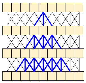
A simple 3D CNN uses bidirectional temporal context which can increase accuracy and temporal consistency. These networks may require more resources and because they look into the future they can't be used for streaming data.

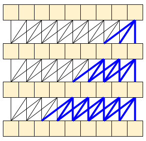
The MoViNet architecture uses 3D convolutions that are "causal" along the time axis (like layers.Conv1D with padding="causal"). This gives some of the advantages of both approaches, mainly it allow for efficient streaming.

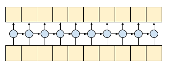
Causal convolution ensures that the output at time t is computed using only inputs up to time t. To demonstrate how this can make streaming more efficient, start with a simpler example you may be familiar with: an RNN. The RNN passes state forward through time:

gru = layers.GRU(units=4, return_sequences=True, return_state=True)

inputs = tf.random.normal(shape=[1, 10, 8]) # (batch, sequence, channels)

result, state = gru(inputs) # Run it all at once

By setting the RNN's return_sequences=True argument you ask it to return the state at the end of the computation. This allows you to pause and then continue where you left off, to get exactly the same result:

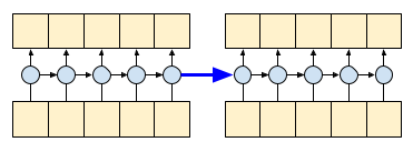
first_half, state = gru(inputs[:, :5, :])   # run the first half, and capture the state
second_half, _ = gru(inputs[:,5:, :], initial_state=state)  # Use the state to continue where you left off.

print(np.allclose(result[:, :5,:], first_half))
print(np.allclose(result[:, 5:,:], second_half))

True
True

Causal convolutions can be used the same way, if handled with care. This technique was used in the Fast Wavenet Generation Algorithm by Le Paine et al. In the MoVinet paper, the state is referred to as the "Stream Buffer".

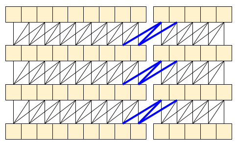
By passing this little bit of state forward, you can avoid recalculating the whole receptive field that shown above.

Download a pre-trained MoViNet model

In this section, you will:

1. You can create a MoViNet model using the open source code provided in official/projects/movinet from TensorFlow models.
2. Load the pretrained weights.
3. Freeze the convolutional base, or all other layers except the final classifier head, to speed up fine-tuning.

To build the model, you can start with the a0 configuration because it is the fastest to train when benchmarked against other models. Check out the available MoViNet models on TensorFlow Model Garden to find what might work for your use case.

model_id = 'a0'
resolution = 224

tf.keras.backend.clear_session()

backbone = movinet.Movinet(model_id=model_id)
backbone.trainable = False

# Set num_classes=600 to load the pre-trained weights from the original model
model = movinet_model.MovinetClassifier(backbone=backbone, num_classes=600)
model.build([None, None, None, None, 3])

# Load pre-trained weights
!wget https://storage.googleapis.com/tf_model_garden/vision/movinet/movinet_a0_base.tar.gz -O movinet_a0_base.tar.gz -q
!tar -xvf movinet_a0_base.tar.gz

checkpoint_dir = f'movinet_{model_id}_base'
checkpoint_path = tf.train.latest_checkpoint(checkpoint_dir)
checkpoint = tf.train.Checkpoint(model=model)
status = checkpoint.restore(checkpoint_path)
status.assert_existing_objects_matched()

movinet_a0_base/
movinet_a0_base/checkpoint
movinet_a0_base/ckpt-1.data-00000-of-00001
movinet_a0_base/ckpt-1.index
<tensorflow.python.checkpoint.checkpoint.CheckpointLoadStatus at 0x7f60fafaafa0>

To build a classifier, create a function that takes the backbone and the number of classes in a dataset. The build_classifier function will take the backbone and the number of classes in a dataset to build the classifier. In this case, the new classifier will take a num_classes outputs (10 classes for this subset of UCF101).

def build_classifier(batch_size, num_frames, resolution, backbone, num_classes):
  """Builds a classifier on top of a backbone model."""
  model = movinet_model.MovinetClassifier(
      backbone=backbone,
      num_classes=num_classes)
  model.build([batch_size, num_frames, resolution, resolution, 3])

  return model

model = build_classifier(batch_size, num_frames, resolution, backbone, 10)

For this tutorial, choose the tf.keras.optimizers.Adam optimizer and the tf.keras.losses.SparseCategoricalCrossentropy loss function. Use the metrics argument to the view the accuracy of the model performance at every step.

num_epochs = 2

loss_obj = tf.keras.losses.SparseCategoricalCrossentropy(from_logits=True)

optimizer = tf.keras.optimizers.Adam(learning_rate = 0.001)

model.compile(loss=loss_obj, optimizer=optimizer, metrics=['accuracy'])

Train the model. After two epochs, observe a low loss with high accuracy for both the training and test sets.

results = model.fit(train_ds,
                    validation_data=test_ds,
                    epochs=num_epochs,
                    validation_freq=1,
                    verbose=1)

Epoch 1/2
2023-10-27 04:39:16.353252: E ./tensorflow/compiler/xla/stream_executor/stream_executor_internal.h:124] SetPriority unimplemented for this stream.
2023-10-27 04:39:16.498099: E ./tensorflow/compiler/xla/stream_executor/stream_executor_internal.h:124] SetPriority unimplemented for this stream.
38/38 [==============================] - 765s 20s/step - loss: 0.9414 - accuracy: 0.7800 - val_loss: 0.2396 - val_accuracy: 0.9450
Epoch 2/2
38/38 [==============================] - 748s 20s/step - loss: 0.1297 - accuracy: 0.9633 - val_loss: 0.1200 - val_accuracy: 0.9750

Evaluate the model

The model achieved high accuracy on the training dataset. Next, use Keras Model.evaluate to evaluate it on the test set.

model.evaluate(test_ds, return_dict=True)

25/25 [==============================] - 295s 12s/step - loss: 0.1135 - accuracy: 0.9700
{'loss': 0.11347560584545135, 'accuracy': 0.9700000286102295}

To visualize model performance further, use a confusion matrix. The confusion matrix allows you to assess the performance of the classification model beyond accuracy. To build the confusion matrix for this multi-class classification problem, get the actual values in the test set and the predicted values.

def get_actual_predicted_labels(dataset):
  """
    Create a list of actual ground truth values and the predictions from the model.

    Args:
      dataset: An iterable data structure, such as a TensorFlow Dataset, with features and labels.

    Return:
      Ground truth and predicted values for a particular dataset.
  """
  actual = [labels for _, labels in dataset.unbatch()]
  predicted = model.predict(dataset)

  actual = tf.stack(actual, axis=0)
  predicted = tf.concat(predicted, axis=0)
  predicted = tf.argmax(predicted, axis=1)

  return actual, predicted

def plot_confusion_matrix(actual, predicted, labels, ds_type):
  cm = tf.math.confusion_matrix(actual, predicted)
  ax = sns.heatmap(cm, annot=True, fmt='g')
  sns.set(rc={'figure.figsize':(12, 12)})
  sns.set(font_scale=1.4)
  ax.set_title('Confusion matrix of action recognition for ' + ds_type)
  ax.set_xlabel('Predicted Action')
  ax.set_ylabel('Actual Action')
  plt.xticks(rotation=90)
  plt.yticks(rotation=0)
  ax.xaxis.set_ticklabels(labels)
  ax.yaxis.set_ticklabels(labels)

fg = FrameGenerator(subset_paths['train'], num_frames, training = True)
label_names = list(fg.class_ids_for_name.keys())

actual, predicted = get_actual_predicted_labels(test_ds)
plot_confusion_matrix(actual, predicted, label_names, 'test')

25/25 [==============================] - 298s 12s/step

Next steps

Now that you have some familiarity with the MoViNet model and how to leverage various TensorFlow APIs (for example, for transfer learning), try using the code in this tutorial with your own dataset. The data does not have to be limited to video data. Volumetric data, such as MRI scans, can also be used with 3D CNNs. The NUSDAT and IMH datasets mentioned in Brain MRI-based 3D Convolutional Neural Networks for Classification of Schizophrenia and Controls could be two such sources for MRI data.

In particular, using the FrameGenerator class used in this tutorial and the other video data and classification tutorials will help you load data into your models.

To learn more about working with video data in TensorFlow, check out the following tutorials:

• Load video data
• Build a 3D CNN model for video classification
• MoViNet for streaming action recognition