|
|
|
 View source on GitHub View source on GitHub
|
|
This tutorial demonstrates how to build and train a conditional generative adversarial network (cGAN) called pix2pix that learns a mapping from input images to output images, as described in Image-to-image translation with conditional adversarial networks by Isola et al. (2017). pix2pix is not application specific—it can be applied to a wide range of tasks, including synthesizing photos from label maps, generating colorized photos from black and white images, turning Google Maps photos into aerial images, and even transforming sketches into photos.
In this example, your network will generate images of building facades using the CMP Facade Database provided by the Center for Machine Perception at the Czech Technical University in Prague. To keep it short, you will use a preprocessed copy of this dataset created by the pix2pix authors.
In the pix2pix cGAN, you condition on input images and generate corresponding output images. cGANs were first proposed in Conditional Generative Adversarial Nets (Mirza and Osindero, 2014)
The architecture of your network will contain:
- A generator with a U-Net-based architecture.
- A discriminator represented by a convolutional PatchGAN classifier (proposed in the pix2pix paper).
Note that each epoch can take around 15 seconds on a single V100 GPU.
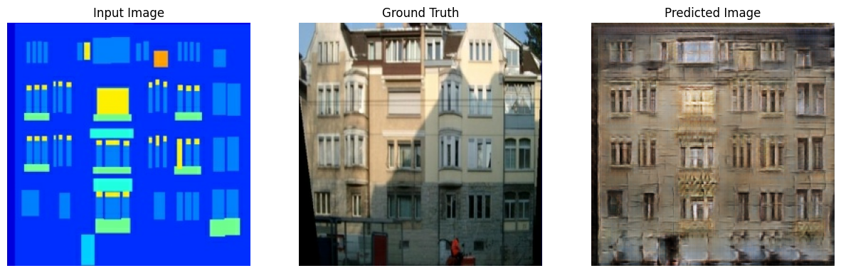
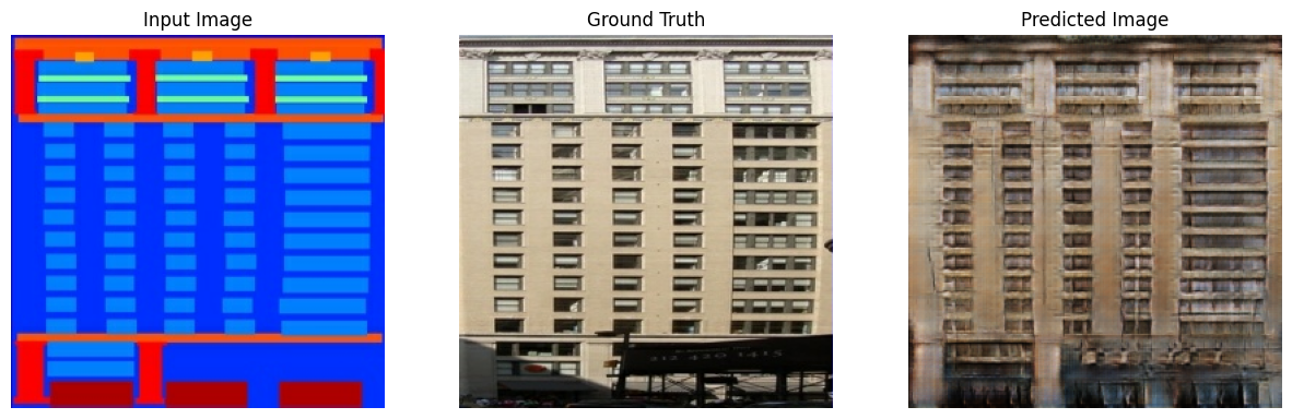
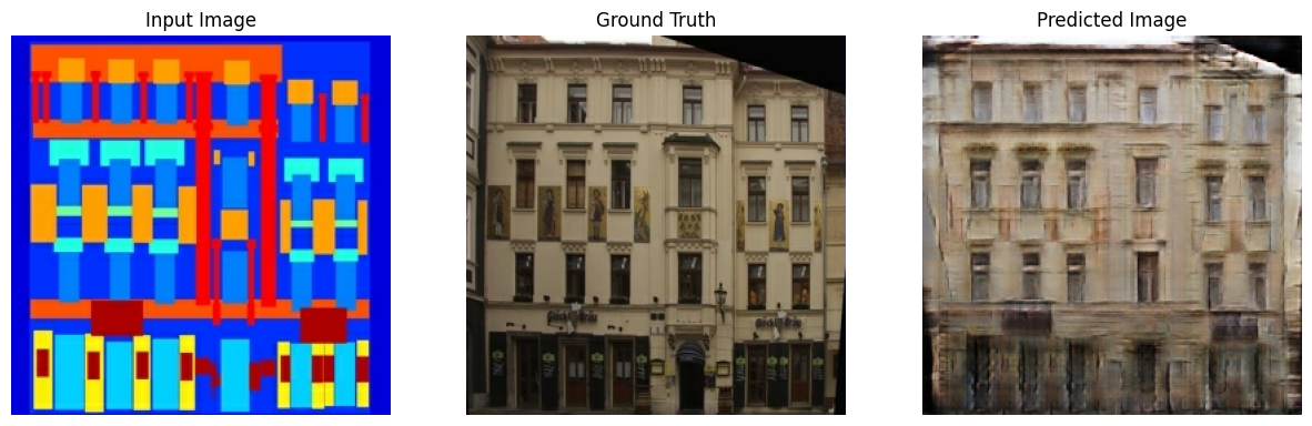
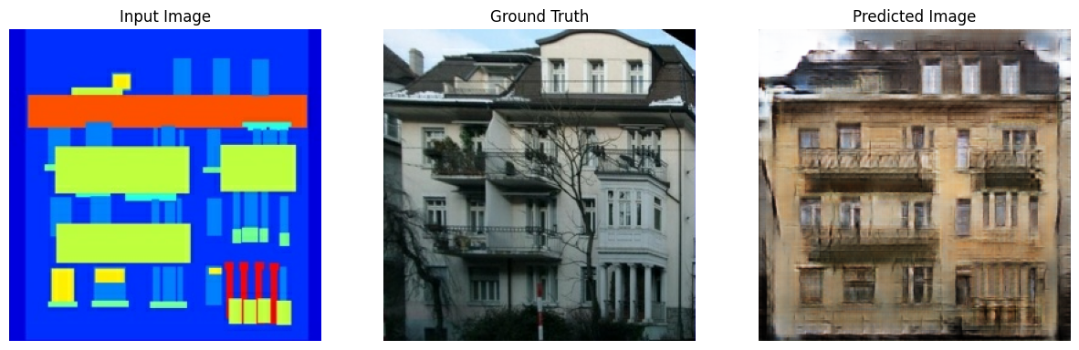
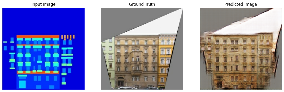
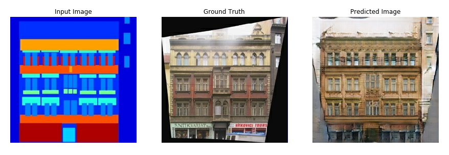
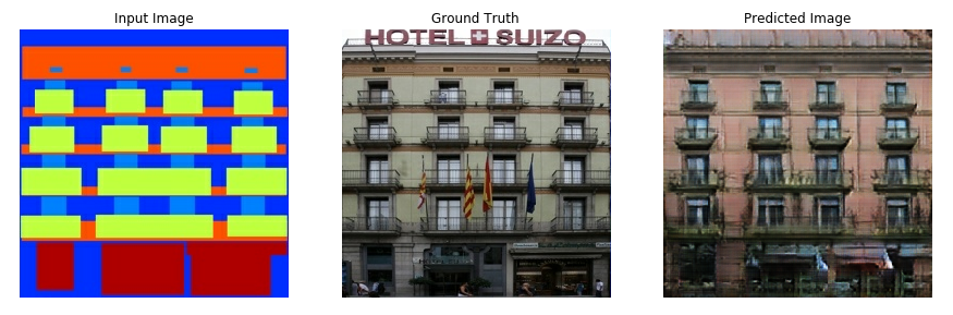
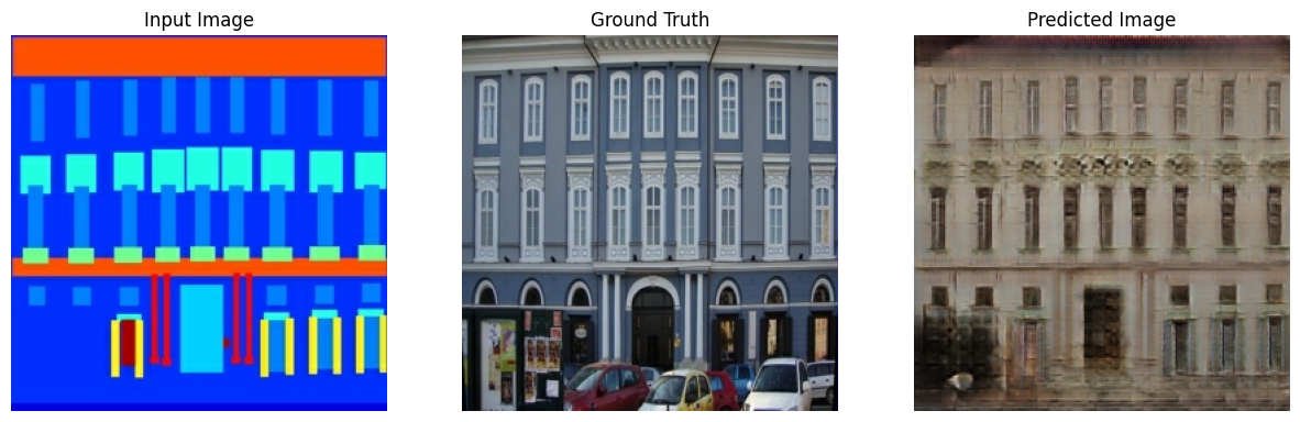
Below are some examples of the output generated by the pix2pix cGAN after training for 200 epochs on the facades dataset (80k steps).
Import TensorFlow and other libraries
import tensorflow as tf

import os
import pathlib
import time
import datetime

from matplotlib import pyplot as plt
from IPython import display
2024-08-16 05:11:33.561479: E external/local_xla/xla/stream_executor/cuda/cuda_fft.cc:485] Unable to register cuFFT factory: Attempting to register factory for plugin cuFFT when one has already been registered
2024-08-16 05:11:33.582597: E external/local_xla/xla/stream_executor/cuda/cuda_dnn.cc:8454] Unable to register cuDNN factory: Attempting to register factory for plugin cuDNN when one has already been registered
2024-08-16 05:11:33.589027: E external/local_xla/xla/stream_executor/cuda/cuda_blas.cc:1452] Unable to register cuBLAS factory: Attempting to register factory for plugin cuBLAS when one has already been registered
Load the dataset
Download the CMP Facade Database data (30MB). Additional datasets are available in the same format here. In Colab you can select other datasets from the drop-down menu. Note that some of the other datasets are significantly larger (edges2handbags is 8GB in size).
dataset_name = "facades"
_URL = f'http://efrosgans.eecs.berkeley.edu/pix2pix/datasets/{dataset_name}.tar.gz'

path_to_zip = tf.keras.utils.get_file(
    fname=f"{dataset_name}.tar.gz",
    origin=_URL,
    extract=True)

path_to_zip  = pathlib.Path(path_to_zip)

PATH = path_to_zip.parent/dataset_name
Downloading data from http://efrosgans.eecs.berkeley.edu/pix2pix/datasets/facades.tar.gz
30168306/30168306 ━━━━━━━━━━━━━━━━━━━━ 8s 0us/step
list(PATH.parent.iterdir())
[PosixPath('/home/kbuilder/.keras/datasets/flower_photos.tar'),
 PosixPath('/home/kbuilder/.keras/datasets/fashion-mnist'),
 PosixPath('/home/kbuilder/.keras/datasets/mnist.npz'),
 PosixPath('/home/kbuilder/.keras/datasets/HIGGS.csv.gz'),
 PosixPath('/home/kbuilder/.keras/datasets/facades.tar.gz'),
 PosixPath('/home/kbuilder/.keras/datasets/jena_climate_2009_2016.csv'),
 PosixPath('/home/kbuilder/.keras/datasets/iris_test.csv'),
 PosixPath('/home/kbuilder/.keras/datasets/cats_and_dogs_filtered'),
 PosixPath('/home/kbuilder/.keras/datasets/jena_climate_2009_2016.csv.zip'),
 PosixPath('/home/kbuilder/.keras/datasets/facades'),
 PosixPath('/home/kbuilder/.keras/datasets/cifar-10-batches-py'),
 PosixPath('/home/kbuilder/.keras/datasets/kandinsky5.jpg'),
 PosixPath('/home/kbuilder/.keras/datasets/iris_training.csv'),
 PosixPath('/home/kbuilder/.keras/datasets/cats_and_dogs.zip'),
 PosixPath('/home/kbuilder/.keras/datasets/Red_sunflower'),
 PosixPath('/home/kbuilder/.keras/datasets/cifar-10-batches-py.tar.gz'),
 PosixPath('/home/kbuilder/.keras/datasets/YellowLabradorLooking_new.jpg'),
 PosixPath('/home/kbuilder/.keras/datasets/flower_photos')]
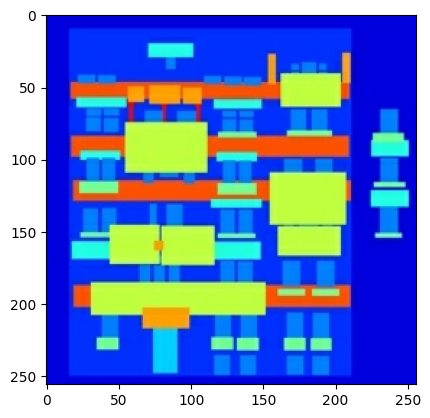
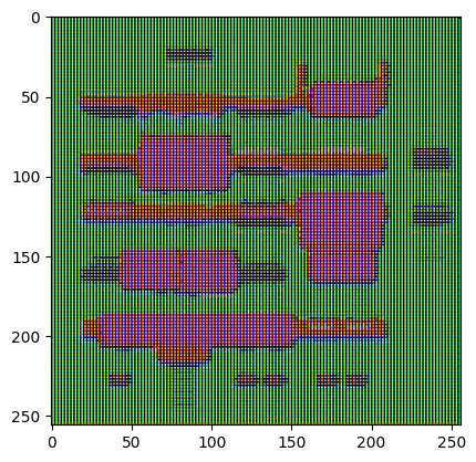
Each original image is of size 256 x 512 containing two 256 x 256 images:
sample_image = tf.io.read_file(str(PATH / 'train/1.jpg'))
sample_image = tf.io.decode_jpeg(sample_image)
print(sample_image.shape)
(256, 512, 3)
WARNING: All log messages before absl::InitializeLog() is called are written to STDERR
I0000 00:00:1723785104.657821  166285 cuda_executor.cc:1015] successful NUMA node read from SysFS had negative value (-1), but there must be at least one NUMA node, so returning NUMA node zero. See more at https://github.com/torvalds/linux/blob/v6.0/Documentation/ABI/testing/sysfs-bus-pci#L344-L355
I0000 00:00:1723785104.661724  166285 cuda_executor.cc:1015] successful NUMA node read from SysFS had negative value (-1), but there must be at least one NUMA node, so returning NUMA node zero. See more at https://github.com/torvalds/linux/blob/v6.0/Documentation/ABI/testing/sysfs-bus-pci#L344-L355
I0000 00:00:1723785104.665422  166285 cuda_executor.cc:1015] successful NUMA node read from SysFS had negative value (-1), but there must be at least one NUMA node, so returning NUMA node zero. See more at https://github.com/torvalds/linux/blob/v6.0/Documentation/ABI/testing/sysfs-bus-pci#L344-L355
I0000 00:00:1723785104.669063  166285 cuda_executor.cc:1015] successful NUMA node read from SysFS had negative value (-1), but there must be at least one NUMA node, so returning NUMA node zero. See more at https://github.com/torvalds/linux/blob/v6.0/Documentation/ABI/testing/sysfs-bus-pci#L344-L355
I0000 00:00:1723785104.681592  166285 cuda_executor.cc:1015] successful NUMA node read from SysFS had negative value (-1), but there must be at least one NUMA node, so returning NUMA node zero. See more at https://github.com/torvalds/linux/blob/v6.0/Documentation/ABI/testing/sysfs-bus-pci#L344-L355
I0000 00:00:1723785104.685097  166285 cuda_executor.cc:1015] successful NUMA node read from SysFS had negative value (-1), but there must be at least one NUMA node, so returning NUMA node zero. See more at https://github.com/torvalds/linux/blob/v6.0/Documentation/ABI/testing/sysfs-bus-pci#L344-L355
I0000 00:00:1723785104.688447  166285 cuda_executor.cc:1015] successful NUMA node read from SysFS had negative value (-1), but there must be at least one NUMA node, so returning NUMA node zero. See more at https://github.com/torvalds/linux/blob/v6.0/Documentation/ABI/testing/sysfs-bus-pci#L344-L355
I0000 00:00:1723785104.691826  166285 cuda_executor.cc:1015] successful NUMA node read from SysFS had negative value (-1), but there must be at least one NUMA node, so returning NUMA node zero. See more at https://github.com/torvalds/linux/blob/v6.0/Documentation/ABI/testing/sysfs-bus-pci#L344-L355
I0000 00:00:1723785104.695256  166285 cuda_executor.cc:1015] successful NUMA node read from SysFS had negative value (-1), but there must be at least one NUMA node, so returning NUMA node zero. See more at https://github.com/torvalds/linux/blob/v6.0/Documentation/ABI/testing/sysfs-bus-pci#L344-L355
I0000 00:00:1723785104.698866  166285 cuda_executor.cc:1015] successful NUMA node read from SysFS had negative value (-1), but there must be at least one NUMA node, so returning NUMA node zero. See more at https://github.com/torvalds/linux/blob/v6.0/Documentation/ABI/testing/sysfs-bus-pci#L344-L355
I0000 00:00:1723785104.702269  166285 cuda_executor.cc:1015] successful NUMA node read from SysFS had negative value (-1), but there must be at least one NUMA node, so returning NUMA node zero. See more at https://github.com/torvalds/linux/blob/v6.0/Documentation/ABI/testing/sysfs-bus-pci#L344-L355
I0000 00:00:1723785104.705685  166285 cuda_executor.cc:1015] successful NUMA node read from SysFS had negative value (-1), but there must be at least one NUMA node, so returning NUMA node zero. See more at https://github.com/torvalds/linux/blob/v6.0/Documentation/ABI/testing/sysfs-bus-pci#L344-L355
I0000 00:00:1723785105.940631  166285 cuda_executor.cc:1015] successful NUMA node read from SysFS had negative value (-1), but there must be at least one NUMA node, so returning NUMA node zero. See more at https://github.com/torvalds/linux/blob/v6.0/Documentation/ABI/testing/sysfs-bus-pci#L344-L355
I0000 00:00:1723785105.942787  166285 cuda_executor.cc:1015] successful NUMA node read from SysFS had negative value (-1), but there must be at least one NUMA node, so returning NUMA node zero. See more at https://github.com/torvalds/linux/blob/v6.0/Documentation/ABI/testing/sysfs-bus-pci#L344-L355
I0000 00:00:1723785105.944821  166285 cuda_executor.cc:1015] successful NUMA node read from SysFS had negative value (-1), but there must be at least one NUMA node, so returning NUMA node zero. See more at https://github.com/torvalds/linux/blob/v6.0/Documentation/ABI/testing/sysfs-bus-pci#L344-L355
I0000 00:00:1723785105.946901  166285 cuda_executor.cc:1015] successful NUMA node read from SysFS had negative value (-1), but there must be at least one NUMA node, so returning NUMA node zero. See more at https://github.com/torvalds/linux/blob/v6.0/Documentation/ABI/testing/sysfs-bus-pci#L344-L355
I0000 00:00:1723785105.948931  166285 cuda_executor.cc:1015] successful NUMA node read from SysFS had negative value (-1), but there must be at least one NUMA node, so returning NUMA node zero. See more at https://github.com/torvalds/linux/blob/v6.0/Documentation/ABI/testing/sysfs-bus-pci#L344-L355
I0000 00:00:1723785105.950912  166285 cuda_executor.cc:1015] successful NUMA node read from SysFS had negative value (-1), but there must be at least one NUMA node, so returning NUMA node zero. See more at https://github.com/torvalds/linux/blob/v6.0/Documentation/ABI/testing/sysfs-bus-pci#L344-L355
I0000 00:00:1723785105.952829  166285 cuda_executor.cc:1015] successful NUMA node read from SysFS had negative value (-1), but there must be at least one NUMA node, so returning NUMA node zero. See more at https://github.com/torvalds/linux/blob/v6.0/Documentation/ABI/testing/sysfs-bus-pci#L344-L355
I0000 00:00:1723785105.954858  166285 cuda_executor.cc:1015] successful NUMA node read from SysFS had negative value (-1), but there must be at least one NUMA node, so returning NUMA node zero. See more at https://github.com/torvalds/linux/blob/v6.0/Documentation/ABI/testing/sysfs-bus-pci#L344-L355
I0000 00:00:1723785105.956710  166285 cuda_executor.cc:1015] successful NUMA node read from SysFS had negative value (-1), but there must be at least one NUMA node, so returning NUMA node zero. See more at https://github.com/torvalds/linux/blob/v6.0/Documentation/ABI/testing/sysfs-bus-pci#L344-L355
I0000 00:00:1723785105.958713  166285 cuda_executor.cc:1015] successful NUMA node read from SysFS had negative value (-1), but there must be at least one NUMA node, so returning NUMA node zero. See more at https://github.com/torvalds/linux/blob/v6.0/Documentation/ABI/testing/sysfs-bus-pci#L344-L355
I0000 00:00:1723785105.960654  166285 cuda_executor.cc:1015] successful NUMA node read from SysFS had negative value (-1), but there must be at least one NUMA node, so returning NUMA node zero. See more at https://github.com/torvalds/linux/blob/v6.0/Documentation/ABI/testing/sysfs-bus-pci#L344-L355
I0000 00:00:1723785105.962741  166285 cuda_executor.cc:1015] successful NUMA node read from SysFS had negative value (-1), but there must be at least one NUMA node, so returning NUMA node zero. See more at https://github.com/torvalds/linux/blob/v6.0/Documentation/ABI/testing/sysfs-bus-pci#L344-L355
I0000 00:00:1723785106.001208  166285 cuda_executor.cc:1015] successful NUMA node read from SysFS had negative value (-1), but there must be at least one NUMA node, so returning NUMA node zero. See more at https://github.com/torvalds/linux/blob/v6.0/Documentation/ABI/testing/sysfs-bus-pci#L344-L355
I0000 00:00:1723785106.003283  166285 cuda_executor.cc:1015] successful NUMA node read from SysFS had negative value (-1), but there must be at least one NUMA node, so returning NUMA node zero. See more at https://github.com/torvalds/linux/blob/v6.0/Documentation/ABI/testing/sysfs-bus-pci#L344-L355
I0000 00:00:1723785106.005256  166285 cuda_executor.cc:1015] successful NUMA node read from SysFS had negative value (-1), but there must be at least one NUMA node, so returning NUMA node zero. See more at https://github.com/torvalds/linux/blob/v6.0/Documentation/ABI/testing/sysfs-bus-pci#L344-L355
I0000 00:00:1723785106.007288  166285 cuda_executor.cc:1015] successful NUMA node read from SysFS had negative value (-1), but there must be at least one NUMA node, so returning NUMA node zero. See more at https://github.com/torvalds/linux/blob/v6.0/Documentation/ABI/testing/sysfs-bus-pci#L344-L355
I0000 00:00:1723785106.009146  166285 cuda_executor.cc:1015] successful NUMA node read from SysFS had negative value (-1), but there must be at least one NUMA node, so returning NUMA node zero. See more at https://github.com/torvalds/linux/blob/v6.0/Documentation/ABI/testing/sysfs-bus-pci#L344-L355
I0000 00:00:1723785106.011252  166285 cuda_executor.cc:1015] successful NUMA node read from SysFS had negative value (-1), but there must be at least one NUMA node, so returning NUMA node zero. See more at https://github.com/torvalds/linux/blob/v6.0/Documentation/ABI/testing/sysfs-bus-pci#L344-L355
I0000 00:00:1723785106.013222  166285 cuda_executor.cc:1015] successful NUMA node read from SysFS had negative value (-1), but there must be at least one NUMA node, so returning NUMA node zero. See more at https://github.com/torvalds/linux/blob/v6.0/Documentation/ABI/testing/sysfs-bus-pci#L344-L355
I0000 00:00:1723785106.015226  166285 cuda_executor.cc:1015] successful NUMA node read from SysFS had negative value (-1), but there must be at least one NUMA node, so returning NUMA node zero. See more at https://github.com/torvalds/linux/blob/v6.0/Documentation/ABI/testing/sysfs-bus-pci#L344-L355
I0000 00:00:1723785106.017081  166285 cuda_executor.cc:1015] successful NUMA node read from SysFS had negative value (-1), but there must be at least one NUMA node, so returning NUMA node zero. See more at https://github.com/torvalds/linux/blob/v6.0/Documentation/ABI/testing/sysfs-bus-pci#L344-L355
I0000 00:00:1723785106.019604  166285 cuda_executor.cc:1015] successful NUMA node read from SysFS had negative value (-1), but there must be at least one NUMA node, so returning NUMA node zero. See more at https://github.com/torvalds/linux/blob/v6.0/Documentation/ABI/testing/sysfs-bus-pci#L344-L355
I0000 00:00:1723785106.021954  166285 cuda_executor.cc:1015] successful NUMA node read from SysFS had negative value (-1), but there must be at least one NUMA node, so returning NUMA node zero. See more at https://github.com/torvalds/linux/blob/v6.0/Documentation/ABI/testing/sysfs-bus-pci#L344-L355
I0000 00:00:1723785106.024390  166285 cuda_executor.cc:1015] successful NUMA node read from SysFS had negative value (-1), but there must be at least one NUMA node, so returning NUMA node zero. See more at https://github.com/torvalds/linux/blob/v6.0/Documentation/ABI/testing/sysfs-bus-pci#L344-L355
plt.figure()
plt.imshow(sample_image)
<matplotlib.image.AxesImage at 0x7f1607efcfd0>
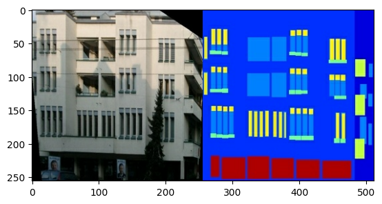
You need to separate real building facade images from the architecture label images—all of which will be of size 256 x 256.
Define a function that loads image files and outputs two image tensors:
def load(image_file):
  # Read and decode an image file to a uint8 tensor
  image = tf.io.read_file(image_file)
  image = tf.io.decode_jpeg(image)

  # Split each image tensor into two tensors:
  # - one with a real building facade image
  # - one with an architecture label image
  w = tf.shape(image)[1]
  w = w // 2
  input_image = image[:, w:, :]
  real_image = image[:, :w, :]

  # Convert both images to float32 tensors
  input_image = tf.cast(input_image, tf.float32)
  real_image = tf.cast(real_image, tf.float32)

  return input_image, real_image
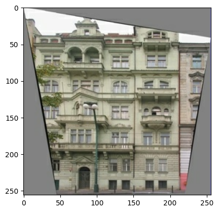
Plot a sample of the input (architecture label image) and real (building facade photo) images:
inp, re = load(str(PATH / 'train/100.jpg'))
# Casting to int for matplotlib to display the images
plt.figure()
plt.imshow(inp / 255.0)
plt.figure()
plt.imshow(re / 255.0)
<matplotlib.image.AxesImage at 0x7f15f031bdf0>
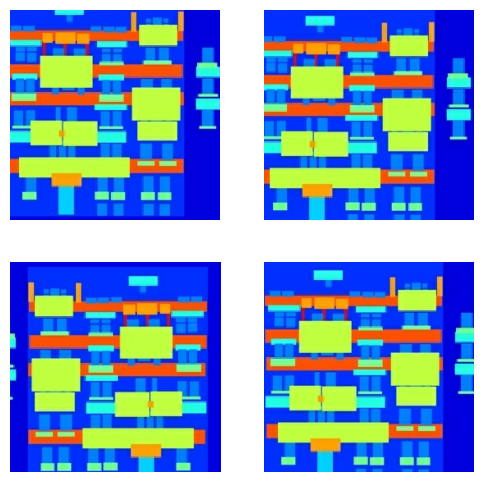
As described in the pix2pix paper, you need to apply random jittering and mirroring to preprocess the training set.
Define several functions that:
- Resize each
256 x 256image to a larger height and width—286 x 286. - Randomly crop it back to
256 x 256. - Randomly flip the image horizontally i.e., left to right (random mirroring).
- Normalize the images to the
[-1, 1]range.
# The facade training set consist of 400 images
BUFFER_SIZE = 400
# The batch size of 1 produced better results for the U-Net in the original pix2pix experiment
BATCH_SIZE = 1
# Each image is 256x256 in size
IMG_WIDTH = 256
IMG_HEIGHT = 256
def resize(input_image, real_image, height, width):
  input_image = tf.image.resize(input_image, [height, width],
                                method=tf.image.ResizeMethod.NEAREST_NEIGHBOR)
  real_image = tf.image.resize(real_image, [height, width],
                               method=tf.image.ResizeMethod.NEAREST_NEIGHBOR)

  return input_image, real_image
def random_crop(input_image, real_image):
  stacked_image = tf.stack([input_image, real_image], axis=0)
  cropped_image = tf.image.random_crop(
      stacked_image, size=[2, IMG_HEIGHT, IMG_WIDTH, 3])

  return cropped_image[0], cropped_image[1]
# Normalizing the images to [-1, 1]
def normalize(input_image, real_image):
  input_image = (input_image / 127.5) - 1
  real_image = (real_image / 127.5) - 1

  return input_image, real_image
@tf.function()
def random_jitter(input_image, real_image):
  # Resizing to 286x286
  input_image, real_image = resize(input_image, real_image, 286, 286)

  # Random cropping back to 256x256
  input_image, real_image = random_crop(input_image, real_image)

  if tf.random.uniform(()) > 0.5:
    # Random mirroring
    input_image = tf.image.flip_left_right(input_image)
    real_image = tf.image.flip_left_right(real_image)

  return input_image, real_image
You can inspect some of the preprocessed output:
plt.figure(figsize=(6, 6))
for i in range(4):
  rj_inp, rj_re = random_jitter(inp, re)
  plt.subplot(2, 2, i + 1)
  plt.imshow(rj_inp / 255.0)
  plt.axis('off')
plt.show()
Having checked that the loading and preprocessing works, let's define a couple of helper functions that load and preprocess the training and test sets:
def load_image_train(image_file):
  input_image, real_image = load(image_file)
  input_image, real_image = random_jitter(input_image, real_image)
  input_image, real_image = normalize(input_image, real_image)

  return input_image, real_image
def load_image_test(image_file):
  input_image, real_image = load(image_file)
  input_image, real_image = resize(input_image, real_image,
                                   IMG_HEIGHT, IMG_WIDTH)
  input_image, real_image = normalize(input_image, real_image)

  return input_image, real_image
Build an input pipeline with tf.data
train_dataset = tf.data.Dataset.list_files(str(PATH / 'train/*.jpg'))
train_dataset = train_dataset.map(load_image_train,
                                  num_parallel_calls=tf.data.AUTOTUNE)
train_dataset = train_dataset.shuffle(BUFFER_SIZE)
train_dataset = train_dataset.batch(BATCH_SIZE)
try:
  test_dataset = tf.data.Dataset.list_files(str(PATH / 'test/*.jpg'))
except tf.errors.InvalidArgumentError:
  test_dataset = tf.data.Dataset.list_files(str(PATH / 'val/*.jpg'))
test_dataset = test_dataset.map(load_image_test)
test_dataset = test_dataset.batch(BATCH_SIZE)
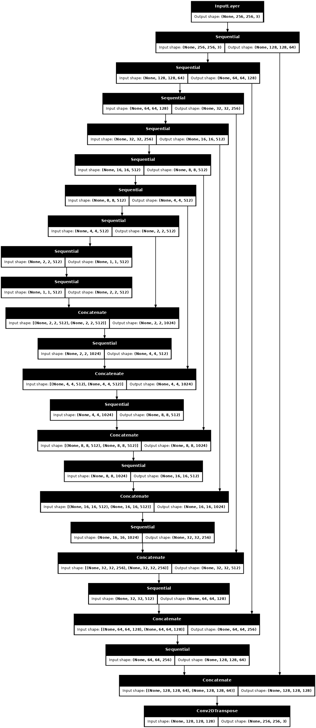
Build the generator
The generator of your pix2pix cGAN is a modified U-Net. A U-Net consists of an encoder (downsampler) and decoder (upsampler). (You can find out more about it in the Image segmentation tutorial and on the U-Net project website.)
- Each block in the encoder is: Convolution -> Batch normalization -> Leaky ReLU
- Each block in the decoder is: Transposed convolution -> Batch normalization -> Dropout (applied to the first 3 blocks) -> ReLU
- There are skip connections between the encoder and decoder (as in the U-Net).
Define the downsampler (encoder):
OUTPUT_CHANNELS = 3
def downsample(filters, size, apply_batchnorm=True):
  initializer = tf.random_normal_initializer(0., 0.02)

  result = tf.keras.Sequential()
  result.add(
      tf.keras.layers.Conv2D(filters, size, strides=2, padding='same',
                             kernel_initializer=initializer, use_bias=False))

  if apply_batchnorm:
    result.add(tf.keras.layers.BatchNormalization())

  result.add(tf.keras.layers.LeakyReLU())

  return result
down_model = downsample(3, 4)
down_result = down_model(tf.expand_dims(inp, 0))
print (down_result.shape)
(1, 128, 128, 3)
W0000 00:00:1723785108.147399  166285 gpu_timer.cc:114] Skipping the delay kernel, measurement accuracy will be reduced
W0000 00:00:1723785108.182976  166285 gpu_timer.cc:114] Skipping the delay kernel, measurement accuracy will be reduced
W0000 00:00:1723785108.221808  166285 gpu_timer.cc:114] Skipping the delay kernel, measurement accuracy will be reduced
W0000 00:00:1723785108.230772  166285 gpu_timer.cc:114] Skipping the delay kernel, measurement accuracy will be reduced
W0000 00:00:1723785108.231959  166285 gpu_timer.cc:114] Skipping the delay kernel, measurement accuracy will be reduced
W0000 00:00:1723785108.235100  166285 gpu_timer.cc:114] Skipping the delay kernel, measurement accuracy will be reduced
W0000 00:00:1723785108.238282  166285 gpu_timer.cc:114] Skipping the delay kernel, measurement accuracy will be reduced
W0000 00:00:1723785108.239508  166285 gpu_timer.cc:114] Skipping the delay kernel, measurement accuracy will be reduced
W0000 00:00:1723785108.240794  166285 gpu_timer.cc:114] Skipping the delay kernel, measurement accuracy will be reduced
W0000 00:00:1723785108.242041  166285 gpu_timer.cc:114] Skipping the delay kernel, measurement accuracy will be reduced
W0000 00:00:1723785108.243196  166285 gpu_timer.cc:114] Skipping the delay kernel, measurement accuracy will be reduced
W0000 00:00:1723785108.244345  166285 gpu_timer.cc:114] Skipping the delay kernel, measurement accuracy will be reduced
W0000 00:00:1723785108.245526  166285 gpu_timer.cc:114] Skipping the delay kernel, measurement accuracy will be reduced
W0000 00:00:1723785108.246742  166285 gpu_timer.cc:114] Skipping the delay kernel, measurement accuracy will be reduced
Define the upsampler (decoder):
def upsample(filters, size, apply_dropout=False):
  initializer = tf.random_normal_initializer(0., 0.02)

  result = tf.keras.Sequential()
  result.add(
    tf.keras.layers.Conv2DTranspose(filters, size, strides=2,
                                    padding='same',
                                    kernel_initializer=initializer,
                                    use_bias=False))

  result.add(tf.keras.layers.BatchNormalization())

  if apply_dropout:
      result.add(tf.keras.layers.Dropout(0.5))

  result.add(tf.keras.layers.ReLU())

  return result
up_model = upsample(3, 4)
up_result = up_model(down_result)
print (up_result.shape)
(1, 256, 256, 3)
W0000 00:00:1723785108.377660  166285 gpu_timer.cc:114] Skipping the delay kernel, measurement accuracy will be reduced
W0000 00:00:1723785108.387068  166285 gpu_timer.cc:114] Skipping the delay kernel, measurement accuracy will be reduced
W0000 00:00:1723785108.388344  166285 gpu_timer.cc:114] Skipping the delay kernel, measurement accuracy will be reduced
W0000 00:00:1723785108.389669  166285 gpu_timer.cc:114] Skipping the delay kernel, measurement accuracy will be reduced
W0000 00:00:1723785108.455281  166285 gpu_timer.cc:114] Skipping the delay kernel, measurement accuracy will be reduced
W0000 00:00:1723785108.457890  166285 gpu_timer.cc:114] Skipping the delay kernel, measurement accuracy will be reduced
W0000 00:00:1723785108.484726  166285 gpu_timer.cc:114] Skipping the delay kernel, measurement accuracy will be reduced
W0000 00:00:1723785108.495839  166285 gpu_timer.cc:114] Skipping the delay kernel, measurement accuracy will be reduced
Define the generator with the downsampler and the upsampler:
def Generator():
  inputs = tf.keras.layers.Input(shape=[256, 256, 3])

  down_stack = [
    downsample(64, 4, apply_batchnorm=False),  # (batch_size, 128, 128, 64)
    downsample(128, 4),  # (batch_size, 64, 64, 128)
    downsample(256, 4),  # (batch_size, 32, 32, 256)
    downsample(512, 4),  # (batch_size, 16, 16, 512)
    downsample(512, 4),  # (batch_size, 8, 8, 512)
    downsample(512, 4),  # (batch_size, 4, 4, 512)
    downsample(512, 4),  # (batch_size, 2, 2, 512)
    downsample(512, 4),  # (batch_size, 1, 1, 512)
  ]

  up_stack = [
    upsample(512, 4, apply_dropout=True),  # (batch_size, 2, 2, 1024)
    upsample(512, 4, apply_dropout=True),  # (batch_size, 4, 4, 1024)
    upsample(512, 4, apply_dropout=True),  # (batch_size, 8, 8, 1024)
    upsample(512, 4),  # (batch_size, 16, 16, 1024)
    upsample(256, 4),  # (batch_size, 32, 32, 512)
    upsample(128, 4),  # (batch_size, 64, 64, 256)
    upsample(64, 4),  # (batch_size, 128, 128, 128)
  ]

  initializer = tf.random_normal_initializer(0., 0.02)
  last = tf.keras.layers.Conv2DTranspose(OUTPUT_CHANNELS, 4,
                                         strides=2,
                                         padding='same',
                                         kernel_initializer=initializer,
                                         activation='tanh')  # (batch_size, 256, 256, 3)

  x = inputs

  # Downsampling through the model
  skips = []
  for down in down_stack:
    x = down(x)
    skips.append(x)

  skips = reversed(skips[:-1])

  # Upsampling and establishing the skip connections
  for up, skip in zip(up_stack, skips):
    x = up(x)
    x = tf.keras.layers.Concatenate()([x, skip])

  x = last(x)

  return tf.keras.Model(inputs=inputs, outputs=x)
Visualize the generator model architecture:
generator = Generator()
tf.keras.utils.plot_model(generator, show_shapes=True, dpi=64)
Test the generator:
gen_output = generator(inp[tf.newaxis, ...], training=False)
plt.imshow(gen_output[0, ...])
W0000 00:00:1723785109.096026  166285 gpu_timer.cc:114] Skipping the delay kernel, measurement accuracy will be reduced
W0000 00:00:1723785109.097619  166285 gpu_timer.cc:114] Skipping the delay kernel, measurement accuracy will be reduced
W0000 00:00:1723785109.098841  166285 gpu_timer.cc:114] Skipping the delay kernel, measurement accuracy will be reduced
W0000 00:00:1723785109.100040  166285 gpu_timer.cc:114] Skipping the delay kernel, measurement accuracy will be reduced
W0000 00:00:1723785109.101229  166285 gpu_timer.cc:114] Skipping the delay kernel, measurement accuracy will be reduced
W0000 00:00:1723785109.102429  166285 gpu_timer.cc:114] Skipping the delay kernel, measurement accuracy will be reduced
W0000 00:00:1723785109.103610  166285 gpu_timer.cc:114] Skipping the delay kernel, measurement accuracy will be reduced
W0000 00:00:1723785109.104793  166285 gpu_timer.cc:114] Skipping the delay kernel, measurement accuracy will be reduced
W0000 00:00:1723785109.106177  166285 gpu_timer.cc:114] Skipping the delay kernel, measurement accuracy will be reduced
W0000 00:00:1723785109.107435  166285 gpu_timer.cc:114] Skipping the delay kernel, measurement accuracy will be reduced
W0000 00:00:1723785109.108671  166285 gpu_timer.cc:114] Skipping the delay kernel, measurement accuracy will be reduced
W0000 00:00:1723785109.109909  166285 gpu_timer.cc:114] Skipping the delay kernel, measurement accuracy will be reduced
W0000 00:00:1723785109.111149  166285 gpu_timer.cc:114] Skipping the delay kernel, measurement accuracy will be reduced
W0000 00:00:1723785109.121879  166285 gpu_timer.cc:114] Skipping the delay kernel, measurement accuracy will be reduced
W0000 00:00:1723785109.123521  166285 gpu_timer.cc:114] Skipping the delay kernel, measurement accuracy will be reduced
W0000 00:00:1723785109.125140  166285 gpu_timer.cc:114] Skipping the delay kernel, measurement accuracy will be reduced
W0000 00:00:1723785109.126800  166285 gpu_timer.cc:114] Skipping the delay kernel, measurement accuracy will be reduced
W0000 00:00:1723785109.128454  166285 gpu_timer.cc:114] Skipping the delay kernel, measurement accuracy will be reduced
W0000 00:00:1723785109.130235  166285 gpu_timer.cc:114] Skipping the delay kernel, measurement accuracy will be reduced
W0000 00:00:1723785109.132077  166285 gpu_timer.cc:114] Skipping the delay kernel, measurement accuracy will be reduced
W0000 00:00:1723785109.133884  166285 gpu_timer.cc:114] Skipping the delay kernel, measurement accuracy will be reduced
W0000 00:00:1723785109.135697  166285 gpu_timer.cc:114] Skipping the delay kernel, measurement accuracy will be reduced
W0000 00:00:1723785109.137506  166285 gpu_timer.cc:114] Skipping the delay kernel, measurement accuracy will be reduced
W0000 00:00:1723785109.155481  166285 gpu_timer.cc:114] Skipping the delay kernel, measurement accuracy will be reduced
W0000 00:00:1723785109.157454  166285 gpu_timer.cc:114] Skipping the delay kernel, measurement accuracy will be reduced
W0000 00:00:1723785109.159616  166285 gpu_timer.cc:114] Skipping the delay kernel, measurement accuracy will be reduced
W0000 00:00:1723785109.161774  166285 gpu_timer.cc:114] Skipping the delay kernel, measurement accuracy will be reduced
W0000 00:00:1723785109.176307  166285 gpu_timer.cc:114] Skipping the delay kernel, measurement accuracy will be reduced
W0000 00:00:1723785109.178050  166285 gpu_timer.cc:114] Skipping the delay kernel, measurement accuracy will be reduced
W0000 00:00:1723785109.179745  166285 gpu_timer.cc:114] Skipping the delay kernel, measurement accuracy will be reduced
W0000 00:00:1723785109.181487  166285 gpu_timer.cc:114] Skipping the delay kernel, measurement accuracy will be reduced
W0000 00:00:1723785109.183223  166285 gpu_timer.cc:114] Skipping the delay kernel, measurement accuracy will be reduced
W0000 00:00:1723785109.185037  166285 gpu_timer.cc:114] Skipping the delay kernel, measurement accuracy will be reduced
W0000 00:00:1723785109.186854  166285 gpu_timer.cc:114] Skipping the delay kernel, measurement accuracy will be reduced
W0000 00:00:1723785109.188678  166285 gpu_timer.cc:114] Skipping the delay kernel, measurement accuracy will be reduced
W0000 00:00:1723785109.190863  166285 gpu_timer.cc:114] Skipping the delay kernel, measurement accuracy will be reduced
W0000 00:00:1723785109.192884  166285 gpu_timer.cc:114] Skipping the delay kernel, measurement accuracy will be reduced
W0000 00:00:1723785109.195094  166285 gpu_timer.cc:114] Skipping the delay kernel, measurement accuracy will be reduced
W0000 00:00:1723785109.197117  166285 gpu_timer.cc:114] Skipping the delay kernel, measurement accuracy will be reduced
W0000 00:00:1723785109.199278  166285 gpu_timer.cc:114] Skipping the delay kernel, measurement accuracy will be reduced
W0000 00:00:1723785109.201419  166285 gpu_timer.cc:114] Skipping the delay kernel, measurement accuracy will be reduced
W0000 00:00:1723785109.215509  166285 gpu_timer.cc:114] Skipping the delay kernel, measurement accuracy will be reduced
W0000 00:00:1723785109.217281  166285 gpu_timer.cc:114] Skipping the delay kernel, measurement accuracy will be reduced
W0000 00:00:1723785109.223448  166285 gpu_timer.cc:114] Skipping the delay kernel, measurement accuracy will be reduced
W0000 00:00:1723785109.225682  166285 gpu_timer.cc:114] Skipping the delay kernel, measurement accuracy will be reduced
W0000 00:00:1723785109.227776  166285 gpu_timer.cc:114] Skipping the delay kernel, measurement accuracy will be reduced
W0000 00:00:1723785109.230031  166285 gpu_timer.cc:114] Skipping the delay kernel, measurement accuracy will be reduced
W0000 00:00:1723785109.232352  166285 gpu_timer.cc:114] Skipping the delay kernel, measurement accuracy will be reduced
W0000 00:00:1723785109.234662  166285 gpu_timer.cc:114] Skipping the delay kernel, measurement accuracy will be reduced
W0000 00:00:1723785109.236991  166285 gpu_timer.cc:114] Skipping the delay kernel, measurement accuracy will be reduced
W0000 00:00:1723785109.239215  166285 gpu_timer.cc:114] Skipping the delay kernel, measurement accuracy will be reduced
W0000 00:00:1723785109.241617  166285 gpu_timer.cc:114] Skipping the delay kernel, measurement accuracy will be reduced
W0000 00:00:1723785109.243976  166285 gpu_timer.cc:114] Skipping the delay kernel, measurement accuracy will be reduced
W0000 00:00:1723785109.246326  166285 gpu_timer.cc:114] Skipping the delay kernel, measurement accuracy will be reduced
W0000 00:00:1723785109.249084  166285 gpu_timer.cc:114] Skipping the delay kernel, measurement accuracy will be reduced
W0000 00:00:1723785109.252001  166285 gpu_timer.cc:114] Skipping the delay kernel, measurement accuracy will be reduced
W0000 00:00:1723785109.267926  166285 gpu_timer.cc:114] Skipping the delay kernel, measurement accuracy will be reduced
W0000 00:00:1723785109.270049  166285 gpu_timer.cc:114] Skipping the delay kernel, measurement accuracy will be reduced
W0000 00:00:1723785109.272251  166285 gpu_timer.cc:114] Skipping the delay kernel, measurement accuracy will be reduced
W0000 00:00:1723785109.274554  166285 gpu_timer.cc:114] Skipping the delay kernel, measurement accuracy will be reduced
W0000 00:00:1723785109.285810  166285 gpu_timer.cc:114] Skipping the delay kernel, measurement accuracy will be reduced
W0000 00:00:1723785109.288861  166285 gpu_timer.cc:114] Skipping the delay kernel, measurement accuracy will be reduced
W0000 00:00:1723785109.292116  166285 gpu_timer.cc:114] Skipping the delay kernel, measurement accuracy will be reduced
W0000 00:00:1723785109.295644  166285 gpu_timer.cc:114] Skipping the delay kernel, measurement accuracy will be reduced
W0000 00:00:1723785109.299291  166285 gpu_timer.cc:114] Skipping the delay kernel, measurement accuracy will be reduced
W0000 00:00:1723785109.302788  166285 gpu_timer.cc:114] Skipping the delay kernel, measurement accuracy will be reduced
W0000 00:00:1723785109.306371  166285 gpu_timer.cc:114] Skipping the delay kernel, measurement accuracy will be reduced
W0000 00:00:1723785109.309949  166285 gpu_timer.cc:114] Skipping the delay kernel, measurement accuracy will be reduced
W0000 00:00:1723785109.313319  166285 gpu_timer.cc:114] Skipping the delay kernel, measurement accuracy will be reduced
W0000 00:00:1723785109.316133  166285 gpu_timer.cc:114] Skipping the delay kernel, measurement accuracy will be reduced
W0000 00:00:1723785109.319008  166285 gpu_timer.cc:114] Skipping the delay kernel, measurement accuracy will be reduced
W0000 00:00:1723785109.330585  166285 gpu_timer.cc:114] Skipping the delay kernel, measurement accuracy will be reduced
W0000 00:00:1723785109.332098  166285 gpu_timer.cc:114] Skipping the delay kernel, measurement accuracy will be reduced
W0000 00:00:1723785109.333605  166285 gpu_timer.cc:114] Skipping the delay kernel, measurement accuracy will be reduced
W0000 00:00:1723785109.335154  166285 gpu_timer.cc:114] Skipping the delay kernel, measurement accuracy will be reduced
W0000 00:00:1723785109.337145  166285 gpu_timer.cc:114] Skipping the delay kernel, measurement accuracy will be reduced
W0000 00:00:1723785109.339282  166285 gpu_timer.cc:114] Skipping the delay kernel, measurement accuracy will be reduced
W0000 00:00:1723785109.343361  166285 gpu_timer.cc:114] Skipping the delay kernel, measurement accuracy will be reduced
W0000 00:00:1723785109.345634  166285 gpu_timer.cc:114] Skipping the delay kernel, measurement accuracy will be reduced
W0000 00:00:1723785109.347897  166285 gpu_timer.cc:114] Skipping the delay kernel, measurement accuracy will be reduced
W0000 00:00:1723785109.350160  166285 gpu_timer.cc:114] Skipping the delay kernel, measurement accuracy will be reduced
W0000 00:00:1723785109.352428  166285 gpu_timer.cc:114] Skipping the delay kernel, measurement accuracy will be reduced
W0000 00:00:1723785109.354781  166285 gpu_timer.cc:114] Skipping the delay kernel, measurement accuracy will be reduced
W0000 00:00:1723785109.357124  166285 gpu_timer.cc:114] Skipping the delay kernel, measurement accuracy will be reduced
W0000 00:00:1723785109.359918  166285 gpu_timer.cc:114] Skipping the delay kernel, measurement accuracy will be reduced
W0000 00:00:1723785109.362789  166285 gpu_timer.cc:114] Skipping the delay kernel, measurement accuracy will be reduced
W0000 00:00:1723785109.372654  166285 gpu_timer.cc:114] Skipping the delay kernel, measurement accuracy will be reduced
W0000 00:00:1723785109.374152  166285 gpu_timer.cc:114] Skipping the delay kernel, measurement accuracy will be reduced
W0000 00:00:1723785109.375664  166285 gpu_timer.cc:114] Skipping the delay kernel, measurement accuracy will be reduced
W0000 00:00:1723785109.377213  166285 gpu_timer.cc:114] Skipping the delay kernel, measurement accuracy will be reduced
W0000 00:00:1723785109.379137  166285 gpu_timer.cc:114] Skipping the delay kernel, measurement accuracy will be reduced
W0000 00:00:1723785109.381178  166285 gpu_timer.cc:114] Skipping the delay kernel, measurement accuracy will be reduced
W0000 00:00:1723785109.382680  166285 gpu_timer.cc:114] Skipping the delay kernel, measurement accuracy will be reduced
W0000 00:00:1723785109.384772  166285 gpu_timer.cc:114] Skipping the delay kernel, measurement accuracy will be reduced
W0000 00:00:1723785109.386871  166285 gpu_timer.cc:114] Skipping the delay kernel, measurement accuracy will be reduced
W0000 00:00:1723785109.389035  166285 gpu_timer.cc:114] Skipping the delay kernel, measurement accuracy will be reduced
W0000 00:00:1723785109.391191  166285 gpu_timer.cc:114] Skipping the delay kernel, measurement accuracy will be reduced
W0000 00:00:1723785109.393491  166285 gpu_timer.cc:114] Skipping the delay kernel, measurement accuracy will be reduced
W0000 00:00:1723785109.395801  166285 gpu_timer.cc:114] Skipping the delay kernel, measurement accuracy will be reduced
W0000 00:00:1723785109.398609  166285 gpu_timer.cc:114] Skipping the delay kernel, measurement accuracy will be reduced
W0000 00:00:1723785109.406359  166285 gpu_timer.cc:114] Skipping the delay kernel, measurement accuracy will be reduced
W0000 00:00:1723785109.407827  166285 gpu_timer.cc:114] Skipping the delay kernel, measurement accuracy will be reduced
W0000 00:00:1723785109.409341  166285 gpu_timer.cc:114] Skipping the delay kernel, measurement accuracy will be reduced
W0000 00:00:1723785109.412124  166285 gpu_timer.cc:114] Skipping the delay kernel, measurement accuracy will be reduced
W0000 00:00:1723785109.418182  166285 gpu_timer.cc:114] Skipping the delay kernel, measurement accuracy will be reduced
W0000 00:00:1723785109.419267  166285 gpu_timer.cc:114] Skipping the delay kernel, measurement accuracy will be reduced
W0000 00:00:1723785109.420202  166285 gpu_timer.cc:114] Skipping the delay kernel, measurement accuracy will be reduced
W0000 00:00:1723785109.421398  166285 gpu_timer.cc:114] Skipping the delay kernel, measurement accuracy will be reduced
W0000 00:00:1723785109.422828  166285 gpu_timer.cc:114] Skipping the delay kernel, measurement accuracy will be reduced
W0000 00:00:1723785109.425885  166285 gpu_timer.cc:114] Skipping the delay kernel, measurement accuracy will be reduced
W0000 00:00:1723785109.437031  166285 gpu_timer.cc:114] Skipping the delay kernel, measurement accuracy will be reduced
W0000 00:00:1723785109.450119  166285 gpu_timer.cc:114] Skipping the delay kernel, measurement accuracy will be reduced
W0000 00:00:1723785109.502416  166285 gpu_timer.cc:114] Skipping the delay kernel, measurement accuracy will be reduced
W0000 00:00:1723785109.503976  166285 gpu_timer.cc:114] Skipping the delay kernel, measurement accuracy will be reduced
W0000 00:00:1723785109.505045  166285 gpu_timer.cc:114] Skipping the delay kernel, measurement accuracy will be reduced
W0000 00:00:1723785109.506617  166285 gpu_timer.cc:114] Skipping the delay kernel, measurement accuracy will be reduced
W0000 00:00:1723785109.508651  166285 gpu_timer.cc:114] Skipping the delay kernel, measurement accuracy will be reduced
W0000 00:00:1723785109.516041  166285 gpu_timer.cc:114] Skipping the delay kernel, measurement accuracy will be reduced
W0000 00:00:1723785109.545234  166285 gpu_timer.cc:114] Skipping the delay kernel, measurement accuracy will be reduced
W0000 00:00:1723785109.546410  166285 gpu_timer.cc:114] Skipping the delay kernel, measurement accuracy will be reduced
W0000 00:00:1723785109.547251  166285 gpu_timer.cc:114] Skipping the delay kernel, measurement accuracy will be reduced
W0000 00:00:1723785109.548489  166285 gpu_timer.cc:114] Skipping the delay kernel, measurement accuracy will be reduced
W0000 00:00:1723785109.550047  166285 gpu_timer.cc:114] Skipping the delay kernel, measurement accuracy will be reduced
W0000 00:00:1723785109.555629  166285 gpu_timer.cc:114] Skipping the delay kernel, measurement accuracy will be reduced
W0000 00:00:1723785109.584850  166285 gpu_timer.cc:114] Skipping the delay kernel, measurement accuracy will be reduced
W0000 00:00:1723785109.585947  166285 gpu_timer.cc:114] Skipping the delay kernel, measurement accuracy will be reduced
W0000 00:00:1723785109.586976  166285 gpu_timer.cc:114] Skipping the delay kernel, measurement accuracy will be reduced
W0000 00:00:1723785109.588286  166285 gpu_timer.cc:114] Skipping the delay kernel, measurement accuracy will be reduced
W0000 00:00:1723785109.589931  166285 gpu_timer.cc:114] Skipping the delay kernel, measurement accuracy will be reduced
W0000 00:00:1723785109.610567  166285 gpu_timer.cc:114] Skipping the delay kernel, measurement accuracy will be reduced
W0000 00:00:1723785109.631522  166285 gpu_timer.cc:114] Skipping the delay kernel, measurement accuracy will be reduced
W0000 00:00:1723785109.656405  166285 gpu_timer.cc:114] Skipping the delay kernel, measurement accuracy will be reduced
W0000 00:00:1723785109.686816  166285 gpu_timer.cc:114] Skipping the delay kernel, measurement accuracy will be reduced
W0000 00:00:1723785109.688151  166285 gpu_timer.cc:114] Skipping the delay kernel, measurement accuracy will be reduced
W0000 00:00:1723785109.689612  166285 gpu_timer.cc:114] Skipping the delay kernel, measurement accuracy will be reduced
W0000 00:00:1723785109.691007  166285 gpu_timer.cc:114] Skipping the delay kernel, measurement accuracy will be reduced
W0000 00:00:1723785109.692555  166285 gpu_timer.cc:114] Skipping the delay kernel, measurement accuracy will be reduced
W0000 00:00:1723785109.716671  166285 gpu_timer.cc:114] Skipping the delay kernel, measurement accuracy will be reduced
W0000 00:00:1723785109.763476  166285 gpu_timer.cc:114] Skipping the delay kernel, measurement accuracy will be reduced
W0000 00:00:1723785109.764843  166285 gpu_timer.cc:114] Skipping the delay kernel, measurement accuracy will be reduced
W0000 00:00:1723785109.766242  166285 gpu_timer.cc:114] Skipping the delay kernel, measurement accuracy will be reduced
W0000 00:00:1723785109.767654  166285 gpu_timer.cc:114] Skipping the delay kernel, measurement accuracy will be reduced
W0000 00:00:1723785109.769338  166285 gpu_timer.cc:114] Skipping the delay kernel, measurement accuracy will be reduced
W0000 00:00:1723785109.781394  166285 gpu_timer.cc:114] Skipping the delay kernel, measurement accuracy will be reduced
W0000 00:00:1723785109.810376  166285 gpu_timer.cc:114] Skipping the delay kernel, measurement accuracy will be reduced
W0000 00:00:1723785109.811802  166285 gpu_timer.cc:114] Skipping the delay kernel, measurement accuracy will be reduced
W0000 00:00:1723785109.813150  166285 gpu_timer.cc:114] Skipping the delay kernel, measurement accuracy will be reduced
W0000 00:00:1723785109.814509  166285 gpu_timer.cc:114] Skipping the delay kernel, measurement accuracy will be reduced
W0000 00:00:1723785109.823004  166285 gpu_timer.cc:114] Skipping the delay kernel, measurement accuracy will be reduced
W0000 00:00:1723785109.825707  166285 gpu_timer.cc:114] Skipping the delay kernel, measurement accuracy will be reduced
W0000 00:00:1723785109.843703  166285 gpu_timer.cc:114] Skipping the delay kernel, measurement accuracy will be reduced
W0000 00:00:1723785109.844529  166285 gpu_timer.cc:114] Skipping the delay kernel, measurement accuracy will be reduced
W0000 00:00:1723785109.845327  166285 gpu_timer.cc:114] Skipping the delay kernel, measurement accuracy will be reduced
W0000 00:00:1723785109.846141  166285 gpu_timer.cc:114] Skipping the delay kernel, measurement accuracy will be reduced
W0000 00:00:1723785109.848246  166285 gpu_timer.cc:114] Skipping the delay kernel, measurement accuracy will be reduced
W0000 00:00:1723785109.850171  166285 gpu_timer.cc:114] Skipping the delay kernel, measurement accuracy will be reduced
W0000 00:00:1723785109.853400  166285 gpu_timer.cc:114] Skipping the delay kernel, measurement accuracy will be reduced
W0000 00:00:1723785109.860196  166285 gpu_timer.cc:114] Skipping the delay kernel, measurement accuracy will be reduced
Clipping input data to the valid range for imshow with RGB data ([0..1] for floats or [0..255] for integers). Got range [-1.0..1.0].
<matplotlib.image.AxesImage at 0x7f15c0139eb0>
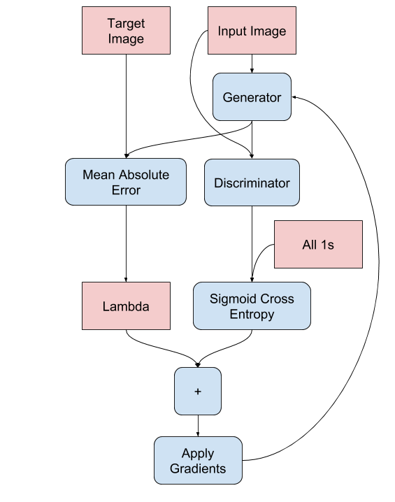
Define the generator loss
GANs learn a loss that adapts to the data, while cGANs learn a structured loss that penalizes a possible structure that differs from the network output and the target image, as described in the pix2pix paper.
- The generator loss is a sigmoid cross-entropy loss of the generated images and an array of ones.
- The pix2pix paper also mentions the L1 loss, which is a MAE (mean absolute error) between the generated image and the target image.
- This allows the generated image to become structurally similar to the target image.
- The formula to calculate the total generator loss is
gan_loss + LAMBDA * l1_loss, whereLAMBDA = 100. This value was decided by the authors of the paper.
LAMBDA = 100
loss_object = tf.keras.losses.BinaryCrossentropy(from_logits=True)
def generator_loss(disc_generated_output, gen_output, target):
  gan_loss = loss_object(tf.ones_like(disc_generated_output), disc_generated_output)

  # Mean absolute error
  l1_loss = tf.reduce_mean(tf.abs(target - gen_output))

  total_gen_loss = gan_loss + (LAMBDA * l1_loss)

  return total_gen_loss, gan_loss, l1_loss
The training procedure for the generator is as follows:
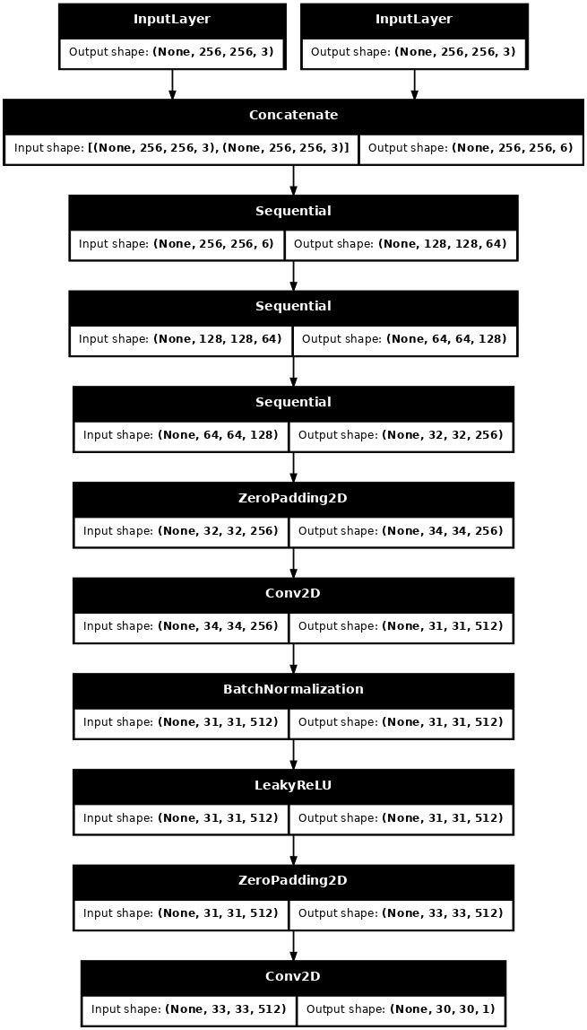
Build the discriminator
The discriminator in the pix2pix cGAN is a convolutional PatchGAN classifier—it tries to classify if each image patch is real or not real, as described in the pix2pix paper.
- Each block in the discriminator is: Convolution -> Batch normalization -> Leaky ReLU.
- The shape of the output after the last layer is
(batch_size, 30, 30, 1). - Each
30 x 30image patch of the output classifies a70 x 70portion of the input image. - The discriminator receives 2 inputs:
- The input image and the target image, which it should classify as real.
- The input image and the generated image (the output of the generator), which it should classify as fake.
- Use
tf.concat([inp, tar], axis=-1)to concatenate these 2 inputs together.
Let's define the discriminator:
def Discriminator():
  initializer = tf.random_normal_initializer(0., 0.02)

  inp = tf.keras.layers.Input(shape=[256, 256, 3], name='input_image')
  tar = tf.keras.layers.Input(shape=[256, 256, 3], name='target_image')

  x = tf.keras.layers.concatenate([inp, tar])  # (batch_size, 256, 256, channels*2)

  down1 = downsample(64, 4, False)(x)  # (batch_size, 128, 128, 64)
  down2 = downsample(128, 4)(down1)  # (batch_size, 64, 64, 128)
  down3 = downsample(256, 4)(down2)  # (batch_size, 32, 32, 256)

  zero_pad1 = tf.keras.layers.ZeroPadding2D()(down3)  # (batch_size, 34, 34, 256)
  conv = tf.keras.layers.Conv2D(512, 4, strides=1,
                                kernel_initializer=initializer,
                                use_bias=False)(zero_pad1)  # (batch_size, 31, 31, 512)

  batchnorm1 = tf.keras.layers.BatchNormalization()(conv)

  leaky_relu = tf.keras.layers.LeakyReLU()(batchnorm1)

  zero_pad2 = tf.keras.layers.ZeroPadding2D()(leaky_relu)  # (batch_size, 33, 33, 512)

  last = tf.keras.layers.Conv2D(1, 4, strides=1,
                                kernel_initializer=initializer)(zero_pad2)  # (batch_size, 30, 30, 1)

  return tf.keras.Model(inputs=[inp, tar], outputs=last)
Visualize the discriminator model architecture:
discriminator = Discriminator()
tf.keras.utils.plot_model(discriminator, show_shapes=True, dpi=64)
Test the discriminator:
disc_out = discriminator([inp[tf.newaxis, ...], gen_output], training=False)
plt.imshow(disc_out[0, ..., -1], vmin=-20, vmax=20, cmap='RdBu_r')
plt.colorbar()
W0000 00:00:1723785110.434536  166285 gpu_timer.cc:114] Skipping the delay kernel, measurement accuracy will be reduced
W0000 00:00:1723785110.435585  166285 gpu_timer.cc:114] Skipping the delay kernel, measurement accuracy will be reduced
W0000 00:00:1723785110.436290  166285 gpu_timer.cc:114] Skipping the delay kernel, measurement accuracy will be reduced
W0000 00:00:1723785110.436990  166285 gpu_timer.cc:114] Skipping the delay kernel, measurement accuracy will be reduced
W0000 00:00:1723785110.437686  166285 gpu_timer.cc:114] Skipping the delay kernel, measurement accuracy will be reduced
W0000 00:00:1723785110.438373  166285 gpu_timer.cc:114] Skipping the delay kernel, measurement accuracy will be reduced
W0000 00:00:1723785110.439061  166285 gpu_timer.cc:114] Skipping the delay kernel, measurement accuracy will be reduced
W0000 00:00:1723785110.439752  166285 gpu_timer.cc:114] Skipping the delay kernel, measurement accuracy will be reduced
W0000 00:00:1723785110.440504  166285 gpu_timer.cc:114] Skipping the delay kernel, measurement accuracy will be reduced
W0000 00:00:1723785110.441234  166285 gpu_timer.cc:114] Skipping the delay kernel, measurement accuracy will be reduced
W0000 00:00:1723785110.441943  166285 gpu_timer.cc:114] Skipping the delay kernel, measurement accuracy will be reduced
W0000 00:00:1723785110.442660  166285 gpu_timer.cc:114] Skipping the delay kernel, measurement accuracy will be reduced
W0000 00:00:1723785110.443433  166285 gpu_timer.cc:114] Skipping the delay kernel, measurement accuracy will be reduced
W0000 00:00:1723785110.475524  166285 gpu_timer.cc:114] Skipping the delay kernel, measurement accuracy will be reduced
W0000 00:00:1723785110.477639  166285 gpu_timer.cc:114] Skipping the delay kernel, measurement accuracy will be reduced
W0000 00:00:1723785110.479761  166285 gpu_timer.cc:114] Skipping the delay kernel, measurement accuracy will be reduced
W0000 00:00:1723785110.481978  166285 gpu_timer.cc:114] Skipping the delay kernel, measurement accuracy will be reduced
W0000 00:00:1723785110.483504  166285 gpu_timer.cc:114] Skipping the delay kernel, measurement accuracy will be reduced
W0000 00:00:1723785110.485135  166285 gpu_timer.cc:114] Skipping the delay kernel, measurement accuracy will be reduced
W0000 00:00:1723785110.486744  166285 gpu_timer.cc:114] Skipping the delay kernel, measurement accuracy will be reduced
W0000 00:00:1723785110.488353  166285 gpu_timer.cc:114] Skipping the delay kernel, measurement accuracy will be reduced
W0000 00:00:1723785110.489761  166285 gpu_timer.cc:114] Skipping the delay kernel, measurement accuracy will be reduced
W0000 00:00:1723785110.491115  166285 gpu_timer.cc:114] Skipping the delay kernel, measurement accuracy will be reduced
W0000 00:00:1723785110.492515  166285 gpu_timer.cc:114] Skipping the delay kernel, measurement accuracy will be reduced
W0000 00:00:1723785110.494043  166285 gpu_timer.cc:114] Skipping the delay kernel, measurement accuracy will be reduced
W0000 00:00:1723785110.495573  166285 gpu_timer.cc:114] Skipping the delay kernel, measurement accuracy will be reduced
W0000 00:00:1723785110.497450  166285 gpu_timer.cc:114] Skipping the delay kernel, measurement accuracy will be reduced
W0000 00:00:1723785110.498796  166285 gpu_timer.cc:114] Skipping the delay kernel, measurement accuracy will be reduced
W0000 00:00:1723785110.539785  166285 gpu_timer.cc:114] Skipping the delay kernel, measurement accuracy will be reduced
W0000 00:00:1723785110.562158  166285 gpu_timer.cc:114] Skipping the delay kernel, measurement accuracy will be reduced
W0000 00:00:1723785110.563402  166285 gpu_timer.cc:114] Skipping the delay kernel, measurement accuracy will be reduced
W0000 00:00:1723785110.564674  166285 gpu_timer.cc:114] Skipping the delay kernel, measurement accuracy will be reduced
W0000 00:00:1723785110.566227  166285 gpu_timer.cc:114] Skipping the delay kernel, measurement accuracy will be reduced
W0000 00:00:1723785110.568089  166285 gpu_timer.cc:114] Skipping the delay kernel, measurement accuracy will be reduced
W0000 00:00:1723785110.569930  166285 gpu_timer.cc:114] Skipping the delay kernel, measurement accuracy will be reduced
W0000 00:00:1723785110.571493  166285 gpu_timer.cc:114] Skipping the delay kernel, measurement accuracy will be reduced
W0000 00:00:1723785110.573074  166285 gpu_timer.cc:114] Skipping the delay kernel, measurement accuracy will be reduced
W0000 00:00:1723785110.574674  166285 gpu_timer.cc:114] Skipping the delay kernel, measurement accuracy will be reduced
W0000 00:00:1723785110.576501  166285 gpu_timer.cc:114] Skipping the delay kernel, measurement accuracy will be reduced
W0000 00:00:1723785110.578332  166285 gpu_timer.cc:114] Skipping the delay kernel, measurement accuracy will be reduced
W0000 00:00:1723785110.580045  166285 gpu_timer.cc:114] Skipping the delay kernel, measurement accuracy will be reduced
W0000 00:00:1723785110.581058  166285 gpu_timer.cc:114] Skipping the delay kernel, measurement accuracy will be reduced
<matplotlib.colorbar.Colorbar at 0x7f16f11c2eb0>

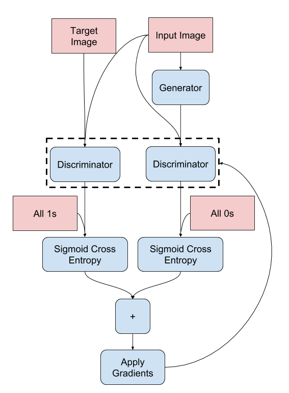
Define the discriminator loss
- The
discriminator_lossfunction takes 2 inputs: real images and generated images. real_lossis a sigmoid cross-entropy loss of the real images and an array of ones(since these are the real images).generated_lossis a sigmoid cross-entropy loss of the generated images and an array of zeros (since these are the fake images).- The
total_lossis the sum ofreal_lossandgenerated_loss.
def discriminator_loss(disc_real_output, disc_generated_output):
  real_loss = loss_object(tf.ones_like(disc_real_output), disc_real_output)

  generated_loss = loss_object(tf.zeros_like(disc_generated_output), disc_generated_output)

  total_disc_loss = real_loss + generated_loss

  return total_disc_loss
The training procedure for the discriminator is shown below.
To learn more about the architecture and the hyperparameters you can refer to the pix2pix paper.
Define the optimizers and a checkpoint-saver
generator_optimizer = tf.keras.optimizers.Adam(2e-4, beta_1=0.5)
discriminator_optimizer = tf.keras.optimizers.Adam(2e-4, beta_1=0.5)
checkpoint_dir = './training_checkpoints'
checkpoint_prefix = os.path.join(checkpoint_dir, "ckpt")
checkpoint = tf.train.Checkpoint(generator_optimizer=generator_optimizer,
                                 discriminator_optimizer=discriminator_optimizer,
                                 generator=generator,
                                 discriminator=discriminator)
Generate images
Write a function to plot some images during training.
- Pass images from the test set to the generator.
- The generator will then translate the input image into the output.
- The last step is to plot the predictions and voila!
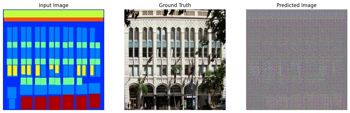
def generate_images(model, test_input, tar):
  prediction = model(test_input, training=True)
  plt.figure(figsize=(15, 15))

  display_list = [test_input[0], tar[0], prediction[0]]
  title = ['Input Image', 'Ground Truth', 'Predicted Image']

  for i in range(3):
    plt.subplot(1, 3, i+1)
    plt.title(title[i])
    # Getting the pixel values in the [0, 1] range to plot.
    plt.imshow(display_list[i] * 0.5 + 0.5)
    plt.axis('off')
  plt.show()
Test the function:
for example_input, example_target in test_dataset.take(1):
  generate_images(generator, example_input, example_target)
Training
- For each example input generates an output.
- The discriminator receives the
input_imageand the generated image as the first input. The second input is theinput_imageand thetarget_image. - Next, calculate the generator and the discriminator loss.
- Then, calculate the gradients of loss with respect to both the generator and the discriminator variables(inputs) and apply those to the optimizer.
- Finally, log the losses to TensorBoard.
log_dir="logs/"

summary_writer = tf.summary.create_file_writer(
  log_dir + "fit/" + datetime.datetime.now().strftime("%Y%m%d-%H%M%S"))
@tf.function
def train_step(input_image, target, step):
  with tf.GradientTape() as gen_tape, tf.GradientTape() as disc_tape:
    gen_output = generator(input_image, training=True)

    disc_real_output = discriminator([input_image, target], training=True)
    disc_generated_output = discriminator([input_image, gen_output], training=True)

    gen_total_loss, gen_gan_loss, gen_l1_loss = generator_loss(disc_generated_output, gen_output, target)
    disc_loss = discriminator_loss(disc_real_output, disc_generated_output)

  generator_gradients = gen_tape.gradient(gen_total_loss,
                                          generator.trainable_variables)
  discriminator_gradients = disc_tape.gradient(disc_loss,
                                               discriminator.trainable_variables)

  generator_optimizer.apply_gradients(zip(generator_gradients,
                                          generator.trainable_variables))
  discriminator_optimizer.apply_gradients(zip(discriminator_gradients,
                                              discriminator.trainable_variables))

  with summary_writer.as_default():
    tf.summary.scalar('gen_total_loss', gen_total_loss, step=step//1000)
    tf.summary.scalar('gen_gan_loss', gen_gan_loss, step=step//1000)
    tf.summary.scalar('gen_l1_loss', gen_l1_loss, step=step//1000)
    tf.summary.scalar('disc_loss', disc_loss, step=step//1000)
The actual training loop. Since this tutorial can run of more than one dataset, and the datasets vary greatly in size the training loop is setup to work in steps instead of epochs.
- Iterates over the number of steps.
- Every 10 steps print a dot (
.). - Every 1k steps: clear the display and run
generate_imagesto show the progress. - Every 5k steps: save a checkpoint.
def fit(train_ds, test_ds, steps):
  example_input, example_target = next(iter(test_ds.take(1)))
  start = time.time()

  for step, (input_image, target) in train_ds.repeat().take(steps).enumerate():
    if (step) % 1000 == 0:
      display.clear_output(wait=True)

      if step != 0:
        print(f'Time taken for 1000 steps: {time.time()-start:.2f} sec\n')

      start = time.time()

      generate_images(generator, example_input, example_target)
      print(f"Step: {step//1000}k")

    train_step(input_image, target, step)

    # Training step
    if (step+1) % 10 == 0:
      print('.', end='', flush=True)


    # Save (checkpoint) the model every 5k steps
    if (step + 1) % 5000 == 0:
      checkpoint.save(file_prefix=checkpoint_prefix)
This training loop saves logs that you can view in TensorBoard to monitor the training progress.
If you work on a local machine, you would launch a separate TensorBoard process. When working in a notebook, launch the viewer before starting the training to monitor with TensorBoard.
Launch the TensorBoard viewer (Sorry, this doesn't display on tensorflow.org):
%load_ext tensorboard
%tensorboard --logdir {log_dir}
You can view the results of a previous run of this notebook on TensorBoard.dev.
Finally, run the training loop:
fit(train_dataset, test_dataset, steps=40000)
Time taken for 1000 steps: 118.14 sec
Step: 39k
....................................................................................................
Interpreting the logs is more subtle when training a GAN (or a cGAN like pix2pix) compared to a simple classification or regression model. Things to look for:
- Check that neither the generator nor the discriminator model has "won". If either the
gen_gan_lossor thedisc_lossgets very low, it's an indicator that this model is dominating the other, and you are not successfully training the combined model. - The value
log(2) = 0.69is a good reference point for these losses, as it indicates a perplexity of 2 - the discriminator is, on average, equally uncertain about the two options. - For the
disc_loss, a value below0.69means the discriminator is doing better than random on the combined set of real and generated images. - For the
gen_gan_loss, a value below0.69means the generator is doing better than random at fooling the discriminator. - As training progresses, the
gen_l1_lossshould go down.
Restore the latest checkpoint and test the network
ls {checkpoint_dir}checkpoint ckpt-5.data-00000-of-00001 ckpt-1.data-00000-of-00001 ckpt-5.index ckpt-1.index ckpt-6.data-00000-of-00001 ckpt-2.data-00000-of-00001 ckpt-6.index ckpt-2.index ckpt-7.data-00000-of-00001 ckpt-3.data-00000-of-00001 ckpt-7.index ckpt-3.index ckpt-8.data-00000-of-00001 ckpt-4.data-00000-of-00001 ckpt-8.index ckpt-4.index
# Restoring the latest checkpoint in checkpoint_dir
checkpoint.restore(tf.train.latest_checkpoint(checkpoint_dir))
<tensorflow.python.checkpoint.checkpoint.CheckpointLoadStatus at 0x7f15f00fed90>
Generate some images using the test set
# Run the trained model on a few examples from the test set
for inp, tar in test_dataset.take(5):
  generate_images(generator, inp, tar)