
|
|
|
 View source on GitHub View source on GitHub
|
|
In machine learning, to improve something you often need to be able to measure it. TensorBoard is a tool for providing the measurements and visualizations needed during the machine learning workflow. It enables tracking experiment metrics like loss and accuracy, visualizing the model graph, projecting embeddings to a lower dimensional space, and much more.
This quickstart will show how to quickly get started with TensorBoard. The remaining guides in this website provide more details on specific capabilities, many of which are not included here.
# Load the TensorBoard notebook extension
%load_ext tensorboard
import tensorflow as tf
import datetime
# Clear any logs from previous runsrm -rf ./logs/
Using the MNIST dataset as the example, normalize the data and write a function that creates a simple Keras model for classifying the images into 10 classes.
mnist = tf.keras.datasets.mnist

(x_train, y_train),(x_test, y_test) = mnist.load_data()
x_train, x_test = x_train / 255.0, x_test / 255.0

def create_model():
  return tf.keras.models.Sequential([
    tf.keras.layers.Input(shape=(28, 28), name='layers_input'),
    tf.keras.layers.Flatten(name='layers_flatten'),
    tf.keras.layers.Dense(512, activation='relu', name='layers_dense'),
    tf.keras.layers.Dropout(0.2, name='layers_dropout'),
    tf.keras.layers.Dense(10, activation='softmax', name='layers_dense_2')
  ])
Downloading data from https://storage.googleapis.com/tensorflow/tf-keras-datasets/mnist.npz
11493376/11490434 [==============================] - 0s 0us/step
Using TensorBoard with Keras Model.fit()
When training with Keras's Model.fit(), adding the tf.keras.callbacks.TensorBoard callback ensures that logs are created and stored. Additionally, enable histogram computation every epoch with histogram_freq=1 (this is off by default)
Place the logs in a timestamped subdirectory to allow easy selection of different training runs.
model = create_model()
model.compile(optimizer='adam',
              loss='sparse_categorical_crossentropy',
              metrics=['accuracy'])

log_dir = "logs/fit/" + datetime.datetime.now().strftime("%Y%m%d-%H%M%S")
tensorboard_callback = tf.keras.callbacks.TensorBoard(log_dir=log_dir, histogram_freq=1)

model.fit(x=x_train,
          y=y_train,
          epochs=5,
          validation_data=(x_test, y_test),
          callbacks=[tensorboard_callback])
Train on 60000 samples, validate on 10000 samples
Epoch 1/5
60000/60000 [==============================] - 15s 246us/sample - loss: 0.2217 - accuracy: 0.9343 - val_loss: 0.1019 - val_accuracy: 0.9685
Epoch 2/5
60000/60000 [==============================] - 14s 229us/sample - loss: 0.0975 - accuracy: 0.9698 - val_loss: 0.0787 - val_accuracy: 0.9758
Epoch 3/5
60000/60000 [==============================] - 14s 231us/sample - loss: 0.0718 - accuracy: 0.9771 - val_loss: 0.0698 - val_accuracy: 0.9781
Epoch 4/5
60000/60000 [==============================] - 14s 227us/sample - loss: 0.0540 - accuracy: 0.9820 - val_loss: 0.0685 - val_accuracy: 0.9795
Epoch 5/5
60000/60000 [==============================] - 14s 228us/sample - loss: 0.0433 - accuracy: 0.9862 - val_loss: 0.0623 - val_accuracy: 0.9823
<tensorflow.python.keras.callbacks.History at 0x7fc8a5ee02e8>
Start TensorBoard through the command line or within a notebook experience. The two interfaces are generally the same. In notebooks, use the %tensorboard line magic. On the command line, run the same command without "%".
%tensorboard --logdir logs/fit
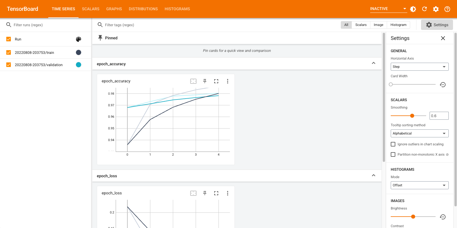
A brief overview of the visualizations created in this example and the dashboards (tabs in top navigation bar) where they can be found:
- Scalars show how the loss and metrics change with every epoch. You can use them to also track training speed, learning rate, and other scalar values. Scalars can be found in the Time Series or Scalars dashboards.
- Graphs help you visualize your model. In this case, the Keras graph of layers is shown which can help you ensure it is built correctly. Graphs can be found in the Graphs dashboard.
- Histograms and Distributions show the distribution of a Tensor over time. This can be useful to visualize weights and biases and verify that they are changing in an expected way. Histograms can be found in the Time Series or Histograms dashboards. Distributions can be found in the Distributions dashboard.
Additional TensorBoard dashboards are automatically enabled when you log other types of data. For example, the Keras TensorBoard callback lets you log images and embeddings as well. You can see what other dashboards are available in TensorBoard by clicking on the "inactive" dropdown towards the top right.
Using TensorBoard with other methods
When training with methods such as tf.GradientTape(), use tf.summary to log the required information.
Use the same dataset as above, but convert it to tf.data.Dataset to take advantage of batching capabilities:
train_dataset = tf.data.Dataset.from_tensor_slices((x_train, y_train))
test_dataset = tf.data.Dataset.from_tensor_slices((x_test, y_test))

train_dataset = train_dataset.shuffle(60000).batch(64)
test_dataset = test_dataset.batch(64)
The training code follows the advanced quickstart tutorial, but shows how to log metrics to TensorBoard. Choose loss and optimizer:
loss_object = tf.keras.losses.SparseCategoricalCrossentropy()
optimizer = tf.keras.optimizers.Adam()
Create stateful metrics that can be used to accumulate values during training and logged at any point:
# Define our metrics
train_loss = tf.keras.metrics.Mean('train_loss', dtype=tf.float32)
train_accuracy = tf.keras.metrics.SparseCategoricalAccuracy('train_accuracy')
test_loss = tf.keras.metrics.Mean('test_loss', dtype=tf.float32)
test_accuracy = tf.keras.metrics.SparseCategoricalAccuracy('test_accuracy')
Define the training and test functions:
def train_step(model, optimizer, x_train, y_train):
  with tf.GradientTape() as tape:
    predictions = model(x_train, training=True)
    loss = loss_object(y_train, predictions)
  grads = tape.gradient(loss, model.trainable_variables)
  optimizer.apply_gradients(zip(grads, model.trainable_variables))

  train_loss(loss)
  train_accuracy(y_train, predictions)

def test_step(model, x_test, y_test):
  predictions = model(x_test)
  loss = loss_object(y_test, predictions)

  test_loss(loss)
  test_accuracy(y_test, predictions)
Set up summary writers to write the summaries to disk in a different logs directory:
current_time = datetime.datetime.now().strftime("%Y%m%d-%H%M%S")
train_log_dir = 'logs/gradient_tape/' + current_time + '/train'
test_log_dir = 'logs/gradient_tape/' + current_time + '/test'
train_summary_writer = tf.summary.create_file_writer(train_log_dir)
test_summary_writer = tf.summary.create_file_writer(test_log_dir)
Start training. Use tf.summary.scalar() to log metrics (loss and accuracy) during training/testing within the scope of the summary writers to write the summaries to disk. You have control over which metrics to log and how often to do it. Other tf.summary functions enable logging other types of data.
model = create_model() # reset our model

EPOCHS = 5

for epoch in range(EPOCHS):
  for (x_train, y_train) in train_dataset:
    train_step(model, optimizer, x_train, y_train)
  with train_summary_writer.as_default():
    tf.summary.scalar('loss', train_loss.result(), step=epoch)
    tf.summary.scalar('accuracy', train_accuracy.result(), step=epoch)

  for (x_test, y_test) in test_dataset:
    test_step(model, x_test, y_test)
  with test_summary_writer.as_default():
    tf.summary.scalar('loss', test_loss.result(), step=epoch)
    tf.summary.scalar('accuracy', test_accuracy.result(), step=epoch)

  template = 'Epoch {}, Loss: {}, Accuracy: {}, Test Loss: {}, Test Accuracy: {}'
  print (template.format(epoch+1,
                         train_loss.result(),
                         train_accuracy.result()*100,
                         test_loss.result(),
                         test_accuracy.result()*100))

  # Reset metrics every epoch
  train_loss.reset_state()
  test_loss.reset_state()
  train_accuracy.reset_state()
  test_accuracy.reset_state()
Epoch 1, Loss: 0.24321186542510986, Accuracy: 92.84333801269531, Test Loss: 0.13006582856178284, Test Accuracy: 95.9000015258789
Epoch 2, Loss: 0.10446818172931671, Accuracy: 96.84833526611328, Test Loss: 0.08867532759904861, Test Accuracy: 97.1199951171875
Epoch 3, Loss: 0.07096975296735764, Accuracy: 97.80166625976562, Test Loss: 0.07875105738639832, Test Accuracy: 97.48999786376953
Epoch 4, Loss: 0.05380449816584587, Accuracy: 98.34166717529297, Test Loss: 0.07712937891483307, Test Accuracy: 97.56999969482422
Epoch 5, Loss: 0.041443776339292526, Accuracy: 98.71833038330078, Test Loss: 0.07514958828687668, Test Accuracy: 97.5
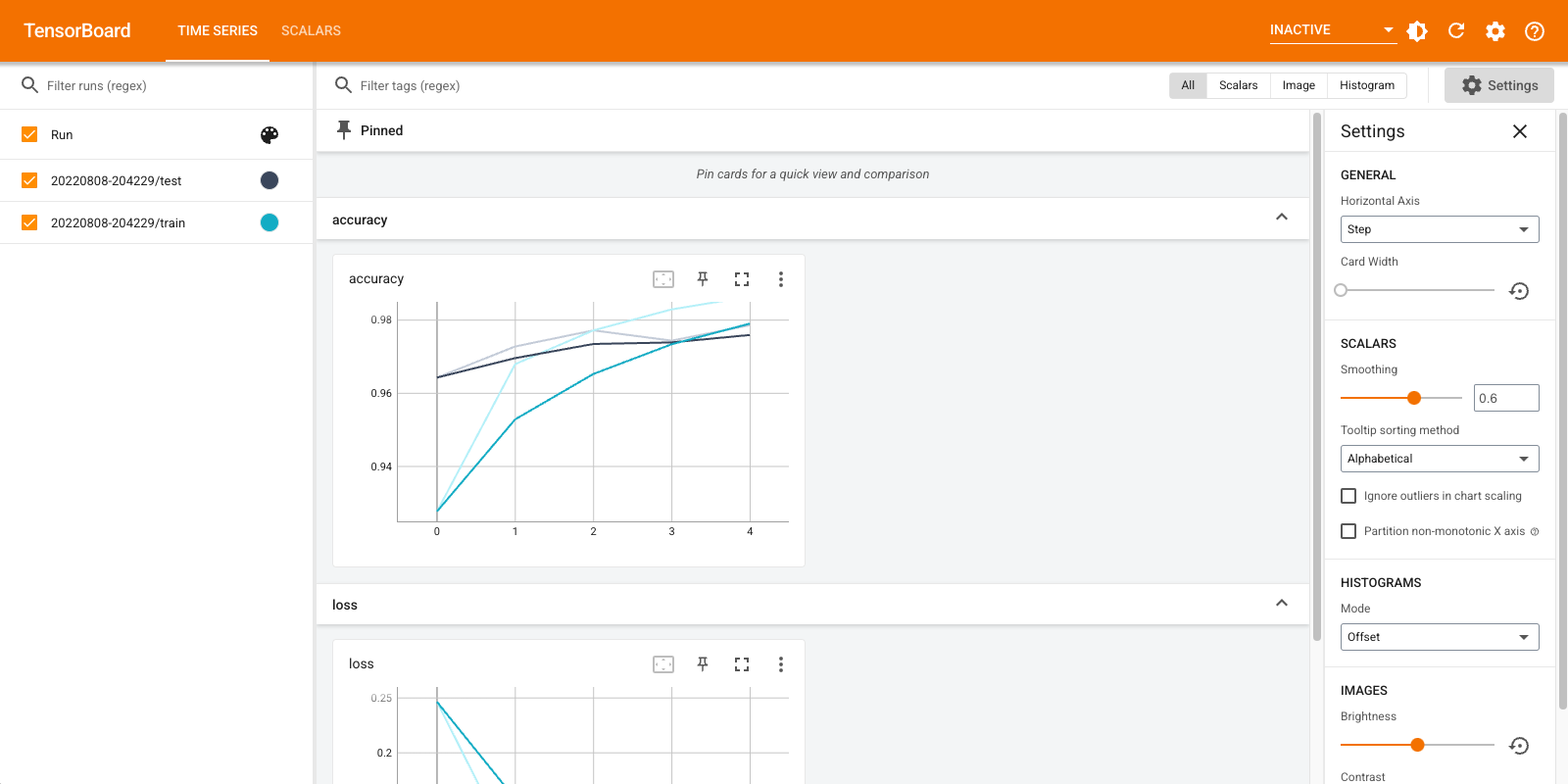
Open TensorBoard again, this time pointing it at the new log directory. We could have also started TensorBoard to monitor training while it progresses.
%tensorboard --logdir logs/gradient_tape
That's it! You have now seen how to use TensorBoard both through the Keras callback and through tf.summary for more custom scenarios.