টিএফ ল্যাটিস প্রিমেড মডেল

TensorFlow.org এ দেখুন

Google Colab-এ চালান

GitHub-এ উৎস দেখুন

নোটবুক ডাউনলোড করুন

ওভারভিউ

Premade মডেল দ্রুত এবং সহজ উপায়ে TfL গড়ে তুলতে হয় tf.keras.model টিপিক্যাল ব্যবহারের ক্ষেত্রে জন্য দৃষ্টান্ত। এই নির্দেশিকাটি একটি TFL প্রিমেড মডেল তৈরি করতে এবং এটিকে প্রশিক্ষণ/পরীক্ষা করার জন্য প্রয়োজনীয় পদক্ষেপগুলির রূপরেখা দেয়।

সেটআপ

টিএফ ল্যাটিস প্যাকেজ ইনস্টল করা হচ্ছে:

pip install tensorflow-lattice pydot

প্রয়োজনীয় প্যাকেজ আমদানি করা হচ্ছে:

import tensorflow as tf

import copy
import logging
import numpy as np
import pandas as pd
import sys
import tensorflow_lattice as tfl
logging.disable(sys.maxsize)

এই নির্দেশিকায় প্রশিক্ষণের জন্য ব্যবহৃত ডিফল্ট মান সেট করা:

LEARNING_RATE = 0.01
BATCH_SIZE = 128
NUM_EPOCHS = 500
PREFITTING_NUM_EPOCHS = 10

ইউসিআই স্ট্যাটলগ (হার্ট) ডেটাসেট ডাউনলোড করা হচ্ছে:

heart_csv_file = tf.keras.utils.get_file(
    'heart.csv',
    'http://storage.googleapis.com/download.tensorflow.org/data/heart.csv')
heart_df = pd.read_csv(heart_csv_file)
thal_vocab_list = ['normal', 'fixed', 'reversible']
heart_df['thal'] = heart_df['thal'].map(
    {v: i for i, v in enumerate(thal_vocab_list)})
heart_df = heart_df.astype(float)

heart_train_size = int(len(heart_df) * 0.8)
heart_train_dict = dict(heart_df[:heart_train_size])
heart_test_dict = dict(heart_df[heart_train_size:])

# This ordering of input features should match the feature configs. If no
# feature config relies explicitly on the data (i.e. all are 'quantiles'),
# then you can construct the feature_names list by simply iterating over each
# feature config and extracting it's name.
feature_names = [
    'age', 'sex', 'cp', 'chol', 'fbs', 'trestbps', 'thalach', 'restecg',
    'exang', 'oldpeak', 'slope', 'ca', 'thal'
]

# Since we have some features that manually construct their input keypoints,
# we need an index mapping of the feature names.
feature_name_indices = {name: index for index, name in enumerate(feature_names)}

label_name = 'target'
heart_train_xs = [
    heart_train_dict[feature_name] for feature_name in feature_names
]
heart_test_xs = [heart_test_dict[feature_name] for feature_name in feature_names]
heart_train_ys = heart_train_dict[label_name]
heart_test_ys = heart_test_dict[label_name]

Downloading data from http://storage.googleapis.com/download.tensorflow.org/data/heart.csv
16384/13273 [=====================================] - 0s 0us/step
24576/13273 [=======================================================] - 0s 0us/step

বৈশিষ্ট্য কনফিগার

বৈশিষ্ট্য ক্রমাঙ্কন এবং প্রতি-বৈশিষ্ট্য কনফিগারেশনের ব্যবহার নির্ধারণ করা হয় tfl.configs.FeatureConfig । বৈশিষ্ট্য কনফিগারেশনের monotonicity সীমাবদ্ধতা, প্রতি-বৈশিষ্ট্য নিয়মিতকরণ (দেখুন অন্তর্ভুক্ত tfl.configs.RegularizerConfig ), এবং জাফরি মডেলের জন্য জাফরি মাপ।

মনে রাখবেন যে আমরা আমাদের মডেল চিনতে চাই এমন যে কোনও বৈশিষ্ট্যের জন্য আমাদের অবশ্যই বৈশিষ্ট্য কনফিগার সম্পূর্ণরূপে নির্দিষ্ট করতে হবে। অন্যথায় মডেলটির জানার কোন উপায় থাকবে না যে এই ধরনের একটি বৈশিষ্ট্য বিদ্যমান।

আমাদের বৈশিষ্ট্য কনফিগার সংজ্ঞায়িত করা

এখন যেহেতু আমরা আমাদের কোয়ান্টাইলগুলি গণনা করতে পারি, আমরা প্রতিটি বৈশিষ্ট্যের জন্য একটি বৈশিষ্ট্য কনফিগার সংজ্ঞায়িত করি যা আমরা আমাদের মডেলটিকে ইনপুট হিসাবে নিতে চাই।

# Features:
# - age
# - sex
# - cp        chest pain type (4 values)
# - trestbps  resting blood pressure
# - chol      serum cholestoral in mg/dl
# - fbs       fasting blood sugar > 120 mg/dl
# - restecg   resting electrocardiographic results (values 0,1,2)
# - thalach   maximum heart rate achieved
# - exang     exercise induced angina
# - oldpeak   ST depression induced by exercise relative to rest
# - slope     the slope of the peak exercise ST segment
# - ca        number of major vessels (0-3) colored by flourosopy
# - thal      normal; fixed defect; reversable defect
#
# Feature configs are used to specify how each feature is calibrated and used.
heart_feature_configs = [
    tfl.configs.FeatureConfig(
        name='age',
        lattice_size=3,
        monotonicity='increasing',
        # We must set the keypoints manually.
        pwl_calibration_num_keypoints=5,
        pwl_calibration_input_keypoints='quantiles',
        pwl_calibration_clip_max=100,
        # Per feature regularization.
        regularizer_configs=[
            tfl.configs.RegularizerConfig(name='calib_wrinkle', l2=0.1),
        ],
    ),
    tfl.configs.FeatureConfig(
        name='sex',
        num_buckets=2,
    ),
    tfl.configs.FeatureConfig(
        name='cp',
        monotonicity='increasing',
        # Keypoints that are uniformly spaced.
        pwl_calibration_num_keypoints=4,
        pwl_calibration_input_keypoints=np.linspace(
            np.min(heart_train_xs[feature_name_indices['cp']]),
            np.max(heart_train_xs[feature_name_indices['cp']]),
            num=4),
    ),
    tfl.configs.FeatureConfig(
        name='chol',
        monotonicity='increasing',
        # Explicit input keypoints initialization.
        pwl_calibration_input_keypoints=[126.0, 210.0, 247.0, 286.0, 564.0],
        # Calibration can be forced to span the full output range by clamping.
        pwl_calibration_clamp_min=True,
        pwl_calibration_clamp_max=True,
        # Per feature regularization.
        regularizer_configs=[
            tfl.configs.RegularizerConfig(name='calib_hessian', l2=1e-4),
        ],
    ),
    tfl.configs.FeatureConfig(
        name='fbs',
        # Partial monotonicity: output(0) <= output(1)
        monotonicity=[(0, 1)],
        num_buckets=2,
    ),
    tfl.configs.FeatureConfig(
        name='trestbps',
        monotonicity='decreasing',
        pwl_calibration_num_keypoints=5,
        pwl_calibration_input_keypoints='quantiles',
    ),
    tfl.configs.FeatureConfig(
        name='thalach',
        monotonicity='decreasing',
        pwl_calibration_num_keypoints=5,
        pwl_calibration_input_keypoints='quantiles',
    ),
    tfl.configs.FeatureConfig(
        name='restecg',
        # Partial monotonicity: output(0) <= output(1), output(0) <= output(2)
        monotonicity=[(0, 1), (0, 2)],
        num_buckets=3,
    ),
    tfl.configs.FeatureConfig(
        name='exang',
        # Partial monotonicity: output(0) <= output(1)
        monotonicity=[(0, 1)],
        num_buckets=2,
    ),
    tfl.configs.FeatureConfig(
        name='oldpeak',
        monotonicity='increasing',
        pwl_calibration_num_keypoints=5,
        pwl_calibration_input_keypoints='quantiles',
    ),
    tfl.configs.FeatureConfig(
        name='slope',
        # Partial monotonicity: output(0) <= output(1), output(1) <= output(2)
        monotonicity=[(0, 1), (1, 2)],
        num_buckets=3,
    ),
    tfl.configs.FeatureConfig(
        name='ca',
        monotonicity='increasing',
        pwl_calibration_num_keypoints=4,
        pwl_calibration_input_keypoints='quantiles',
    ),
    tfl.configs.FeatureConfig(
        name='thal',
        # Partial monotonicity:
        # output(normal) <= output(fixed)
        # output(normal) <= output(reversible)
        monotonicity=[('normal', 'fixed'), ('normal', 'reversible')],
        num_buckets=3,
        # We must specify the vocabulary list in order to later set the
        # monotonicities since we used names and not indices.
        vocabulary_list=thal_vocab_list,
    ),
]

একঘেয়েমি এবং কীপয়েন্ট সেট করুন

এরপরে আমাদের নিশ্চিত করতে হবে যে বৈশিষ্ট্যগুলির জন্য একঘেয়েমিগুলি সঠিকভাবে সেট করা হয়েছে যেখানে আমরা একটি কাস্টম শব্দভান্ডার ব্যবহার করেছি (যেমন উপরে 'থল')।

tfl.premade_lib.set_categorical_monotonicities(heart_feature_configs)

অবশেষে আমরা কীপয়েন্টগুলি গণনা এবং সেট করে আমাদের বৈশিষ্ট্য কনফিগারগুলি সম্পূর্ণ করতে পারি।

feature_keypoints = tfl.premade_lib.compute_feature_keypoints(
    feature_configs=heart_feature_configs, features=heart_train_dict)
tfl.premade_lib.set_feature_keypoints(
    feature_configs=heart_feature_configs,
    feature_keypoints=feature_keypoints,
    add_missing_feature_configs=False)

ক্যালিব্রেটেড লিনিয়ার মডেল

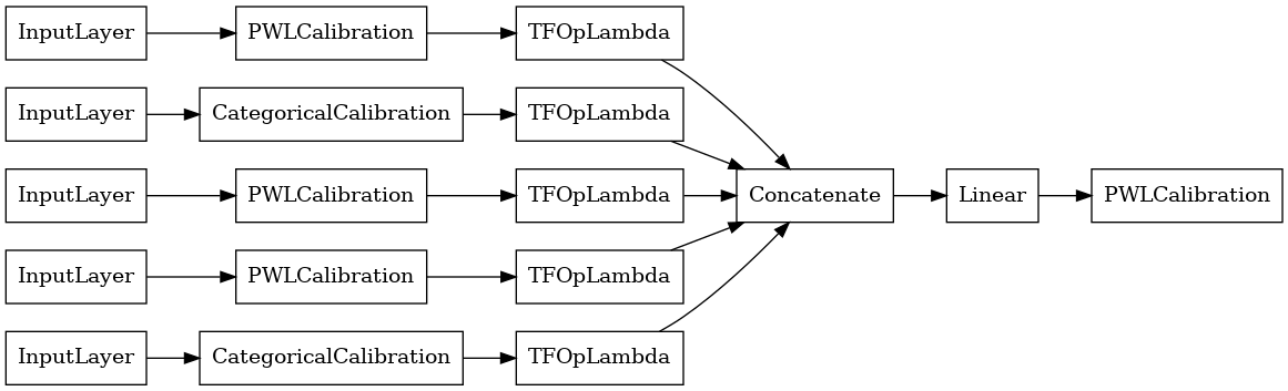
একটি TfL premade প্রতিরূপ গঠন করে, প্রথম থেকে একটি মডেল কনফিগারেশন গঠন করা tfl.configs । একটি মডেলটির ক্রমাঙ্ক রৈখিক মডেল ব্যবহার করে নির্মিত হয় tfl.configs.CalibratedLinearConfig । এটি ইনপুট বৈশিষ্ট্যগুলিতে টুকরো টুকরো-রৈখিক এবং শ্রেণীবদ্ধ ক্রমাঙ্কন প্রয়োগ করে, একটি রৈখিক সংমিশ্রণ এবং একটি ঐচ্ছিক আউটপুট পিসওয়াইজ-লিনিয়ার ক্রমাঙ্কন দ্বারা অনুসরণ করে। আউটপুট ক্রমাঙ্কন ব্যবহার করার সময় বা যখন আউটপুট সীমা নির্দিষ্ট করা হয়, রৈখিক স্তরটি ক্রমাঙ্কিত ইনপুটগুলিতে ওজনযুক্ত গড় প্রয়োগ করবে।

এই উদাহরণটি প্রথম 5টি বৈশিষ্ট্যের উপর একটি ক্যালিব্রেটেড লিনিয়ার মডেল তৈরি করে।

# Model config defines the model structure for the premade model.
linear_model_config = tfl.configs.CalibratedLinearConfig(
    feature_configs=heart_feature_configs[:5],
    use_bias=True,
    output_calibration=True,
    output_calibration_num_keypoints=10,
    # We initialize the output to [-2.0, 2.0] since we'll be using logits.
    output_initialization=np.linspace(-2.0, 2.0, num=10),
    regularizer_configs=[
        # Regularizer for the output calibrator.
        tfl.configs.RegularizerConfig(name='output_calib_hessian', l2=1e-4),
    ])
# A CalibratedLinear premade model constructed from the given model config.
linear_model = tfl.premade.CalibratedLinear(linear_model_config)
# Let's plot our model.
tf.keras.utils.plot_model(linear_model, show_layer_names=False, rankdir='LR')

2022-01-14 12:36:31.295751: E tensorflow/stream_executor/cuda/cuda_driver.cc:271] failed call to cuInit: CUDA_ERROR_NO_DEVICE: no CUDA-capable device is detected

এখন, অন্য কোন মত tf.keras.Model , আমরা এবং কম্পাইল আমাদের তথ্য মডেল মাপসই করা হবে।

linear_model.compile(
    loss=tf.keras.losses.BinaryCrossentropy(from_logits=True),
    metrics=[tf.keras.metrics.AUC(from_logits=True)],
    optimizer=tf.keras.optimizers.Adam(LEARNING_RATE))
linear_model.fit(
    heart_train_xs[:5],
    heart_train_ys,
    epochs=NUM_EPOCHS,
    batch_size=BATCH_SIZE,
    verbose=False)

<keras.callbacks.History at 0x7fe4385f0290>

আমাদের মডেল প্রশিক্ষণের পর, আমরা আমাদের পরীক্ষার সেটে এটি মূল্যায়ন করতে পারি।

print('Test Set Evaluation...')
print(linear_model.evaluate(heart_test_xs[:5], heart_test_ys))

Test Set Evaluation...
2/2 [==============================] - 0s 3ms/step - loss: 0.4728 - auc: 0.8252
[0.47278329730033875, 0.8251879215240479]

ক্যালিব্রেটেড ল্যাটিস মডেল

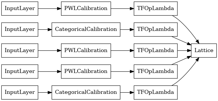
একটি মডেলটির ক্রমাঙ্ক জাফরি মডেল ব্যবহার করে নির্মিত হয় tfl.configs.CalibratedLatticeConfig । একটি ক্যালিব্রেটেড জালি মডেল ইনপুট বৈশিষ্ট্যগুলিতে টুকরো টুকরো-রৈখিক এবং শ্রেণীবদ্ধ ক্রমাঙ্কন প্রয়োগ করে, তারপরে একটি জালি মডেল এবং একটি ঐচ্ছিক আউটপুট পিসওয়াইজ-লিনিয়ার ক্রমাঙ্কন।

এই উদাহরণটি প্রথম 5টি বৈশিষ্ট্যের উপর একটি ক্যালিব্রেটেড জালি মডেল তৈরি করে।

# This is a calibrated lattice model: inputs are calibrated, then combined
# non-linearly using a lattice layer.
lattice_model_config = tfl.configs.CalibratedLatticeConfig(
    feature_configs=heart_feature_configs[:5],
    # We initialize the output to [-2.0, 2.0] since we'll be using logits.
    output_initialization=[-2.0, 2.0],
    regularizer_configs=[
        # Torsion regularizer applied to the lattice to make it more linear.
        tfl.configs.RegularizerConfig(name='torsion', l2=1e-2),
        # Globally defined calibration regularizer is applied to all features.
        tfl.configs.RegularizerConfig(name='calib_hessian', l2=1e-2),
    ])
# A CalibratedLattice premade model constructed from the given model config.
lattice_model = tfl.premade.CalibratedLattice(lattice_model_config)
# Let's plot our model.
tf.keras.utils.plot_model(lattice_model, show_layer_names=False, rankdir='LR')

আগের মত, আমরা আমাদের মডেল কম্পাইল, ফিট, এবং মূল্যায়ন.

lattice_model.compile(
    loss=tf.keras.losses.BinaryCrossentropy(from_logits=True),
    metrics=[tf.keras.metrics.AUC(from_logits=True)],
    optimizer=tf.keras.optimizers.Adam(LEARNING_RATE))
lattice_model.fit(
    heart_train_xs[:5],
    heart_train_ys,
    epochs=NUM_EPOCHS,
    batch_size=BATCH_SIZE,
    verbose=False)
print('Test Set Evaluation...')
print(lattice_model.evaluate(heart_test_xs[:5], heart_test_ys))

Test Set Evaluation...
2/2 [==============================] - 1s 3ms/step - loss: 0.4709 - auc_1: 0.8302
[0.4709009826183319, 0.8302004933357239]

ক্যালিব্রেটেড ল্যাটিস এনসেম্বল মডেল

বৈশিষ্ট্যের সংখ্যা বড় হলে, আপনি একটি ensemble মডেল ব্যবহার করতে পারেন, যা বৈশিষ্ট্যগুলির উপসেটের জন্য একাধিক ছোট জালি তৈরি করে এবং শুধুমাত্র একটি বিশাল জালি তৈরি করার পরিবর্তে তাদের আউটপুট গড় করে। আঁসাঁব্ল জাফরি মডেল ব্যবহার করে নির্মিত হয় tfl.configs.CalibratedLatticeEnsembleConfig । একটি ক্যালিব্রেটেড ল্যাটিস এনসেম্বল মডেল ইনপুট বৈশিষ্ট্যে টুকরো টুকরো-রৈখিক এবং শ্রেণীবদ্ধ ক্রমাঙ্কন প্রয়োগ করে, তারপরে জালি মডেলগুলির একটি অংশ এবং একটি ঐচ্ছিক আউটপুট পিসওয়াইজ-লিনিয়ার ক্রমাঙ্কন প্রয়োগ করে।

স্পষ্ট ল্যাটিস এনসেম্বল ইনিশিয়ালাইজেশন

আপনি যদি ইতিমধ্যেই জানেন যে বৈশিষ্ট্যগুলির কোন উপসেটগুলি আপনি আপনার জালিতে ফিড করতে চান, তাহলে আপনি বৈশিষ্ট্যের নাম ব্যবহার করে স্পষ্টভাবে জালিগুলি সেট করতে পারেন। এই উদাহরণটি প্রতি জালিতে 5টি জালি এবং 3টি বৈশিষ্ট্য সহ একটি ক্যালিব্রেটেড জালি এনসেম্বল মডেল তৈরি করে।

# This is a calibrated lattice ensemble model: inputs are calibrated, then
# combined non-linearly and averaged using multiple lattice layers.
explicit_ensemble_model_config = tfl.configs.CalibratedLatticeEnsembleConfig(
    feature_configs=heart_feature_configs,
    lattices=[['trestbps', 'chol', 'ca'], ['fbs', 'restecg', 'thal'],
              ['fbs', 'cp', 'oldpeak'], ['exang', 'slope', 'thalach'],
              ['restecg', 'age', 'sex']],
    num_lattices=5,
    lattice_rank=3,
    # We initialize the output to [-2.0, 2.0] since we'll be using logits.
    output_initialization=[-2.0, 2.0])
# A CalibratedLatticeEnsemble premade model constructed from the given
# model config.
explicit_ensemble_model = tfl.premade.CalibratedLatticeEnsemble(
    explicit_ensemble_model_config)
# Let's plot our model.
tf.keras.utils.plot_model(
    explicit_ensemble_model, show_layer_names=False, rankdir='LR')

আগের মত, আমরা আমাদের মডেল কম্পাইল, ফিট, এবং মূল্যায়ন.

explicit_ensemble_model.compile(
    loss=tf.keras.losses.BinaryCrossentropy(from_logits=True),
    metrics=[tf.keras.metrics.AUC(from_logits=True)],
    optimizer=tf.keras.optimizers.Adam(LEARNING_RATE))
explicit_ensemble_model.fit(
    heart_train_xs,
    heart_train_ys,
    epochs=NUM_EPOCHS,
    batch_size=BATCH_SIZE,
    verbose=False)
print('Test Set Evaluation...')
print(explicit_ensemble_model.evaluate(heart_test_xs, heart_test_ys))

Test Set Evaluation...
2/2 [==============================] - 1s 4ms/step - loss: 0.3768 - auc_2: 0.8954
[0.3768467903137207, 0.895363450050354]

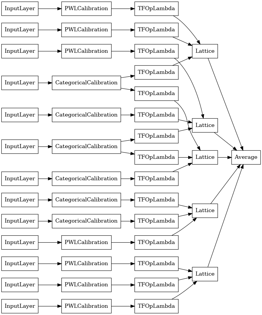
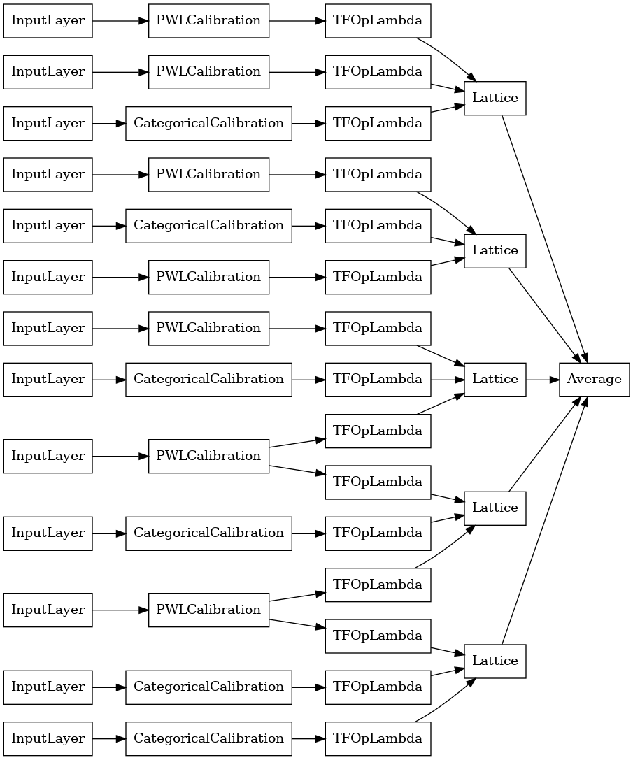
এলোমেলো ল্যাটিস এনসেম্বল

আপনি যদি নিশ্চিত না হন যে কোন বৈশিষ্ট্যগুলির উপসেটগুলি আপনার জালিতে ফিড করা হবে, অন্য একটি বিকল্প হল প্রতিটি জালির জন্য বৈশিষ্ট্যগুলির এলোমেলো উপসেটগুলি ব্যবহার করা৷ এই উদাহরণটি প্রতি জালিতে 5টি জালি এবং 3টি বৈশিষ্ট্য সহ একটি ক্যালিব্রেটেড জালি এনসেম্বল মডেল তৈরি করে।

# This is a calibrated lattice ensemble model: inputs are calibrated, then
# combined non-linearly and averaged using multiple lattice layers.
random_ensemble_model_config = tfl.configs.CalibratedLatticeEnsembleConfig(
    feature_configs=heart_feature_configs,
    lattices='random',
    num_lattices=5,
    lattice_rank=3,
    # We initialize the output to [-2.0, 2.0] since we'll be using logits.
    output_initialization=[-2.0, 2.0],
    random_seed=42)
# Now we must set the random lattice structure and construct the model.
tfl.premade_lib.set_random_lattice_ensemble(random_ensemble_model_config)
# A CalibratedLatticeEnsemble premade model constructed from the given
# model config.
random_ensemble_model = tfl.premade.CalibratedLatticeEnsemble(
    random_ensemble_model_config)
# Let's plot our model.
tf.keras.utils.plot_model(
    random_ensemble_model, show_layer_names=False, rankdir='LR')

আগের মত, আমরা আমাদের মডেল কম্পাইল, ফিট, এবং মূল্যায়ন.

random_ensemble_model.compile(
    loss=tf.keras.losses.BinaryCrossentropy(from_logits=True),
    metrics=[tf.keras.metrics.AUC(from_logits=True)],
    optimizer=tf.keras.optimizers.Adam(LEARNING_RATE))
random_ensemble_model.fit(
    heart_train_xs,
    heart_train_ys,
    epochs=NUM_EPOCHS,
    batch_size=BATCH_SIZE,
    verbose=False)
print('Test Set Evaluation...')
print(random_ensemble_model.evaluate(heart_test_xs, heart_test_ys))

Test Set Evaluation...
2/2 [==============================] - 1s 4ms/step - loss: 0.3739 - auc_3: 0.8997
[0.3739270567893982, 0.8997493982315063]

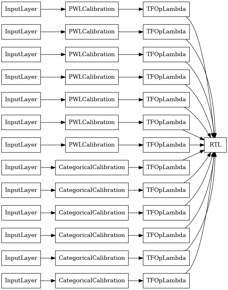
RTL লেয়ার র‍্যান্ডম ল্যাটিস এনসেম্বল

একটি র্যান্ডম জাফরি পাঁচমিশেলি ব্যবহার করার সময়, আপনার নির্দিষ্ট করা করতে পারে মডেল একটি একক ব্যবহার tfl.layers.RTL স্তর। আমরা লক্ষ করুন যে, tfl.layers.RTL শুধুমাত্র monotonicity সীমাবদ্ধতার সমর্থন করে এবং সমস্ত বৈশিষ্ট্য জন্য একই জাফরি আকার এবং কোন প্রতি-বৈশিষ্ট্য নিয়মিতকরণ থাকতে হবে। লক্ষ্য করুন, একটি ব্যবহার করে tfl.layers.RTL স্তর আপনি পৃথক ব্যবহার চেয়ে অনেক বড় ensembles আকার পরিবর্তন করতে দেয় tfl.layers.Lattice দৃষ্টান্ত।

এই উদাহরণটি প্রতি জালিতে 5টি জালি এবং 3টি বৈশিষ্ট্য সহ একটি ক্যালিব্রেটেড জালি এনসেম্বল মডেল তৈরি করে।

# Make sure our feature configs have the same lattice size, no per-feature
# regularization, and only monotonicity constraints.
rtl_layer_feature_configs = copy.deepcopy(heart_feature_configs)
for feature_config in rtl_layer_feature_configs:
  feature_config.lattice_size = 2
  feature_config.unimodality = 'none'
  feature_config.reflects_trust_in = None
  feature_config.dominates = None
  feature_config.regularizer_configs = None
# This is a calibrated lattice ensemble model: inputs are calibrated, then
# combined non-linearly and averaged using multiple lattice layers.
rtl_layer_ensemble_model_config = tfl.configs.CalibratedLatticeEnsembleConfig(
    feature_configs=rtl_layer_feature_configs,
    lattices='rtl_layer',
    num_lattices=5,
    lattice_rank=3,
    # We initialize the output to [-2.0, 2.0] since we'll be using logits.
    output_initialization=[-2.0, 2.0],
    random_seed=42)
# A CalibratedLatticeEnsemble premade model constructed from the given
# model config. Note that we do not have to specify the lattices by calling
# a helper function (like before with random) because the RTL Layer will take
# care of that for us.
rtl_layer_ensemble_model = tfl.premade.CalibratedLatticeEnsemble(
    rtl_layer_ensemble_model_config)
# Let's plot our model.
tf.keras.utils.plot_model(
    rtl_layer_ensemble_model, show_layer_names=False, rankdir='LR')

আগের মত, আমরা আমাদের মডেল কম্পাইল, ফিট, এবং মূল্যায়ন.

rtl_layer_ensemble_model.compile(
    loss=tf.keras.losses.BinaryCrossentropy(from_logits=True),
    metrics=[tf.keras.metrics.AUC(from_logits=True)],
    optimizer=tf.keras.optimizers.Adam(LEARNING_RATE))
rtl_layer_ensemble_model.fit(
    heart_train_xs,
    heart_train_ys,
    epochs=NUM_EPOCHS,
    batch_size=BATCH_SIZE,
    verbose=False)
print('Test Set Evaluation...')
print(rtl_layer_ensemble_model.evaluate(heart_test_xs, heart_test_ys))

Test Set Evaluation...
2/2 [==============================] - 0s 3ms/step - loss: 0.3614 - auc_4: 0.9079
[0.36142951250076294, 0.9078947305679321]

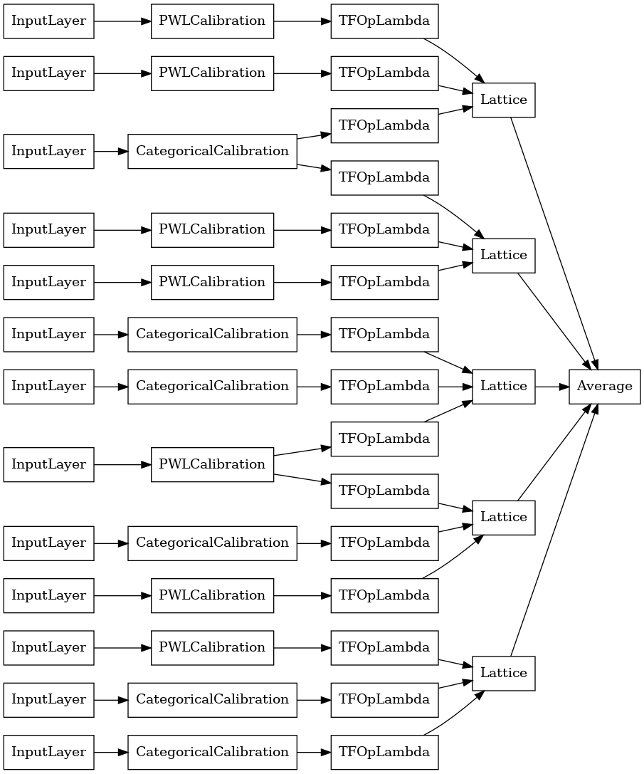
ক্রিস্টাল ল্যাটিস এনসেম্বল

Premade একটি অনুসন্ধানমূলক বৈশিষ্ট্য ব্যবস্থা অ্যালগরিদম নামক উপলব্ধ স্ফটিক । ক্রিস্টাল অ্যালগরিদম ব্যবহার করার জন্য, প্রথমে আমরা একটি প্রিফিটিং মডেলকে প্রশিক্ষিত করি যা জুটিভিত্তিক বৈশিষ্ট্য মিথস্ক্রিয়া অনুমান করে। তারপরে আমরা চূড়ান্ত সংযোজনটি এমনভাবে সাজাই যাতে আরও নন-লিনিয়ার মিথস্ক্রিয়া সহ বৈশিষ্ট্যগুলি একই জালিতে থাকে।

প্রিমেড লাইব্রেরি প্রিফিটিং মডেল কনফিগারেশন নির্মাণ এবং স্ফটিক কাঠামো নিষ্কাশনের জন্য সহায়ক ফাংশন অফার করে। মনে রাখবেন যে প্রিফিটিং মডেলটিকে সম্পূর্ণভাবে প্রশিক্ষিত করার প্রয়োজন নেই, তাই কয়েকটি যুগ যথেষ্ট হওয়া উচিত।

এই উদাহরণটি প্রতি জালিতে 5টি জালি এবং 3টি বৈশিষ্ট্য সহ একটি ক্যালিব্রেটেড জালির ensemble মডেল তৈরি করে৷

# This is a calibrated lattice ensemble model: inputs are calibrated, then
# combines non-linearly and averaged using multiple lattice layers.
crystals_ensemble_model_config = tfl.configs.CalibratedLatticeEnsembleConfig(
    feature_configs=heart_feature_configs,
    lattices='crystals',
    num_lattices=5,
    lattice_rank=3,
    # We initialize the output to [-2.0, 2.0] since we'll be using logits.
    output_initialization=[-2.0, 2.0],
    random_seed=42)
# Now that we have our model config, we can construct a prefitting model config.
prefitting_model_config = tfl.premade_lib.construct_prefitting_model_config(
    crystals_ensemble_model_config)
# A CalibratedLatticeEnsemble premade model constructed from the given
# prefitting model config.
prefitting_model = tfl.premade.CalibratedLatticeEnsemble(
    prefitting_model_config)
# We can compile and train our prefitting model as we like.
prefitting_model.compile(
    loss=tf.keras.losses.BinaryCrossentropy(from_logits=True),
    optimizer=tf.keras.optimizers.Adam(LEARNING_RATE))
prefitting_model.fit(
    heart_train_xs,
    heart_train_ys,
    epochs=PREFITTING_NUM_EPOCHS,
    batch_size=BATCH_SIZE,
    verbose=False)
# Now that we have our trained prefitting model, we can extract the crystals.
tfl.premade_lib.set_crystals_lattice_ensemble(crystals_ensemble_model_config,
                                              prefitting_model_config,
                                              prefitting_model)
# A CalibratedLatticeEnsemble premade model constructed from the given
# model config.
crystals_ensemble_model = tfl.premade.CalibratedLatticeEnsemble(
    crystals_ensemble_model_config)
# Let's plot our model.
tf.keras.utils.plot_model(
    crystals_ensemble_model, show_layer_names=False, rankdir='LR')

আগের মত, আমরা আমাদের মডেল কম্পাইল, ফিট, এবং মূল্যায়ন.

crystals_ensemble_model.compile(
    loss=tf.keras.losses.BinaryCrossentropy(from_logits=True),
    metrics=[tf.keras.metrics.AUC(from_logits=True)],
    optimizer=tf.keras.optimizers.Adam(LEARNING_RATE))
crystals_ensemble_model.fit(
    heart_train_xs,
    heart_train_ys,
    epochs=NUM_EPOCHS,
    batch_size=BATCH_SIZE,
    verbose=False)
print('Test Set Evaluation...')
print(crystals_ensemble_model.evaluate(heart_test_xs, heart_test_ys))

Test Set Evaluation...
2/2 [==============================] - 1s 3ms/step - loss: 0.3404 - auc_5: 0.9179
[0.34039050340652466, 0.9179198145866394]