
| | |  GitHub पर स्रोत देखें GitHub पर स्रोत देखें | |
अवलोकन
Premade मॉडल त्वरित और आसान तरीके टीएफएल निर्माण करने के लिए कर रहे हैं tf.keras.model ठेठ उपयोग के मामलों के लिए उदाहरणों। यह मार्गदर्शिका टीएफएल प्रेमाडे मॉडल के निर्माण और उसे प्रशिक्षित/परीक्षण करने के लिए आवश्यक कदमों की रूपरेखा तैयार करती है।
सेट अप
TF जाली पैकेज स्थापित करना:
pip install tensorflow-lattice pydot
आवश्यक पैकेज आयात करना:
import tensorflow as tf

import copy
import logging
import numpy as np
import pandas as pd
import sys
import tensorflow_lattice as tfl
logging.disable(sys.maxsize)
इस गाइड में प्रशिक्षण के लिए उपयोग किए जाने वाले डिफ़ॉल्ट मान सेट करना:
LEARNING_RATE = 0.01
BATCH_SIZE = 128
NUM_EPOCHS = 500
PREFITTING_NUM_EPOCHS = 10
UCI Statlog (हार्ट) डेटासेट डाउनलोड करना:
heart_csv_file = tf.keras.utils.get_file(
    'heart.csv',
    'http://storage.googleapis.com/download.tensorflow.org/data/heart.csv')
heart_df = pd.read_csv(heart_csv_file)
thal_vocab_list = ['normal', 'fixed', 'reversible']
heart_df['thal'] = heart_df['thal'].map(
    {v: i for i, v in enumerate(thal_vocab_list)})
heart_df = heart_df.astype(float)

heart_train_size = int(len(heart_df) * 0.8)
heart_train_dict = dict(heart_df[:heart_train_size])
heart_test_dict = dict(heart_df[heart_train_size:])

# This ordering of input features should match the feature configs. If no
# feature config relies explicitly on the data (i.e. all are 'quantiles'),
# then you can construct the feature_names list by simply iterating over each
# feature config and extracting it's name.
feature_names = [
    'age', 'sex', 'cp', 'chol', 'fbs', 'trestbps', 'thalach', 'restecg',
    'exang', 'oldpeak', 'slope', 'ca', 'thal'
]

# Since we have some features that manually construct their input keypoints,
# we need an index mapping of the feature names.
feature_name_indices = {name: index for index, name in enumerate(feature_names)}

label_name = 'target'
heart_train_xs = [
    heart_train_dict[feature_name] for feature_name in feature_names
]
heart_test_xs = [heart_test_dict[feature_name] for feature_name in feature_names]
heart_train_ys = heart_train_dict[label_name]
heart_test_ys = heart_test_dict[label_name]
Downloading data from http://storage.googleapis.com/download.tensorflow.org/data/heart.csv
16384/13273 [=====================================] - 0s 0us/step
24576/13273 [=======================================================] - 0s 0us/step
फ़ीचर कॉन्फिग
फ़ीचर अंशांकन और प्रति-सुविधा विन्यास का उपयोग कर स्थापित कर रहे हैं tfl.configs.FeatureConfig । फ़ीचर विन्यास दिष्टता बाधाओं, प्रति-सुविधा नियमितीकरण (देखें शामिल tfl.configs.RegularizerConfig ), और जाली मॉडल के लिए जाली आकार।
ध्यान दें कि हमें किसी भी सुविधा के लिए फीचर कॉन्फिग को पूरी तरह से निर्दिष्ट करना होगा जिसे हम अपने मॉडल को पहचानना चाहते हैं। अन्यथा मॉडल के पास यह जानने का कोई तरीका नहीं होगा कि ऐसी सुविधा मौजूद है।
हमारे फ़ीचर कॉन्फिग को परिभाषित करना
अब जब हम अपनी मात्राओं की गणना कर सकते हैं, तो हम प्रत्येक सुविधा के लिए एक फीचर कॉन्फिगरेशन को परिभाषित करते हैं जिसे हम चाहते हैं कि हमारा मॉडल इनपुट के रूप में ले।
# Features:
# - age
# - sex
# - cp        chest pain type (4 values)
# - trestbps  resting blood pressure
# - chol      serum cholestoral in mg/dl
# - fbs       fasting blood sugar > 120 mg/dl
# - restecg   resting electrocardiographic results (values 0,1,2)
# - thalach   maximum heart rate achieved
# - exang     exercise induced angina
# - oldpeak   ST depression induced by exercise relative to rest
# - slope     the slope of the peak exercise ST segment
# - ca        number of major vessels (0-3) colored by flourosopy
# - thal      normal; fixed defect; reversable defect
#
# Feature configs are used to specify how each feature is calibrated and used.
heart_feature_configs = [
    tfl.configs.FeatureConfig(
        name='age',
        lattice_size=3,
        monotonicity='increasing',
        # We must set the keypoints manually.
        pwl_calibration_num_keypoints=5,
        pwl_calibration_input_keypoints='quantiles',
        pwl_calibration_clip_max=100,
        # Per feature regularization.
        regularizer_configs=[
            tfl.configs.RegularizerConfig(name='calib_wrinkle', l2=0.1),
        ],
    ),
    tfl.configs.FeatureConfig(
        name='sex',
        num_buckets=2,
    ),
    tfl.configs.FeatureConfig(
        name='cp',
        monotonicity='increasing',
        # Keypoints that are uniformly spaced.
        pwl_calibration_num_keypoints=4,
        pwl_calibration_input_keypoints=np.linspace(
            np.min(heart_train_xs[feature_name_indices['cp']]),
            np.max(heart_train_xs[feature_name_indices['cp']]),
            num=4),
    ),
    tfl.configs.FeatureConfig(
        name='chol',
        monotonicity='increasing',
        # Explicit input keypoints initialization.
        pwl_calibration_input_keypoints=[126.0, 210.0, 247.0, 286.0, 564.0],
        # Calibration can be forced to span the full output range by clamping.
        pwl_calibration_clamp_min=True,
        pwl_calibration_clamp_max=True,
        # Per feature regularization.
        regularizer_configs=[
            tfl.configs.RegularizerConfig(name='calib_hessian', l2=1e-4),
        ],
    ),
    tfl.configs.FeatureConfig(
        name='fbs',
        # Partial monotonicity: output(0) <= output(1)
        monotonicity=[(0, 1)],
        num_buckets=2,
    ),
    tfl.configs.FeatureConfig(
        name='trestbps',
        monotonicity='decreasing',
        pwl_calibration_num_keypoints=5,
        pwl_calibration_input_keypoints='quantiles',
    ),
    tfl.configs.FeatureConfig(
        name='thalach',
        monotonicity='decreasing',
        pwl_calibration_num_keypoints=5,
        pwl_calibration_input_keypoints='quantiles',
    ),
    tfl.configs.FeatureConfig(
        name='restecg',
        # Partial monotonicity: output(0) <= output(1), output(0) <= output(2)
        monotonicity=[(0, 1), (0, 2)],
        num_buckets=3,
    ),
    tfl.configs.FeatureConfig(
        name='exang',
        # Partial monotonicity: output(0) <= output(1)
        monotonicity=[(0, 1)],
        num_buckets=2,
    ),
    tfl.configs.FeatureConfig(
        name='oldpeak',
        monotonicity='increasing',
        pwl_calibration_num_keypoints=5,
        pwl_calibration_input_keypoints='quantiles',
    ),
    tfl.configs.FeatureConfig(
        name='slope',
        # Partial monotonicity: output(0) <= output(1), output(1) <= output(2)
        monotonicity=[(0, 1), (1, 2)],
        num_buckets=3,
    ),
    tfl.configs.FeatureConfig(
        name='ca',
        monotonicity='increasing',
        pwl_calibration_num_keypoints=4,
        pwl_calibration_input_keypoints='quantiles',
    ),
    tfl.configs.FeatureConfig(
        name='thal',
        # Partial monotonicity:
        # output(normal) <= output(fixed)
        # output(normal) <= output(reversible)
        monotonicity=[('normal', 'fixed'), ('normal', 'reversible')],
        num_buckets=3,
        # We must specify the vocabulary list in order to later set the
        # monotonicities since we used names and not indices.
        vocabulary_list=thal_vocab_list,
    ),
]
एकरसता और मुख्य बिंदु सेट करें
इसके बाद हमें उन विशेषताओं के लिए एकरसता को ठीक से सेट करना सुनिश्चित करना होगा जहां हमने एक कस्टम शब्दावली (जैसे ऊपर 'थाल') का उपयोग किया था।
tfl.premade_lib.set_categorical_monotonicities(heart_feature_configs)
अंत में हम कीपॉइंट्स की गणना और सेट करके अपने फीचर कॉन्फिग को पूरा कर सकते हैं।
feature_keypoints = tfl.premade_lib.compute_feature_keypoints(
    feature_configs=heart_feature_configs, features=heart_train_dict)
tfl.premade_lib.set_feature_keypoints(
    feature_configs=heart_feature_configs,
    feature_keypoints=feature_keypoints,
    add_missing_feature_configs=False)
कैलिब्रेटेड रैखिक मॉडल
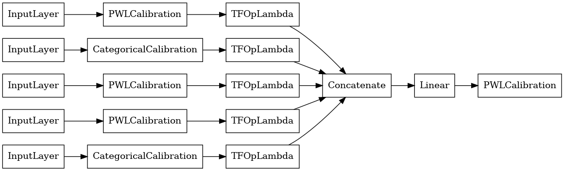
एक टीएफएल पूर्व बनाया मॉडल का निर्माण करने के लिए, पहले से एक मॉडल विन्यास का निर्माण tfl.configs । एक कैलिब्रेटेड रेखीय मॉडल का उपयोग कर निर्माण किया है tfl.configs.CalibratedLinearConfig । यह इनपुट सुविधाओं पर टुकड़े-टुकड़े-रैखिक और श्रेणीबद्ध अंशांकन लागू करता है, इसके बाद एक रैखिक संयोजन और एक वैकल्पिक आउटपुट टुकड़ा-रैखिक अंशांकन होता है। आउटपुट कैलिब्रेशन का उपयोग करते समय या जब आउटपुट सीमाएं निर्दिष्ट की जाती हैं, तो रैखिक परत कैलिब्रेटेड इनपुट पर भारित औसत लागू करेगी।
यह उदाहरण पहली 5 विशेषताओं पर एक कैलिब्रेटेड रैखिक मॉडल बनाता है।
# Model config defines the model structure for the premade model.
linear_model_config = tfl.configs.CalibratedLinearConfig(
    feature_configs=heart_feature_configs[:5],
    use_bias=True,
    output_calibration=True,
    output_calibration_num_keypoints=10,
    # We initialize the output to [-2.0, 2.0] since we'll be using logits.
    output_initialization=np.linspace(-2.0, 2.0, num=10),
    regularizer_configs=[
        # Regularizer for the output calibrator.
        tfl.configs.RegularizerConfig(name='output_calib_hessian', l2=1e-4),
    ])
# A CalibratedLinear premade model constructed from the given model config.
linear_model = tfl.premade.CalibratedLinear(linear_model_config)
# Let's plot our model.
tf.keras.utils.plot_model(linear_model, show_layer_names=False, rankdir='LR')
2022-01-14 12:36:31.295751: E tensorflow/stream_executor/cuda/cuda_driver.cc:271] failed call to cuInit: CUDA_ERROR_NO_DEVICE: no CUDA-capable device is detected
अब, किसी अन्य के साथ के रूप में tf.keras.Model , हम संकलन और हमारे डेटा मॉडल फिट।
linear_model.compile(
    loss=tf.keras.losses.BinaryCrossentropy(from_logits=True),
    metrics=[tf.keras.metrics.AUC(from_logits=True)],
    optimizer=tf.keras.optimizers.Adam(LEARNING_RATE))
linear_model.fit(
    heart_train_xs[:5],
    heart_train_ys,
    epochs=NUM_EPOCHS,
    batch_size=BATCH_SIZE,
    verbose=False)
<keras.callbacks.History at 0x7fe4385f0290>
अपने मॉडल को प्रशिक्षित करने के बाद, हम अपने परीक्षण सेट पर इसका मूल्यांकन कर सकते हैं।
print('Test Set Evaluation...')
print(linear_model.evaluate(heart_test_xs[:5], heart_test_ys))
Test Set Evaluation...
2/2 [==============================] - 0s 3ms/step - loss: 0.4728 - auc: 0.8252
[0.47278329730033875, 0.8251879215240479]
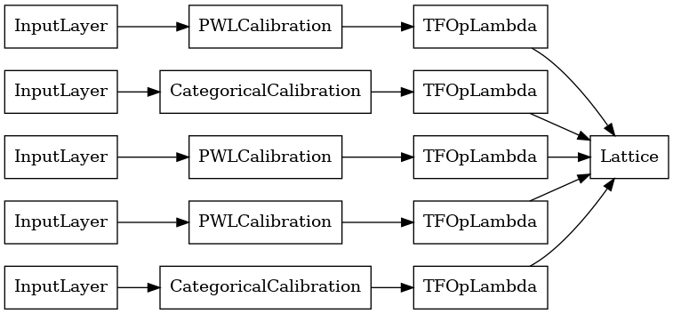
कैलिब्रेटेड जाली मॉडल
एक कैलिब्रेटेड जाली मॉडल का उपयोग कर निर्माण किया है tfl.configs.CalibratedLatticeConfig । एक कैलिब्रेटेड जाली मॉडल इनपुट सुविधाओं पर टुकड़े-टुकड़े-रैखिक और श्रेणीबद्ध अंशांकन लागू करता है, इसके बाद एक जाली मॉडल और एक वैकल्पिक आउटपुट टुकड़ा-रैखिक अंशांकन होता है।
यह उदाहरण पहली 5 विशेषताओं पर एक कैलिब्रेटेड जाली मॉडल बनाता है।
# This is a calibrated lattice model: inputs are calibrated, then combined
# non-linearly using a lattice layer.
lattice_model_config = tfl.configs.CalibratedLatticeConfig(
    feature_configs=heart_feature_configs[:5],
    # We initialize the output to [-2.0, 2.0] since we'll be using logits.
    output_initialization=[-2.0, 2.0],
    regularizer_configs=[
        # Torsion regularizer applied to the lattice to make it more linear.
        tfl.configs.RegularizerConfig(name='torsion', l2=1e-2),
        # Globally defined calibration regularizer is applied to all features.
        tfl.configs.RegularizerConfig(name='calib_hessian', l2=1e-2),
    ])
# A CalibratedLattice premade model constructed from the given model config.
lattice_model = tfl.premade.CalibratedLattice(lattice_model_config)
# Let's plot our model.
tf.keras.utils.plot_model(lattice_model, show_layer_names=False, rankdir='LR')
पहले की तरह, हम अपने मॉडल को संकलित, फिट और मूल्यांकन करते हैं।
lattice_model.compile(
    loss=tf.keras.losses.BinaryCrossentropy(from_logits=True),
    metrics=[tf.keras.metrics.AUC(from_logits=True)],
    optimizer=tf.keras.optimizers.Adam(LEARNING_RATE))
lattice_model.fit(
    heart_train_xs[:5],
    heart_train_ys,
    epochs=NUM_EPOCHS,
    batch_size=BATCH_SIZE,
    verbose=False)
print('Test Set Evaluation...')
print(lattice_model.evaluate(heart_test_xs[:5], heart_test_ys))
Test Set Evaluation...
2/2 [==============================] - 1s 3ms/step - loss: 0.4709 - auc_1: 0.8302
[0.4709009826183319, 0.8302004933357239]
कैलिब्रेटेड जाली पहनावा मॉडल
जब सुविधाओं की संख्या बड़ी होती है, तो आप एक पहनावा मॉडल का उपयोग कर सकते हैं, जो सुविधाओं के सबसेट के लिए कई छोटी जाली बनाता है और केवल एक विशाल जाली बनाने के बजाय उनके आउटपुट को औसत करता है। एनसेंबल जाली मॉडल का उपयोग कर निर्माण कर रहे हैं tfl.configs.CalibratedLatticeEnsembleConfig । एक कैलिब्रेटेड जालीदार पहनावा मॉडल इनपुट फीचर पर टुकड़े-टुकड़े-रैखिक और श्रेणीबद्ध अंशांकन लागू करता है, इसके बाद जाली मॉडल का एक समूह और एक वैकल्पिक आउटपुट टुकड़ा-रैखिक अंशांकन होता है।
स्पष्ट जाली कलाकारों की टुकड़ी आरंभीकरण
यदि आप पहले से ही जानते हैं कि सुविधाओं के कौन से सबसेट आप अपने जाली में फीड करना चाहते हैं, तो आप फीचर नामों का उपयोग करके स्पष्ट रूप से जाली सेट कर सकते हैं। यह उदाहरण 5 जाली और 3 सुविधाओं प्रति जाली के साथ एक कैलिब्रेटेड जाली पहनावा मॉडल बनाता है।
# This is a calibrated lattice ensemble model: inputs are calibrated, then
# combined non-linearly and averaged using multiple lattice layers.
explicit_ensemble_model_config = tfl.configs.CalibratedLatticeEnsembleConfig(
    feature_configs=heart_feature_configs,
    lattices=[['trestbps', 'chol', 'ca'], ['fbs', 'restecg', 'thal'],
              ['fbs', 'cp', 'oldpeak'], ['exang', 'slope', 'thalach'],
              ['restecg', 'age', 'sex']],
    num_lattices=5,
    lattice_rank=3,
    # We initialize the output to [-2.0, 2.0] since we'll be using logits.
    output_initialization=[-2.0, 2.0])
# A CalibratedLatticeEnsemble premade model constructed from the given
# model config.
explicit_ensemble_model = tfl.premade.CalibratedLatticeEnsemble(
    explicit_ensemble_model_config)
# Let's plot our model.
tf.keras.utils.plot_model(
    explicit_ensemble_model, show_layer_names=False, rankdir='LR')
पहले की तरह, हम अपने मॉडल को संकलित, फिट और मूल्यांकन करते हैं।
explicit_ensemble_model.compile(
    loss=tf.keras.losses.BinaryCrossentropy(from_logits=True),
    metrics=[tf.keras.metrics.AUC(from_logits=True)],
    optimizer=tf.keras.optimizers.Adam(LEARNING_RATE))
explicit_ensemble_model.fit(
    heart_train_xs,
    heart_train_ys,
    epochs=NUM_EPOCHS,
    batch_size=BATCH_SIZE,
    verbose=False)
print('Test Set Evaluation...')
print(explicit_ensemble_model.evaluate(heart_test_xs, heart_test_ys))
Test Set Evaluation...
2/2 [==============================] - 1s 4ms/step - loss: 0.3768 - auc_2: 0.8954
[0.3768467903137207, 0.895363450050354]
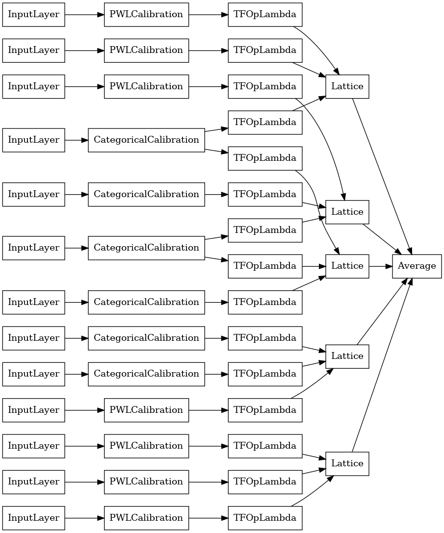
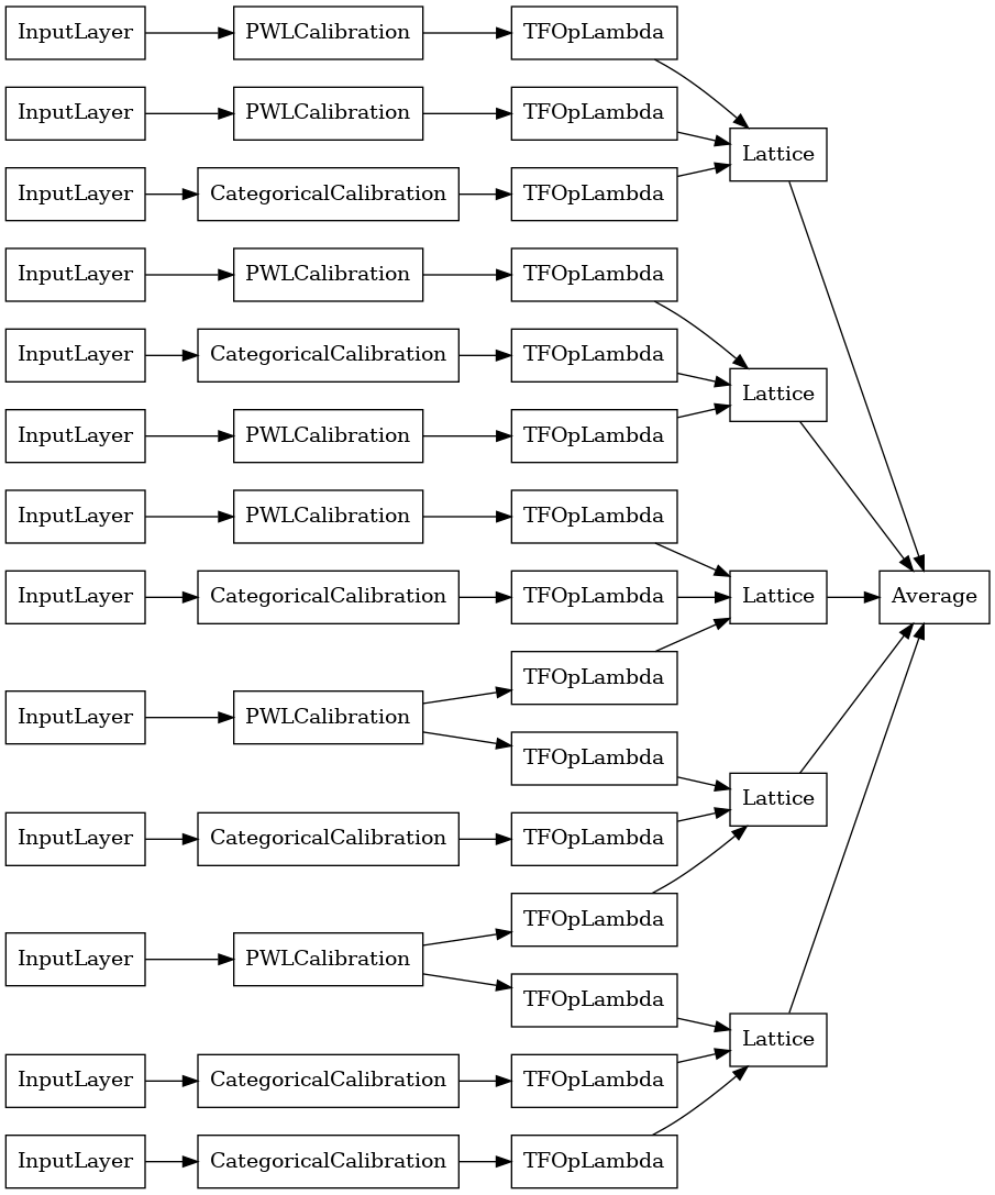
यादृच्छिक जाली कलाकारों की टुकड़ी
यदि आप सुनिश्चित नहीं हैं कि सुविधाओं के कौन से उपसमुच्चय आपके जाली में फीड होंगे, तो दूसरा विकल्प प्रत्येक जाली के लिए सुविधाओं के यादृच्छिक उपसमुच्चय का उपयोग करना है। यह उदाहरण 5 जाली और 3 सुविधाओं प्रति जाली के साथ एक कैलिब्रेटेड जाली पहनावा मॉडल बनाता है।
# This is a calibrated lattice ensemble model: inputs are calibrated, then
# combined non-linearly and averaged using multiple lattice layers.
random_ensemble_model_config = tfl.configs.CalibratedLatticeEnsembleConfig(
    feature_configs=heart_feature_configs,
    lattices='random',
    num_lattices=5,
    lattice_rank=3,
    # We initialize the output to [-2.0, 2.0] since we'll be using logits.
    output_initialization=[-2.0, 2.0],
    random_seed=42)
# Now we must set the random lattice structure and construct the model.
tfl.premade_lib.set_random_lattice_ensemble(random_ensemble_model_config)
# A CalibratedLatticeEnsemble premade model constructed from the given
# model config.
random_ensemble_model = tfl.premade.CalibratedLatticeEnsemble(
    random_ensemble_model_config)
# Let's plot our model.
tf.keras.utils.plot_model(
    random_ensemble_model, show_layer_names=False, rankdir='LR')
पहले की तरह, हम अपने मॉडल को संकलित, फिट और मूल्यांकन करते हैं।
random_ensemble_model.compile(
    loss=tf.keras.losses.BinaryCrossentropy(from_logits=True),
    metrics=[tf.keras.metrics.AUC(from_logits=True)],
    optimizer=tf.keras.optimizers.Adam(LEARNING_RATE))
random_ensemble_model.fit(
    heart_train_xs,
    heart_train_ys,
    epochs=NUM_EPOCHS,
    batch_size=BATCH_SIZE,
    verbose=False)
print('Test Set Evaluation...')
print(random_ensemble_model.evaluate(heart_test_xs, heart_test_ys))
Test Set Evaluation...
2/2 [==============================] - 1s 4ms/step - loss: 0.3739 - auc_3: 0.8997
[0.3739270567893982, 0.8997493982315063]
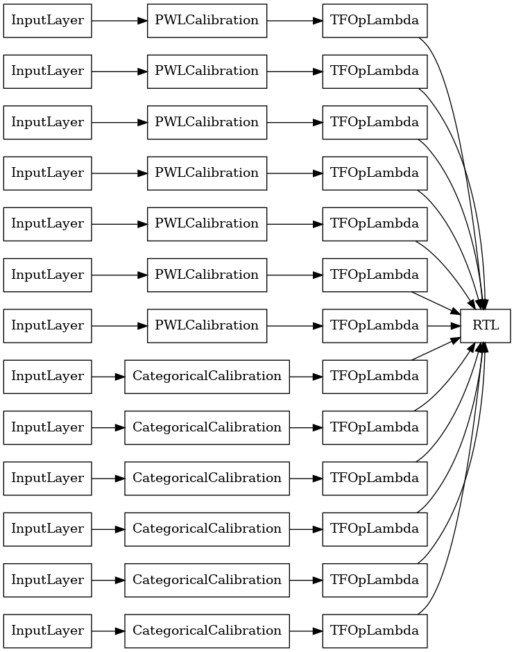
RTL परत रैंडम जालीदार पहनावा
एक यादृच्छिक जाली कलाकारों की टुकड़ी का उपयोग करते समय, आप निर्दिष्ट कर सकते हैं कि मॉडल एक भी का उपयोग tfl.layers.RTL परत। हम ध्यान दें कि tfl.layers.RTL केवल दिष्टता की कमी का समर्थन करता है और सभी सुविधाओं के लिए समान जाली आकार और कोई प्रति-सुविधा नियमितीकरण होना आवश्यक है। नोट एक का उपयोग कर कि tfl.layers.RTL परत आप अलग का उपयोग कर से भी ज्यादा बड़ा टुकड़ियों को स्केल की सुविधा देता है tfl.layers.Lattice उदाहरणों।
यह उदाहरण 5 जाली और 3 सुविधाओं प्रति जाली के साथ एक कैलिब्रेटेड जाली पहनावा मॉडल बनाता है।
# Make sure our feature configs have the same lattice size, no per-feature
# regularization, and only monotonicity constraints.
rtl_layer_feature_configs = copy.deepcopy(heart_feature_configs)
for feature_config in rtl_layer_feature_configs:
  feature_config.lattice_size = 2
  feature_config.unimodality = 'none'
  feature_config.reflects_trust_in = None
  feature_config.dominates = None
  feature_config.regularizer_configs = None
# This is a calibrated lattice ensemble model: inputs are calibrated, then
# combined non-linearly and averaged using multiple lattice layers.
rtl_layer_ensemble_model_config = tfl.configs.CalibratedLatticeEnsembleConfig(
    feature_configs=rtl_layer_feature_configs,
    lattices='rtl_layer',
    num_lattices=5,
    lattice_rank=3,
    # We initialize the output to [-2.0, 2.0] since we'll be using logits.
    output_initialization=[-2.0, 2.0],
    random_seed=42)
# A CalibratedLatticeEnsemble premade model constructed from the given
# model config. Note that we do not have to specify the lattices by calling
# a helper function (like before with random) because the RTL Layer will take
# care of that for us.
rtl_layer_ensemble_model = tfl.premade.CalibratedLatticeEnsemble(
    rtl_layer_ensemble_model_config)
# Let's plot our model.
tf.keras.utils.plot_model(
    rtl_layer_ensemble_model, show_layer_names=False, rankdir='LR')
पहले की तरह, हम अपने मॉडल को संकलित, फिट और मूल्यांकन करते हैं।
rtl_layer_ensemble_model.compile(
    loss=tf.keras.losses.BinaryCrossentropy(from_logits=True),
    metrics=[tf.keras.metrics.AUC(from_logits=True)],
    optimizer=tf.keras.optimizers.Adam(LEARNING_RATE))
rtl_layer_ensemble_model.fit(
    heart_train_xs,
    heart_train_ys,
    epochs=NUM_EPOCHS,
    batch_size=BATCH_SIZE,
    verbose=False)
print('Test Set Evaluation...')
print(rtl_layer_ensemble_model.evaluate(heart_test_xs, heart_test_ys))
Test Set Evaluation...
2/2 [==============================] - 0s 3ms/step - loss: 0.3614 - auc_4: 0.9079
[0.36142951250076294, 0.9078947305679321]
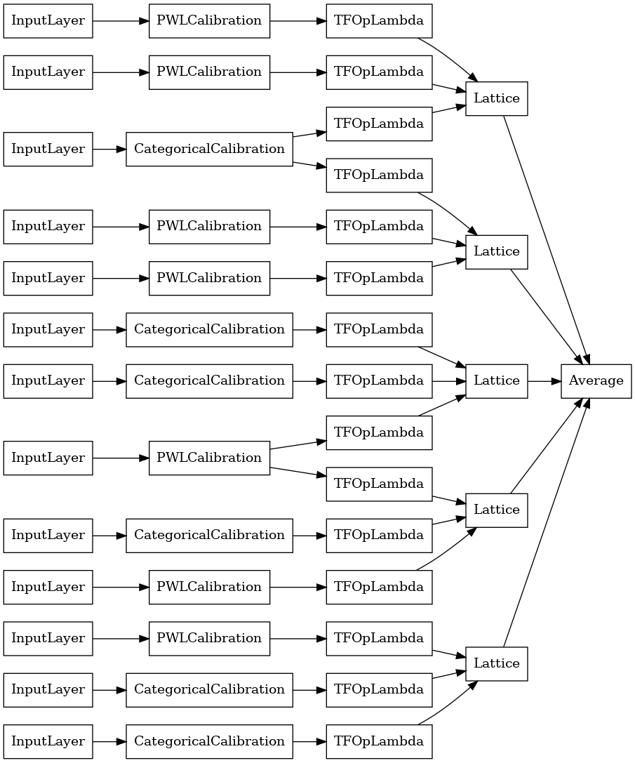
क्रिस्टल जाली पहनावा
Premade भी एक अनुमानी सुविधा व्यवस्था एल्गोरिथ्म, कहा जाता है प्रदान करता है कण । क्रिस्टल एल्गोरिथम का उपयोग करने के लिए, पहले हम एक प्रीफिटिंग मॉडल को प्रशिक्षित करते हैं जो जोड़ीदार फीचर इंटरैक्शन का अनुमान लगाता है। फिर हम अंतिम पहनावा की व्यवस्था करते हैं जैसे कि अधिक गैर-रैखिक इंटरैक्शन वाली विशेषताएं एक ही जाली में हों।
प्रेमाडे लाइब्रेरी प्रीफिटिंग मॉडल कॉन्फ़िगरेशन के निर्माण और क्रिस्टल संरचना को निकालने के लिए सहायक कार्य प्रदान करती है। ध्यान दें कि प्रीफिटिंग मॉडल को पूरी तरह से प्रशिक्षित होने की आवश्यकता नहीं है, इसलिए कुछ युग पर्याप्त होने चाहिए।
यह उदाहरण 5 जाली और 3 सुविधाओं प्रति जाली के साथ एक कैलिब्रेटेड जाली पहनावा मॉडल बनाता है।
# This is a calibrated lattice ensemble model: inputs are calibrated, then
# combines non-linearly and averaged using multiple lattice layers.
crystals_ensemble_model_config = tfl.configs.CalibratedLatticeEnsembleConfig(
    feature_configs=heart_feature_configs,
    lattices='crystals',
    num_lattices=5,
    lattice_rank=3,
    # We initialize the output to [-2.0, 2.0] since we'll be using logits.
    output_initialization=[-2.0, 2.0],
    random_seed=42)
# Now that we have our model config, we can construct a prefitting model config.
prefitting_model_config = tfl.premade_lib.construct_prefitting_model_config(
    crystals_ensemble_model_config)
# A CalibratedLatticeEnsemble premade model constructed from the given
# prefitting model config.
prefitting_model = tfl.premade.CalibratedLatticeEnsemble(
    prefitting_model_config)
# We can compile and train our prefitting model as we like.
prefitting_model.compile(
    loss=tf.keras.losses.BinaryCrossentropy(from_logits=True),
    optimizer=tf.keras.optimizers.Adam(LEARNING_RATE))
prefitting_model.fit(
    heart_train_xs,
    heart_train_ys,
    epochs=PREFITTING_NUM_EPOCHS,
    batch_size=BATCH_SIZE,
    verbose=False)
# Now that we have our trained prefitting model, we can extract the crystals.
tfl.premade_lib.set_crystals_lattice_ensemble(crystals_ensemble_model_config,
                                              prefitting_model_config,
                                              prefitting_model)
# A CalibratedLatticeEnsemble premade model constructed from the given
# model config.
crystals_ensemble_model = tfl.premade.CalibratedLatticeEnsemble(
    crystals_ensemble_model_config)
# Let's plot our model.
tf.keras.utils.plot_model(
    crystals_ensemble_model, show_layer_names=False, rankdir='LR')
पहले की तरह, हम अपने मॉडल को संकलित, फिट और मूल्यांकन करते हैं।
crystals_ensemble_model.compile(
    loss=tf.keras.losses.BinaryCrossentropy(from_logits=True),
    metrics=[tf.keras.metrics.AUC(from_logits=True)],
    optimizer=tf.keras.optimizers.Adam(LEARNING_RATE))
crystals_ensemble_model.fit(
    heart_train_xs,
    heart_train_ys,
    epochs=NUM_EPOCHS,
    batch_size=BATCH_SIZE,
    verbose=False)
print('Test Set Evaluation...')
print(crystals_ensemble_model.evaluate(heart_test_xs, heart_test_ys))
Test Set Evaluation...
2/2 [==============================] - 1s 3ms/step - loss: 0.3404 - auc_5: 0.9179
[0.34039050340652466, 0.9179198145866394]